1. Introduction
One of the solutions for improving the energy efficiency of water distribution networks (WDNs) is coupling pressure regulation and hydropower generation at sites with excess pressure [
1]. Despite the well-known disadvantages of Pump-As-Turbines (PATs) in comparison to the conventional hydraulic turbines, the vast majority of the literature highlight these for application in WDNs because of their significantly lower cost resulting from their mass production [
2]. This particularly pertains to the micro hydropower segment (below 100 kW), where the majority of sites from WDNs fit.
In PAT literature in general, most studies have investigated their performance and proposed models for their performance prediction [
3], as pump manufactures still do not provide the performance datasheets of their units in the turbine mode. For a single rotational speed, PAT performance is fully characterized when its resistance (Q-H) and power (Q-P) or efficiency (Q-η) curves in the complete range of operation are known. The simplest way to recreate these curves is using semi-empirical 1D models. Among 1D models, two categories are most represented: (1) models for the prediction of the best efficiency point (BEP) in turbine mode using pump mode data [
4] and (2) models for prediction (in some studies referred as extrapolation) of full performance curves from BEP in turbine mode [
5].
One of the most relevant disadvantages of PATs for their installation in WDNs, in comparison to conventional turbines, is that these do not possess flow control devices. Consequently, many studies address this problem by proposing different control schemes. Three most notable and recurring schemes in the literature are: (1) Hydraulic regulation (HR) [
6]; (2) Electric regulation [
7]; and (3) Coupled hydraulic and electrical regulation (HER) [
8]. HR scheme considers a PAT unit rotating at a fixed rotational speed to be installed in a series to a control valve and a bypass line equipped with another control valve. ER considers just one generation line and the addition of an inverter that would allow the PAT unit to change its rotational speed and thus somewhat adjust its head loss curve to the operating conditions (OCs). HER represents the superposition of the previous two schemes. The results of a recent study indicated that the HR scheme is the optimal tradeoff between the effectiveness of the energy recovery and the installation costs [
9].
Conceptually, the methodologies for PAT selection at predetermined locations could be classified in two groups, one when a PAT database is available [
9,
10] and other when it is not [
7,
11,
12]. The methodologies that do not include a PAT database propose strategies for defining the optimal design point (BEP) of a theoretical PAT that maximizes/minimizes a selected objective. Among these methodologies, two approaches could be distinguished. The studies that followed the first approach practically assumed that the optimal BEP matches the average operating condition (AOC) at the investigated site, without simulating the PAT performance to attest this assumption [
13]. On the other hand, the studies that followed the second approach simulated the performance of theoretical PATs whose BEPs are in proximity to the recorded operating conditions (OCs) where the optimal solution is the one that maximizes the chosen objective [
7,
11,
12].
The first approach is much simpler; however, is it valid? Namely, is it valid for a general case, regardless of the site’s size, level of variations of OCs, flow pattern type, type of pressure regulation, PAT control strategy, etc.? The main aim and novelty of this paper is to address this dilemma, which can be summed up in a question: Can the BEP of the optimal theoretical PAT be generalized, i.e., be defined as AOC (or its ratio) at the investigated site for a general case? In this paper, the question is addressed only considering the HR control strategy.
2. Methodology
2.1. Design of the Experiement
To address the above research question, the following experiment was conducted:
Compiling the PRV database. Studies proposing PAT selection methodologies usually demonstrate these on one or a few sites. To investigate the hypothesis in question in this paper, it is necessary to test it for all kinds of sites occurring in WDNs. For this purpose, a large database of measurements from 38 PRV sites from Dublin and Seville was compiled. Data on flow, upstream and downstream head were recorded for a period of around a year with frequency of 15 min and 5 min in the case of sites from Dublin and Seville, respectively.
Assessing AOCs at the PRV sites. The AOCs are represented by average operating flow () and average operating excess head (). The excess head is calculated by subtracting downstream from upstream head. The averages are calculated for the entire recorded periods, excluding periods of valves closure () or inactivity ().
Assessing the BEP of the optimal theoretical PAT. This is the most complex part of the analysis and is explained in detail in
Section 2.2.
Assessing the optimal relative BEP for each site. The optimal relative BEP (
;
) of the site
is the BEP of its optimal theoretical PAT assessed in the previous step normalized with its AOC. The coordinates of the optimal relative BEP for site
are assessed as:
where
[L/s] and
[m] are the BEP flow and head of the optimal theoretical PAT for site
, respectively, while
[L/s] and
[m] are the average operating flow and excess head at site
, respectively.
Assessing the generalized relative optimal BEP. The generalized optimal relative BEP (; ) is calculated as a simple average across the 38 optimal relative BEPs calculated in the previous step.
Assessing relative distances with the BEPs of PATs from the market. Two types of relative differences are calculated in this step. The first type are the distances between the PATs available on the market and the BEPs of the optimal theoretical PATs calculated in step 3.
The second type are the distances between PATs available on the market and the generalized BEPs, which are calculated by multiplying the generalized relative BEP with the AOCs at PRVs.
To serve as a representation of PATs available on the market, a PAT database, including 145 models (k) with radial and mixed flow full impellers from KSB, was complied.
Can the BEP of the optimal theoretical PAT be generalized, i.e., be defined as AOC (or its ratio) for sites within WDNs characterized with large flow and head variations? If the shortest relative distances of both types ( and ) for site are obtained for PAT model from the market, then for site , the optimal design point can be assessed only using information about its generalized optimal BEP, i.e., its AOC. If the same is true for all PRV sites from the database, it could be said that the optimal PAT design for sites within WDNs (when HR control is considered) can be generalized.
2.2. Assessing the BEP of the Optimal Theoretical PAT
In this paper, the methodology proposed by [
12] was upgraded and employed to find the BEPs of the optimal theoretical PATs for all 38 PRV sites.
2.2.1. Design Variables
Using 1D extrapolation models, PAT performance curves can be fully recreated by having the information about three variables, namely
,
and the selected rotational speed
. The extrapolation models proposed by [
5] were used in this paper:
with the values of coefficients
,
and
, and
with values of coefficients
,
and
. To improve the prediction accuracy of their models, instead of using constant values for the polynomial coefficients, [
5] defined these as a function of the specific speed, which is also a function of the above three design variables
. To assess the electrical power at BEP (
) in Equation (5), the maximal mechanical efficiency was assessed using model proposed by [
14], while the nominal generator’s efficiency was assessed as a function of its size as in [
10].
The selection methodology proposed by [
12] considered that the operating limits, meaning that the minimal and maximal relative flow permitted through a PAT are always fixed. However, the authors indicated that the optimal theoretical solution, i.e., BEP, can change with the change in the operating limits. To take into account the influence of the operating limits on the optimal solution, the model proposed by [
12] was upgraded in this paper by introducing a fourth design variable representing the upper PAT operating limit:
By optimizing the upper PAT operating limit, i.e., its maximal operating flow, one implicitly optimizes the size of the generator that is coupled with the PAT.
2.2.2. Constraints
The empirical models used for extrapolation of the performance curves from BEP [
5] and for the estimation of the maximal mechanical efficiency [
14] were derived from the experimental performance data of a set of 113 PATs, whose
ranged from 5 to 100 rpm(m
3s
−1)
0.5m
−0.75. Consequently, the solution space was constrained to this range of
values, which represent nonlinear inequality constraints.
Unlike the other three variables, which are continuous, the rotational speed () was discrete and restricted to the set of three values, namely . The set of values for the rotational speed was determined with the fact that the pump/PAT units are usually coupled with induction generators with 3, 2 and 1 magnetic pole pairs that must rotate at these speeds to generate an electric current of 50 Hz.
Finally, the value of
was constrained from the above value to 1.4. The upper limit of 1.4 was set because the accuracy of the model used for the extrapolation of the performance curves has not been validated above this value. It is also assumed that values up to 1.4 are safe in terms of shaft resistance and cavitation [
15].
2.2.3. Objective
The chosen objective for optimal design of PATs was to maximize energy recovery:
where
E (
n) [MWh/year]—the energy produced for the selected rotational speed
n [rpm],
N—number of operating points;
ρ [kg/m
3]—water density;
g [m/s
2]—gravitational acceleration;
[m
3/s]—flow through the PAT;
[m]—head drop at the PAT;
[-]—part load efficiency of the PAT for
; and ∆
t [h]—time step duration.
For each alternative of the design variables
,
,
and
, the assessment of the energy recovery started with defining the operating limits of the PAT. The maximal operating flow was simply defined as a product of two design variables
. On the other hand,
was defined to correspond to a power four times lower than one attained at
. The corresponding values of
and
were calculated by introducing the values of
and
in the head loss model defined in Equation (4). A detailed explanation of the setting of the operating limits is provided in [
12].
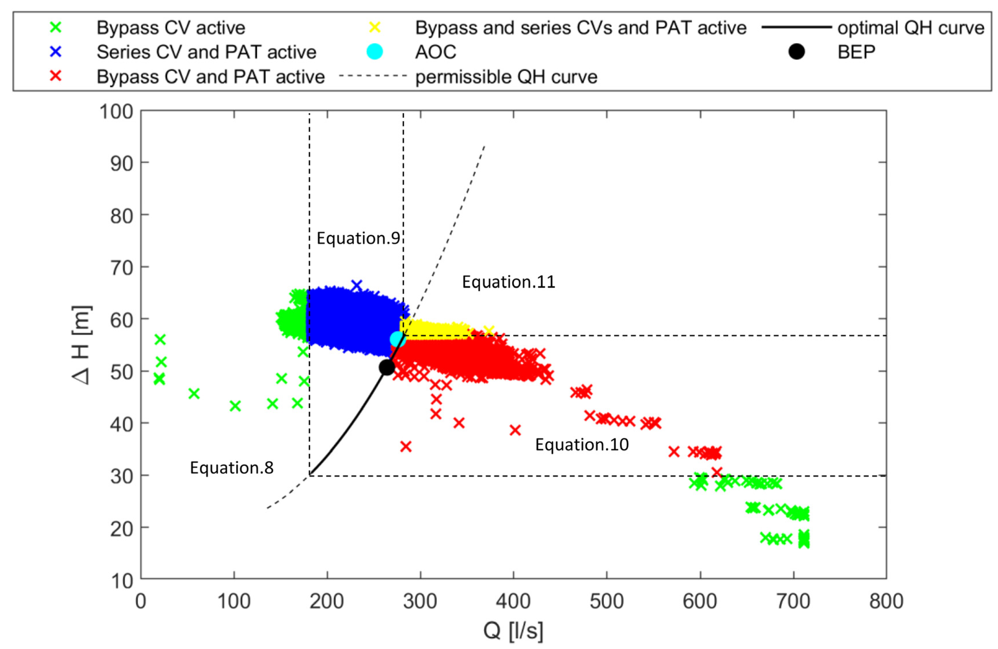
The next step was to classify all OCs according to the HR control strategy. This assesses how much flow needs to pass through the PAT (
), and how much to be bypassed in each OC to prevent excessive head loss, but also to maximize energy recovery. Based on the position of the OCs at a PRV in relation to the PAT head loss curve, all OCs can be classified in maximally four control regions (see
Figure 1). Depending in which control region an OC takes place, its
can be calculated using one of the following equations:
To assess the power generated in each OC, the previously determined values of were introduced in Equation (5). Finally, to calculate the total energy produced, the powers were multiplied with corresponding values of the recording time steps and summed.
2.2.4. Optimization Problem and Algorithm
The optimization problem described above can be formulized as follows:
For a single rotational speed
, the above problem is a nonlinear programming problem subject to nonlinear inequalities in terms of
, and upper bound for
. Because of the discontinuous nature of the objective function, a derivative free algorithm named Nelder–Mead Simplex Direct Search (NMSDS) was used to guide convergence from the initial starting point vector of design variables. As this algorithm does not incorporate the constraints, they were introduced using a penalty function (barrier method). Namely, if any of the constraints are violated, the value of
is set to zero. Because of such formulation of the penalty function, the initial starting point vector has to satisfy the constraints. The details of the set of rules that NMSDS uses to converge to the optimal solution are presented in [
12].
3. Results and Discussion
Figure 2 presents the summary of the first two steps of the experiment, i.e., the assessed AOCs at 38 PRVs included in the analysis. Among the 38 sites, the lowest average operating flow was recorded at site 9 at 2 L/s, while the highest value was recorded at site 4 at 453 L/s. The lowest average excess head was calculated for site 25 amounting to 1.5 m, while the highest value was calculated for site 38, amounting to 77 m.
Figure 2 also illustrates the variations of the OCs at the sites using the error bars whose size corresponds to the standard deviations of flow and excess head OCs. Sites 25, 31 and 33 were excluded from further analysis as the recorded excess heads were too low for the application of radial or mixed flow PATs.
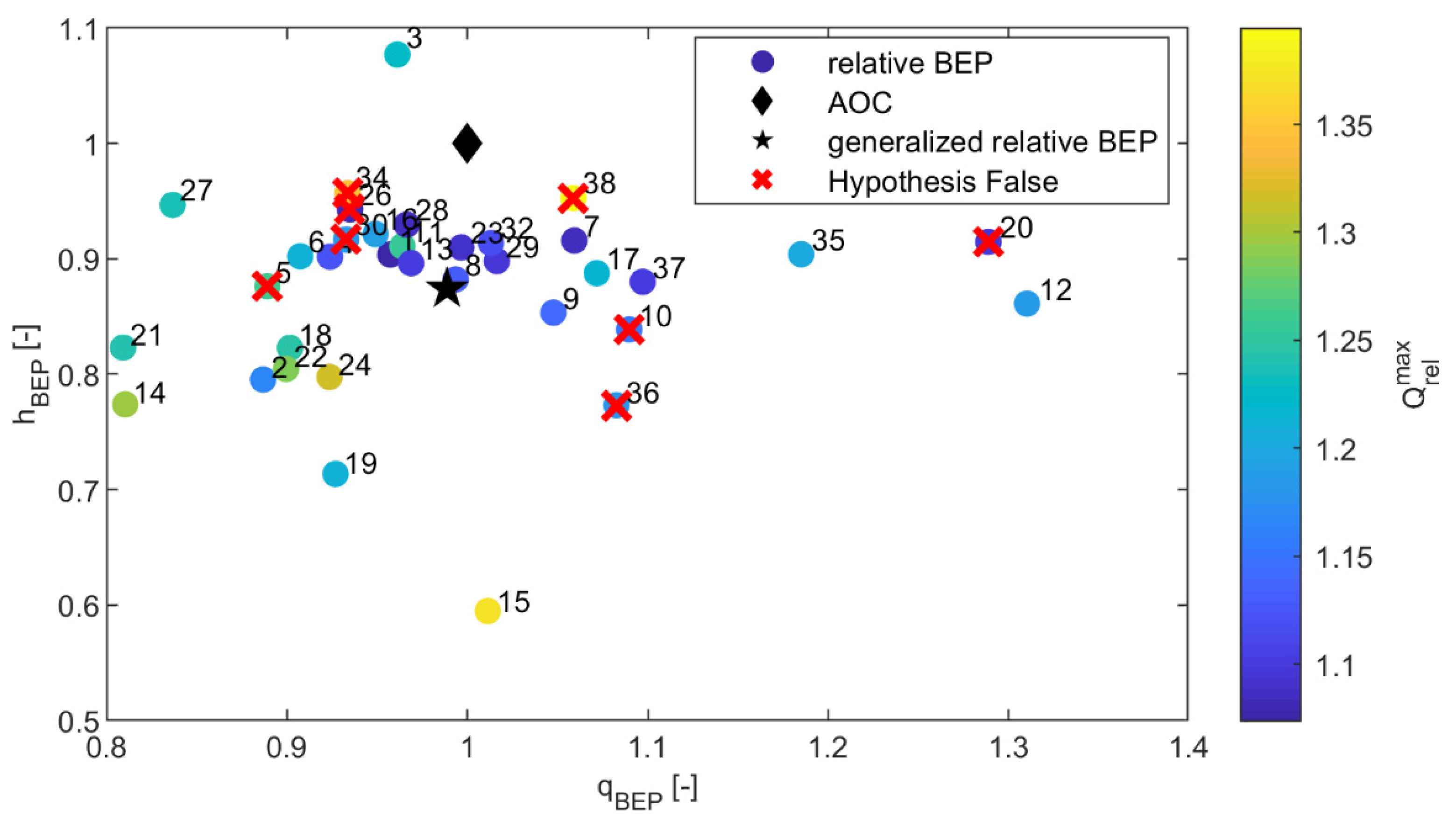
Figure 3 summarises the part of the experiment conducted in steps 3–5. The circles presented in the figure represent the relative BEP of the optimal theoretical PATs. The colours of the circles correspond to the value of the optimal
whose range is presented in the colour bar on the right. As can be seen from the colour bar, none of the values had optimal values of
below 1.07. The value of
ranges from 0.81 to 1.31, while that of
ranges from 0.59 to 1.08. The average values across 35 sites for
and
amount to 0.99 and 0.87, respectively, and represent the generalized relative BEP.
The results of the analysis conducted in step 6, i.e., the calculation of the relative distances and , suggest that, in the case of 27 out of 35 sites (77.14%), the smallest values of both distances were calculated for the same PAT models. For seven out of eight sites (27 + 7 = 34 → 34/35 = 99.14%), for which this was not the case, the models that had the shortest , had the second shortest among the PATs from the database. Only for site 20, the PAT model for which the shortest was calculated had the fourth shortest .
Finally, considering the results obtained in step 6, strictly speaking, the answer to the research question set in step 7 is negative. However, considering that the hypothesis was true for 27 out of the 35 investigated sites, and especially that the optimal PAT models from the market were the second closest to the generalized BEPs for 34 out 35 sites, it could be said that, for practical purposes, calculating the BEP of the optimal theoretical PAT is somewhat superfluous.
Of course, the results obtained in step 6 are strongly influenced by the PAT models included in the database that represented the market. In this paper, only one manufacturer (KSB) was considered, and the distances were calculated only for the PATs with the optimal speed to emulate the manual selection from the pump charts. It should be repeated that the PAT database included only the full impeller (not trimmed) models. The trimming of the impeller changes the location of the BEP of the unit and is used in the pump industry to better match the BEP of a unit to the OCs, even that its maximal efficiency is usually decreased. However, this would make sense when the OCs are relatively constant. The models with trimmed impellers would hardly achieve a better performance at sites within WDNs where the recurring part-load and over-load operation is inevitable because of the large variation in the OCs.
4. Conclusions
The aim and novelty of this paper was to investigate whether the optimal design of PATs can be generalized for sites within WDNs regardless of their variations of OCs. For this purpose, a database of 38 PRVs of a wide range of sizes and levels of variations of the OCs was assessed. The BEP of the optimal theoretical PAT for each site was calculated using the methodology proposed by [
12], which was upgraded by including an additional optimization variable representing the maximal operating flow.
The results of the experiment suggest that the selection of the optimal PAT from the market using the generalized optimal relative BEP ( = 0.99; = 0.87) would lead to the selection of the same models as when using the true theoretical optimal in the case of 27 out of 35 sites. Furthermore, the optimal PAT models had the shortest or second shortest for 34 out of 35 sites. Hence, it could be said that, for the practical purposes for manual selection (i.e., when a PAT database is not available), it is appropriate to use the generalized optimal relative BEP (multiplied with the AOC at a site) for the selection.
In this paper, the set research question was analyzed only considering the HR control strategy. In future work, this question will be analyzed for other control strategies proposed for the installation of PATs within WDNs.
Author Contributions
Conceptualization, D.M. and A.M.; methodology, D.M. and A.M.; software, D.M.; validation, D.M.; formal analysis, D.M.; investigation, D.M.; resources, D.M. and A.M.; data curation, D.M.; writing—original draft preparation, D.M., A.M. and P.W.; writing—review and editing, D.M., A.M. and P.W.; visualization, D.M.; supervision, A.M. and P.W.; project administration, A.M. and P.W.; funding acquisition, A.M. and P.W. All authors have read and agreed to the published version of the manuscript.
Funding
This paper was part funded by the European Regional Development Fund, Interreg Ireland–Wales program 2014–2020, through the Dwr Uisce project (80910).
Institutional Review Board Statement
Not applicable.
Informed Consent Statement
Not applicable.
Data Availability Statement
Data available on request.
Conflicts of Interest
The authors declare no conflict of interest.
References
- McNabola, A.; Coughlan, P.; Williams, A.P. Energy recovery in the water industry: An assessment of the potential of micro-hydropower: Energy recovery in the water industry. Water Environ. J. 2014, 28, 294–304. [Google Scholar] [CrossRef]
- García, I.F.; Novara, D.; Mc Nabola, A. A Model for Selecting the Most Cost-Effective Pressure Control Device for More Sustainable Water Supply Networks. Water 2019, 11, 1297. [Google Scholar] [CrossRef] [Green Version]
- Binama, M.; Su, W.-T.; Li, X.-B.; Li, F.-C.; Wei, X.-Z.; An, S. Investigation on pump as turbine (PAT) technical aspects for micro hydropower schemes: A state-of-the-art review. Renew. Sustain. Energy Rev. 2017, 79, 148–179. [Google Scholar] [CrossRef]
- Yang, S.-S.; Derakhshan, S.; Kong, F.-Y. Theoretical, numerical and experimental prediction of pump as turbine performance. Renew. Energy 2012, 48, 507–513. [Google Scholar] [CrossRef]
- Novara, D.; McNabola, A. A model for the extrapolation of the characteristic curves of Pumps as Turbines from a datum Best Efficiency Point. Energy Convers. Manag. 2018, 174, 1–7. [Google Scholar] [CrossRef]
- Fontana, N.; Giugni, M.; Glielmo, L.; Marini, G. Real Time Control of a Prototype for Pressure Regulation and Energy Production in Water Distribution Networks. J. Water Resour. Plan. Manag. 2016, 142, 04016015. [Google Scholar] [CrossRef]
- Carravetta, A.; Del Giudice, G.; Fecarotta, O.; Ramos, H.M. PAT Design Strategy for Energy Recovery in Water Distribution Networks by Electrical Regulation. Energies 2013, 6, 411–424. [Google Scholar] [CrossRef] [Green Version]
- Fontana, N.; Giugni, M.; Glielmo, L.; Marini, G.; Zollo, R. Hydraulic and Electric Regulation of a Prototype for Real-Time Control of Pressure and Hydropower Generation in a Water Distribution Network. J. Water Resour. Plan. Manag. 2018, 144, 04018072. [Google Scholar] [CrossRef]
- Fontana, N.; Marini, G.; Creaco, E. Comparison of PAT Installation Layouts for Energy Recovery from Water Distribution Networks. J. Water Resour. Plan. Manag. 2021, 147, 04021083. [Google Scholar] [CrossRef]
- Mitrovic, D.; Novara, D.; Morillo, J.G.; Díaz, J.A.R.; Mc Nabola, A. Prediction of Global Efficiency and Economic Viability of Replacing PRVs with Hydraulically Regulated Pump-as-Turbines at Instrumented Sites within Water Distribution Networks. J. Water Resour. Plan. Manag. 2021, 148, 04021089. [Google Scholar] [CrossRef]
- Kandi, A.; Moghimi, M.; Tahani, M.; Derakhshan, S. Optimization of pump selection for running as turbine and performance analysis within the regulation schemes. Energy 2021, 217, 119402. [Google Scholar] [CrossRef]
- Mitrovic, D.; Morillo, J.G.; Díaz, J.A.R.; Mc Nabola, A. Optimization-Based Methodology for Selection of Pump-as-Turbine in Water Distribution Networks: Effects of Different Objectives and Machine Operation Limits on Best Efficiency Point. J. Water Resour. Plan. Manag. 2021, 147, 04021019. [Google Scholar] [CrossRef]
- Stefanizzi, M.; Capurso, T.; Balacco, G.; Binetti, M.; Camporeale, S.M.; Torresi, M. Selection, control and techno-economic feasibility of Pumps as Turbines in Water Distribution Networks. Renew. Energy 2020, 162, 1292–1306. [Google Scholar] [CrossRef]
- Novara, D.; Derakhshan, S.; McNabola, A.; Ramos, H.M. Estimation of unit cost and maximum efficiency for Pumps as Turbines. In Proceedings of the IWA 9th Eastern European Young Water Professionals Conference, Budapest, Hungary, 24–27 May 2017; p. 8. [Google Scholar]
- Chapallaz, J.M.; Eichenberg, P.; Fischer, G. Manual on Pumps Used as Turbines; Vieweg & Sohn Verlagsgesellschaft mbH: Braunschweig, Germany, 1992. [Google Scholar]
| Publisher’s Note: MDPI stays neutral with regard to jurisdictional claims in published maps and institutional affiliations. |
© 2022 by the authors. Licensee MDPI, Basel, Switzerland. This article is an open access article distributed under the terms and conditions of the Creative Commons Attribution (CC BY) license (https://creativecommons.org/licenses/by/4.0/).


