Proceeding Paper

Simulation of M2 Profiles in a Channel with Rigid Emergent Vegetation †

by
Antonino D’Ippolito
* and
Francesco Calomino
Dipartimento di Ingegneria Civile, Università della Calabria, 87036 Rende, Italy
*
Author to whom correspondence should be addressed.
Presented at the International Conference EWaS5, Naples, Italy, 12–15 July 2022.
Environ. Sci. Proc. 2022, 21(1), 73; https://doi.org/10.3390/environsciproc2022021073
Published: 3 November 2022

Abstract

:
The paper presents the results relying on 12 experimental M2 water profiles observed in a flume with emergent stems in a square arrangement. The authors used a recently proposed approach to determine the drag coefficients in the flow direction. Since these showed a behavior difficult to interpret, the authors first computed for each profile the best value of the Manning coefficient for the profile simulation and then the drag coefficients. With the help of a classical dimensional analysis, a regression equation was found to predict the drag coefficients, and these were used to simulate the observed profiles with good results.

1. Introduction

Vegetation along watercourses has an important function from a hydrodynamic point of view, plays an important role in the river ecosystem, improves the landscape and has a significant recreational function [1,2,3].
Vegetation clutters up part of the river cross-section [4,5], increases roughness and reduces velocity; all this results in increased water levels and reduced water conveyance. Moreover, while the smaller average velocity on one hand reduces the erosion of the riverbed and banks, on the other one, it increases sediment deposition, which makes the water cross-sections smaller and raises the flooding risk.
Additionally, vegetation modifies the turbulence structure [6,7,8] and bed morphology [9]. Usually, in the literature, the vegetation is considered as rigid or flexible and, according to the water level, as emergent or submerged. In laboratory experiments, rigid vegetation is usually represented by cylinders of various materials and sizes [10]. Some studies have recently been carried out with reference to real vegetation in the field [11,12].
The aim of this work is to identify how the drag coefficient varies in the case of emergent rigid vegetation in a gradually varied flow profile. To this end, in Section 2, /references are made to the methods used for the calculation of the profiles in an open channel flow and to some methods used to estimate the drag coefficient, with attention on the approach proposed by Wang et al. [1]. Section 3 illustrates the equipment used to carry out the experimental tests in the presence of rigid vegetation schematized by means of cylindrical wooden sticks. In Section 4, the results of the methodology proposed by Wang et al. [1] are reported; since the drag coefficients thus obtained were difficult to interpret, the authors used another approach. They reproduced each profile with an appropriate value of the Manning coefficient and then derived continuous values of the drag coefficients. With the help of a dimensional analysis, a relationship was found that allows the experimental drag coefficient estimation. The ability of the model to simulate the experimental profiles is then verified with good results.

2. Theory

2.1. Overview and Basic Definition

Very often, it is necessary to draw the flow profile in an open channel for an assigned discharge. The main elements for the numerical calculation of a profile are summarized below, highlighting its peculiarities in the presence of emergent rigid vegetation.
To this end, reference is made to a gradually varied flow in a prismatic channel, and it is assumed that the slope of the energy grade line can be locally evaluated using a uniform flow equation with the relevant coefficient of resistance and using the local depth as the flow is locally uniform.
The total head, H , at any cross-section is
H = z + h + α V 2 2 g
in which z is the channel bed elevation; h the water depth, V the mean velocity, α the kinetic energy flux correction coefficient and g the gravity acceleration. If Equation (1) is differentiated with respect to the coordinate in the flow direction, x , the following equation is obtained
d H d x = J = i + d E d x  
in which J is the slope of the energy grade line; i is the bed slope (i.e., i = d z / d x ) and E   ( E = h + α V 2 / ( 2 g ) ) is the specific energy.
In the numerical computations of gradually varied flow profiles, the local value of the slope of the energy grade line, J , can be calculated from Manning’s equation using the local value of depth as though the flow were uniform locally [13]
V = 1 n R 2 / 3 J 1 / 2
with n the Manning’s coefficient and R the hydraulic radius. For the open channel flow without vegetation, the Manning coefficient, n , may be estimated from the mean protrusion height of the material on the bed and on the banks of the channel. However, the roughness estimate becomes complicated in the presence of vegetation elements.
In the case of vegetated channels, steady and locally uniform flow conditions require a local force balance between the flow driving mechanism and the drag term. For a given length scale d x along the streamwise direction, the flow driving mechanism is given by the weight of the fluid volume projected in the flow direction, while the resistance is given by vegetation and by the friction on the bottom and banks. In the hypothesis in which the last two can be neglected, Wang et al. [1] obtained
J = C D m D ( 1 ϕ v e g ) U 2 2 g
where C D is the drag coefficient of the cylindrical vegetation, m is the number of vegetation stems per unit area, D is the diameter of cylinders representing the vegetation,   U is the bulk velocity and ϕ v e g is the areal concentration of vegetation ( ϕ v e g = m π D 2 / 4 ) . In the case of a rectangular section of width B , the bulk velocity is defined as
U = Q B ( 1 ϕ v e g ) h
where Q is the discharge. On the basis of the above equations, the central role assumed by the drag coefficient in the profile calculation is evident.

2.2. Existing Predictors of Drag Coefficient

In the case of a single cylinder, the drag coefficient is a function of the Reynolds number, R e D ( R e D = V D / ν ). For 800 R e D < 8000 , the drag coefficient can be approximated to C D = 1.0 [14], while Cheng [15] proposed the following equation:
C D = 11 R e D 0.75 + 0.9 [ 1 e x p ( 1000 R e D ) ] + 1.2 [ 1 e x p ( ( R e D 4500 ) 0.7 ) ]  
When there is a set of cylinders, a mutual influence rises, due to the strong interaction between the wakes and between the cylinders and the wakes, in particular when the vegetation density is not small, and the value of the drag coefficient can also be significantly different from the unit. A number of studies have been carried out in this regard [2,16,17,18].
Cheng and Nguyen [19] introduces, in the hypothesis that the wall and bottom effects are negligible, the vegetation-related hydraulic radius, r v , that takes into account the density and the diameter of the vegetation, as r v = ( π / 4 ) ( ( 1 ϕ v e g ) / ϕ v e g ) D . This one, with the bulk velocity, defines the vegetation Reynolds number R e v = U r v / υ . Using experimental data from several authors (random, staggered and only two cases linear), the authors showed that the drag coefficient, relative to the bulk velocity ( C D v ), decreases monotonically with the increase in the vegetation Reynolds number and propose the following equation:
C D v = 50 R e v 0.43 + 0.7 [ 1 e x p ( R e v 15 , 000 ) ]
Wang et al. [1] analyzed the influence of vegetation on the nonuniform steady flow profile in the absence of a strong driving gradient. The authors observed eight M2-type profiles on a flume with i = 0 , in the vegetated section of lengths L between 0.52 and 0.67 m, with densities between 1% and 41.9%. The flow rate was constant Q = 3.84   L   s 1 , the upstream water depths h 0 ranged between 4.7 and 21 cm and the cylinder diameter was D = 1 cm. The numerical simulation of the profile, carried out from upstream, resulted, with the exception of the two profiles for the lower densities, in an overestimation when using Equation (6) on the drag coefficient for a single cylinder and in an underestimation when Equation (7) was used taking to account for the mutual influence of the cylinders. The authors therefore searched for an alternative expression to represent the drag coefficient. In order to reduce the noise level in the measured surface, a value of the water depth h as a function of the distance x from the beginning of the vegetated part of the channel was proposed in the form
h = c 1 l n | x c 2 | + c 3
computing the best values of c 1 , c 2 and c 3 by means of MATLAB software.
Once obtained the average flow profiles, Wang et al. [1] could compute the local drag coefficient C D by means of Equation (4). They observed a nonmonotonic pattern of the drag coefficient C D versus the stem Reynolds number R e D ; indeed, the C D increases from the inlet (low R e D ), reaching a peak value, and then decreases toward the outlets (higher R e D ). Starting from Equation (2), Wang et al. [1] arrived at the following equation for the drag coefficient
C D W = 2 g ( 1 ϕ v e g ) m D [ P A + i U 2 ]
where, however, i = 0 . In Equation (9) P and A represent the advection and pressure component, respectively, and function as C D W , of R e D . Specifically
P = S h D 2 ν 2 R e D 2
and
A = S h B ν ( 1 ϕ v e g ) g Q D R e D
with S h the slope of the free surface:
S h = h x = c 1 e x p [ c 1 c 2 Q D c 1 B ν ( 1 ϕ v e g ) R e D 1 ]
The authors show how P* A* explains the nonmonotonic behavior of C D along x for the experimental tests with 0.01 ϕ v e g 0.419 and also how, in the specific case examined characterized by constant Q , the coefficients c 1 and c 1 / c 2 depend on ϕ v e g and give relative expressions, while c 3 depends on c 1 , c 2 and the water depth in the initial section. In the case of Wang et al.’s [1] experimental tests, characterized by i = 0 , Equation (9) inserted in Equation (4) allows to reproduce in a quite correct way the detected profiles.

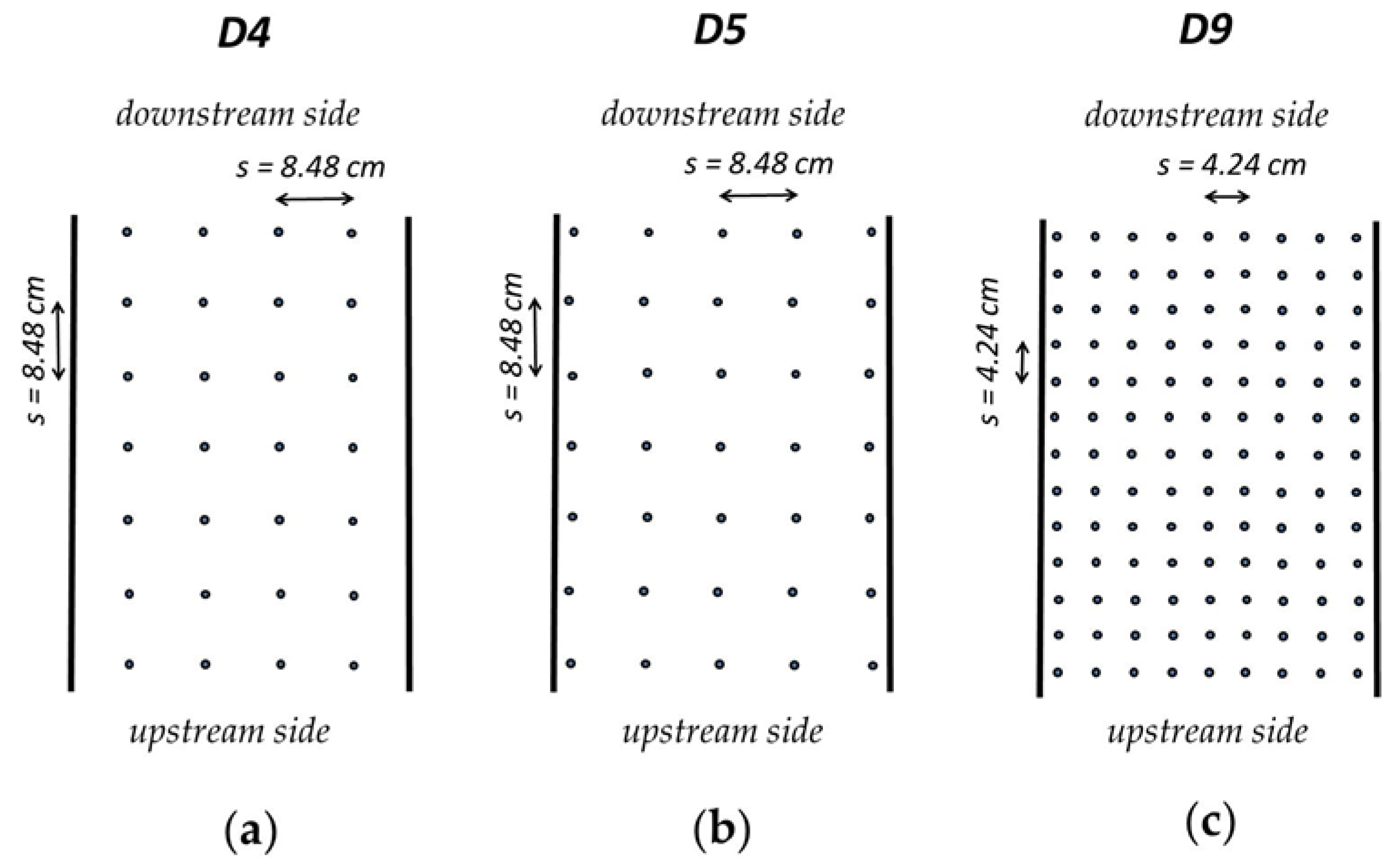
3. Experimental Data

A series of 12 tests was carried out at the “Laboratorio Grandi Modelli Idraulici” of the Department of Civil Engineering of the University of Calabria. We used a variable-slope hydraulic flume (11.13 m long), with bottom made of PVC, of width B = 0.382   m and plexiglass walls (0.21 m high). A valve on the input pipe allowed flow regulation and measurement was possible by means of a Thomson weir downstream from the flume outlet. The vegetation was modeled by means of two sets of small wooden circular cylindrical rods ( D = 0.8 and 1.0   cm ) placed in central portions of the flume (starting from x = 630 cm) of lengths variable between 1.5 and 2.2 m approximately. The rods were perpendicular to the bottom of the flume and were secured to two wooden box-structured plates.
In this work, 12 water profiles were observed, with four stem densities, achieved arranging the stems on three square meshes ( D 4 ,   D 5 ,   D 9 ) at distances of Δ x = Δ y = s = 4.24   cm and 8.48 cm (Figure 1). The vegetation density was ϕ v e g = ( π D 2 / 4 ) / ( Δ x Δ y ) = ( π D 2 / 4 ) / s 2 . Three different bed slopes ( S b ) were considered: S b 1 = 0.48 % , S b 2 = 1.35 % and S b 3 = 2.02 % , and the flow rate varied between 5.29 and 16.39 L/s.
These tests show M2 or M3M2 water profiles, observed by means of transparent measuring sticks attached to the flume wall. At the end of the section populated by stems, we could observe, in many cases, the critical depth h c = q 2 / g 3 , where q was the flow rate per unit bed width ( q = Q / B ). In some cases, even with an M2 profile, a depth other than the critical one was imposed downstream by means of a plate rotating around a hinge at the bottom of the channel.
When a M3 profile was found upstream and a M2 profile downstream, a hydraulic jump was observed between the two. Table 1 gives a summary of the performed experiments.

4. Results and Discussion

We used the same method as Wang et al. [1] to determine how the drag coefficient varies in the flow direction. In particular, for each test, the values of c 1 , c 2 and c 3 of Equation (8) that best represented the experimental profile were determined for each test. Since the water depth were known, it was possible to calculate the slope of energy grade line, and, subsequently, the values of the drag coefficients were calculated using Equation (4) and made explicit with respect to C D . Some results are shown in the following Figure 2.
While in the case of experimental tests of Wang et al. [1], the trends of C D as a function of R e D were parabolic, in our case, they were much more complex, some of them showing a maximum and a minimum while others showed increasing or decreasing approximate linear trends. These conditions make difficult to find a general law for C D and encouraged the authors to find a different way.
We started considering that, using the traditional Manning equation, it is:
J a = n 2 U a 2 R a 4 / 3
where J a , U a and R a are the average values of energy line slope, velocity and hydraulic radius, respectively, and n the Manning coefficient. For a fixed value of n , the water flow profile can be calculated using the direct step method [13]. In fact, if a downstream depth is known, an upstream one can be set and the distance between the two relative sections can be calculated using the finite difference approximation of Equation (2), which is
Δ s = Δ E i J a  
with J a given by Equation (13) and where Δ E is the difference between downstream and upstream energy by calculating E with α = 1 .
The direct step method, referred to above, has made it possible to identify, for each test, the value of n which best allows to reproduce the experimental profile. The profiles computed by this way looked to fit very well the experimental ( x ,   h ) points.
Once done this, we dispose of a continuous line representing the water profile and of the values of J for each position along it. The empirical but continuous values of C D are computed by means of Equation (4), and they look as in the following Figure 3:
Considering the following variables: stem diameter, D , distance between stem centers, s , water depth, h , liquid density, ρ , gravity acceleration, g , kinematic viscosity, ν , bulk velocity, U and drag force on N cylinders, F D , and taking into account the definition of the density of the vegetation and of the drag coefficient, based on dimensional analysis, it can be shown that C D = ψ ( ϕ v e g ,   R e h ,   R e D ) , where R e h = U h / ν is the Reynolds number computed by means of the water depth h . On the basis of the data from the 8 experimental tests (T1–T8) were carried out, the following equation was obtained
C D U C = 11.77 ϕ v e g + 0.2100   R e D 1000 0.0271 R e h 10000 0.0058
where C D U C stands for University of Calabria drag coefficient, with regression coefficient r 2 = 0.78 . Equation (15) shows that, as expected, C D U C is increasing with ϕ and R e d and decreasing with R e h .
Equation (15) allowed simulation of water profiles (also of those not used in its determination, T9–T12), once again by the direct step method, and these profiles fit very well the experimental ( x ,   h ) points. In the following Figure 4, we give some examples of them.

5. Conclusions

In the literature, several predictors of the drag coefficient used to take in account the flow resistance due to rigid vegetation have been derived under conditions of uniform flow or with reference to the action exerted on a small number of cylinders. Wang et al. [1], carrying out tests on a flat bed flume, showed how the use of the drag coefficient for an isolated cylinder or a set of cylinders under uniform flow conditions did not allow to reproduce a M2 profile. They interpolated the profiles with a logarithmic function and observed how the drag coefficient varies in the flow direction with a nonmonotonic character; indeed, it increases from the vegetated section beginning, reaching a peak value and then decreases toward the vegetated section end. The same methodology applied to experimental profiles with the bottom characterized by slopes other than zero has instead shown a different behavior with bell-shaped or quasi-linear trends, increasing or decreasing. Thus, each experimental profile was simulated using the direct step method, using for each one the best value of the Manning coefficient. Afterwards, the drag coefficients for each experimental test were calculated, noticing that they assumed a linear trend with the stem Reynolds number. On the basis of dimensional analysis, in the case of the square arrangement, the nondimensional parameters influencing the drag coefficient were identified; that is, the density, stem Reynolds number and Reynolds number computed using the water depth as the length scale, and a law was derived from the values of the eight tests performed. This was used to reproduce the 12 different experimental profiles with good results. The above law can be used to compute M2 profiles in the range of the values investigated and in the case of square arrangements.

Author Contributions

Conceptualization, F.C. and A.D.; investigation F.C. and A.D. and writing—review and editing, F.C. and A.D. All authors have read and agreed to the published version of the manuscript.

Funding

This research received no external funding.

Institutional Review Board Statement

Not applicable.

Informed Consent Statement

Not applicable.

Data Availability Statement

The data presented in this study area available on request from the corresponding author.

Conflicts of Interest

The authors declare no conflict of interest.

References

  1. Wang, W.-J.; Huai, W.-X.; Thompson, S.; Katul, G.G. Steady nonuniform shallow flow within emergent vegetation. Water Resour. Res. 2015, 51, 10047–10064. [Google Scholar] [CrossRef]
  2. Liu, M.Y.; Huai, W.X.; Yang, Z.H.; Zeng, Y.H. A genetic programming-based model for drag coefficient of emergent vegetation in open channel flows. Adv. Water Resour. 2020, 140, 103582. [Google Scholar] [CrossRef]
  3. Bonilla-Porras, J.A.; Armanini, A.; Crosato, A. Extended Einstein’s parameters to include vegetation in existing bedload predictors. Adv. Water Resour. 2021, 152, 103928. [Google Scholar] [CrossRef]
  4. Nepf, H.M. Hydrodynamics of vegetated channels. J. Hydraul. Res. 2012, 50, 262–279. [Google Scholar] [CrossRef] [Green Version]
  5. Green, J.C. Comparison of blockage factors in modelling the resistance of channels containing submerged macrophytes. River Res. Applic. 2005, 21, 671–686. [Google Scholar] [CrossRef]
  6. Caroppi, G.; Västilä, K.; Järvelä, J.; Rowiński, P.M.; Giugni, M. Turbulence at water-vegetation interface in open channel flow: Experiments with natural-like plants. Adv. Water Resour. 2019, 127, 180–191. [Google Scholar] [CrossRef]
  7. Penna, N.; Coscarella, F.; D’Ippolito, A.; Gaudio, R. Bed roughness effects on the turbulence characteristics of flows through emergent rigid vegetation. Water 2020, 12, 2401. [Google Scholar] [CrossRef]
  8. Kazem, M.; Afzalimehr, H.; Sui, J. Characteristics of turbulence in the downstream region of a vegetation patch. Water 2021, 13, 3468. [Google Scholar] [CrossRef]
  9. Penna, N.; Coscarella, F.; D’Ippolito, A.; Gaudio, R. Effects of fluvial instability on the bed morphology in vegetated channels. Environ. Fluid Mech. 2022, 22, 619–644. [Google Scholar] [CrossRef]
  10. Vargas-Luna, A.; Crosato, A.; Calvani, G.; Uijttewaal, W.S.J. Representing plants as rigid cylinders in experiments and models. Adv. Water Resour. 2016, 93, 205–222. [Google Scholar] [CrossRef]
  11. Lama, G.F.C.; Crimaldi, M.; Pasquino, V.; Padulano, R.; Chirico, G.B. Bulk drag predictions of riparian arundo donax stands through UAV-acquired multispectral images. Water 2021, 13, 1333. [Google Scholar] [CrossRef]
  12. Caroppi, G.; Västilä, K.; Järvelä, J.; Lee, C.; Ji, U.; Kim, H.S.; Kim, S. Flow and wake characteristics associated with riparian vegetation patches: Result from field-scale experiments. Hydrol. Process. 2022, 36, e14506. [Google Scholar] [CrossRef]
  13. Sturm, T.W. Open Channel Hydraulics, 2nd ed.; McGraw-Hill: New York, NY, USA, 2010; p. 546. [Google Scholar]
  14. Rowinski, P.M.; Kubrak, J. A mixing-length model for predicting vertical velocity distribution in flows through emergent vegetation. Hydrol. Sci. J. 2002, 47, 893–904. [Google Scholar] [CrossRef] [Green Version]
  15. Cheng, N.S. Calculation of drag coefficient for array of emergent circular cylinder with pseudofluid model. J. Hydraul. Eng. 2013, 139, 602–611. [Google Scholar] [CrossRef]
  16. Sonnenwald, F.; Stovin, V.; Guymer, I. Estimating drag coefficient for arrays of rigid cylinders representing emergent vegetation. J. Hydraul. Res. 2019, 47, 591–597. [Google Scholar] [CrossRef] [Green Version]
  17. D’Ippolito, A.; Calomino, F.; Alfonsi, G.; Lauria, A. Flow Resistance in Open Channel Due to Vegetation at Reach Scale: A Review. Water 2021, 13, 116. [Google Scholar] [CrossRef]
  18. D’Ippolito, A.; Calomino, F.; Alfonsi, G.; Lauria, A. Drag Coefficient of in-line emergent vegetation in open channel flow. Int. J. River Basin Manag. 2021. [Google Scholar] [CrossRef]
  19. Cheng, N.S.; Nguyen, H.T. Hydraulic radius for evaluating resistance induced by simulated emergent vegetation in open-channel flow. J. Hydraul. Eng. 2011, 137, 995–1004. [Google Scholar] [CrossRef]
Figure 1. Stem arrangements: (a) D4; (b) D5; (c) D9.
Environsciproc 21 00073 g001
Figure 2. Drag coefficients obtained following Wang et al. [1]: (a) T1; (b) T5; (c) T6; (d) T8.
Environsciproc 21 00073 g002
Figure 3. C D , computed by means of the best Manning n , versus R e D : (a) T1; (b) T5; (c) T6; (d) T8.
Environsciproc 21 00073 g003
Figure 4. Measured and predicted water levels (black line = flume bed; red circles = experimental points; blue line = computed profiles): (a) T1; (b) T5; (c) T9; (d) T12.
Environsciproc 21 00073 g004
Table 1. Characteristic parameters and results of the experimental tests.
Test n.ArrangementQ (L/s)i %d (mm) ϕ v e g ( % ) Profile Type
T1D913.552.02104.36M2
T2D916.392.02104.36M2
T3D97.901.35104.36M2
T4D910.961.35104.36M2
T5 1D913.771.35104.36M2
T6D516.312.02101.09M3-M2
T7D410.961.35101.09M3-M2
T8D98.602.0282.79M2
T9D510.921.35101.09M2
T10D95.291.35104.36M2
T11 1D914.620.4882.79M2
T12D95.772.0282.79M2
1 Experimental tests with a plate placed at the end of the channel to adjust the flow depth.
Publisher’s Note: MDPI stays neutral with regard to jurisdictional claims in published maps and institutional affiliations.

