Proceeding Paper

Direct Simulation of Micro-Component Water Consumption for the Evaluation of Potential Water Reuse in Households †

by
Tonino Liserra
,
Alessandra Bonoli
and
Vittorio Di Federico
*,‡
Department of Civil, Chemical, Environmental, and Materials Engineering (DICAM), University of Bologna, 40136 Bologna, Italy
*
Author to whom correspondence should be addressed.
Presented at the International Conference EWaS5, Naples, Italy, 12–15 July 2022.
These authors contributed equally to this work.
Environ. Sci. Proc. 2022, 21(1), 43; https://doi.org/10.3390/environsciproc2022021043
Published: 25 October 2022

Abstract

:
A study on water/energy balances at the household scale is performed using Life Cycle Assessment (LCA) to estimate Greenhouse Gas (GHG) emissions and impacts resulting from multiple scenarios incorporating various options for: (i) component sizing, (ii) energy usage, and (iii) water reuse. Sustainability indicators are evaluated to select feasible options, while reducing whole life cycle GHG emissions. Water reuse schemes using rainwater are strongly dependent on rainfall availability and require significant tank volumes. Schemes using only gray water are more compact but more energy for treatment is needed before usage. Schemes obtained by combining both options perform better in terms of reliability and sustainability.

1. Introduction

The United Nations increasingly focus their attention on water and its relationship with energy and climate change [1,2]. Water uses are strictly related to energy use in the urban cycle for operational activities and are also for the needed infrastructures provision [3]. The European Union has made these goals its own and included them in the European Commission Priorities as part of the European Green Deal [4] aimed at the achievement of climate neutrality by 2050. The European territory is extremely urbanized, with approximately 75% of the population living in urban areas [5], while the impermeable surface is above 2% of the total. It clearly emerges that in urban areas water is in itself a resource to be used for various purposes but also a source of hydrological risk due to rainwater runoff exacerbated by climate change and waterproofing of surfaces. Water-saving techniques need a combination of water reuse and meteoric water harvesting, obtained also by means of green roofs; nevertheless, all relevant technologies lead to an impact on all the sustainability dimensions that can be extended to the infrastructural domain [6]. In recent years, several solutions for water reuse [7] and rainfall harvesting [8,9] were investigated in terms of their engineering performance. Since the implementation of these solutions, the need for infrastructural adaptation has arisen, and hence some energy is used in: (i) the building phase for materials, transport, etc. (construction), (ii) the service life for operation (operation), while (iii) a part of the embedded energy can be recovered during the material recycling phase (recycling). While Life Cycle Assessment (LCA) is one of the most used tools to evaluate the environmental impacts of these solutions, in the last decades a class of mass-balance-based models has been developed such as Aquacycle [10], UWOT [11], UVQ [12], DMM [13] and WM2 [14]. These models mimic the metabolic metabolism in order to evaluate water, chemicals and energy fluxes for a UWS or the entire city [15]. The same metabolism approach can be applied at a more granular scale such as at the level of a single building. The present work proposes a simplified yet general method, the Green-Smart Technology Metabolic Model (GSTMM) in order to evaluate water savings, energy costs and infrastructural adaptations and components (tanks, pipes, filters, valves, etc.) in terms of environmental impacts; water and energy balances are coupled with LCA in order to estimate Greenhouse gas (GHG) emissions at the single household or building level. The main objective is to propose an approach able to evaluate emissions and impacts to support planning of water usage and demand management during the preliminary design phase in order to identify suitable scenarios to be subjected to more reliable LCA analysis. Materials and methods are illustrated in §2, selected indicators in §3; §4 describes the case study; results are presented in §5 and discussed in §6, while §7 reports the conclusions.

2. Materials and Methods

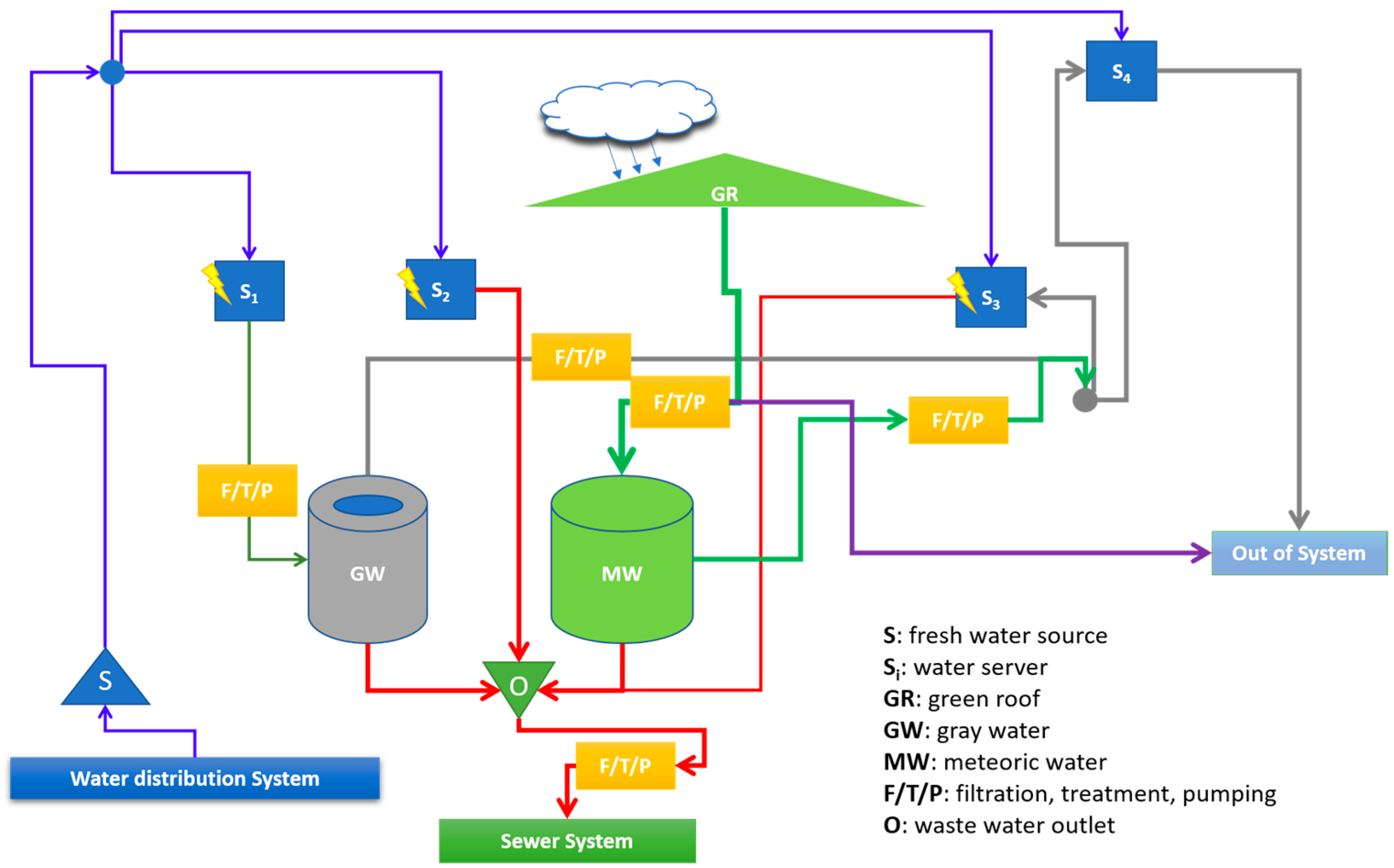
2.1. The Green-Smart Technology Metabolic Model (GSTMM)

The Green-Smart Technology Metabolic Model (GSTMM) extends the concepts already utilized by several authors [10,11,14], accounting for the peculiarities of Italian water systems. GSTMM focuses mainly on water demand management, water reuse and rainwater harvesting to reduce water withdrawals from the environment. It considers sub-daily variability of water demand inside/outside the household at the level of water appliances [16] and its direct relation with recycled water from both previous usages (SW, WM, BT, see Table 1 for abbreviations) and rainwater from roofs and/or green roofs used for non-potable usages (WC, OT, GR). The model is driven by water demand at each appliance, and evaluates material fluxes and performance indicators related to water, chemicals, and energy. It can use time series of measured water consumption and/or synthetic data from stochastic models as described in [17]. The outputs are performance indicators, time series of the calculated fluxes at multiple time and space aggregation levels, and the impacts on environment and natural resources. To describe water fluxes in a real building including several households, the presence of some essential functional elements is needed (Figure 1): (i) water demanding devices (S1, S2, Si), each representing a particular type of water use; (ii) a roof and/or green roof GR; (iii) a gray water tank GW and/or a meteoric water tank MW; (iv) filters/treatment devices/pumps (F/T/P). Finally, at least one water source S withdrawing water from the distribution system (externally modeled) and one water outlet O discharging water into the sewer system (externally modeled) are needed. Sources and outlets may be shared among several buildings, while GW, MW, and GR are shared among households belonging to the same building block. With respect to previous models, GSTMM considers all fluxes based on water origin (freshwater, gray, and rainwater). Water fluxes are evaluated using the mass conservation equation: pipes have no storage capacity; other components have storage capacity, such as water tanks; sources act as reservoirs, outlets act as sinks, and appliances act as nodes. The water balance can be computed also for households, buildings, building blocks and areas. More in detail, the starting point is the generic water appliance Si where the time series of water demand is known with given time discretization. With reference to the scheme in Figure 2a and at the time step t, the water balance for the MW is written as reported in [18]. A similar equation is adopted for the GW that is fed with water incoming from selected end-uses. It is assumed that while end-uses fed with fresh water can be used to feed GW, end-uses fed with recycled water cannot deliver water into GW. The relevant settings of the water end-uses are listed in Table 1. Each water appliance (Si) is associated to: (i) end-use type; (ii) a time series of water demand; (iii) a water type, fresh, meteoric or gray; (iv) a given fate for used water (reuse or sewer). Outputs from the model include time series for different types of water used to satisfy water demand, and energy and chemicals utilized.
Produced time series coupled with concentration of chemicals and national energetic mix are used to calculate performance indicators (PIs). With reference to Table 1, when PR is set to FW for a given end-use, then freshwater only can be used by this end-use; when PR is set to MW then the priority usage sequence is: MW, GW, FW; when PR is set to GW then the sequence is: GW, MW, FW.

2.2. Life Cycle Analysis (LCA) within GSTMM

Water, energy and fluxes of substances obtained in GSTMM can be used as input for LCA. The approach is simplified and aims at calculating emissions and impacts related to substances, energy and materials (components) necessary to implement the water reuse scheme, on the existing freshwater one, that may contain both meteoric and/or gray water. The system may be the single housing unit, a building complex, or an urban area. GSTMM calculates the total impact, for each impact category, by summing the product of the unitary LCA impact of a given component times the total quantity of such component. Therefore, specific LCA analysis needs to be carried out for all the component units (e.g., kWh of energy, kg of each substance and building material) each assumed to be a functional unit in LCA terms. Since the main sources of GHG emissions and impacts for a water system are related to the energy component in the operational phase [19], the impacts of a unit water volume can be attributed to water treatment and pumping [20]. A similar hypothesis is made for wastewater, where impacts can be estimated from total energy consumption for pumping and treatment before release into the environment. Therefore, to obtain total GHC emissions, GSTMM sums GHG emissions for all the components and for the whole energy amount as in [13] and does the same for all other impact categories. Moreover, the unit specific energy for 1 L of incoming water at the source point (S) (Figure 1) must be specified; the same for the specific energy for 1 L of wastewater leaving the area at the outlet (O). Therefore, the source S and the outlet O define the boundaries of the analysis. These simplifications are considered acceptable to use GSTMM as a tool for scenario evaluation, given the aim of providing the decision-maker with a relatively simple planning tool; then, in-depth analysis can be conducted on a selection of suitable scenarios. The environmental impact of energy derives from a study carried on by the Italian Electricity production system [21] in 2017. For each category, the impact along the entire life cycle from cradle to grave of the electricity mix is reported, referred to the functional unit 1kWh of GNC (Gross National Consumption): Climate Change (kg CO2 eq) = 4.17 × 10⁻¹; Mineral, fossil & renewable resource depletion (kg Sb eq) = 3.18 × 10⁻⁶.

2.3. Generation of Time Series of End-Use Water Demand

Water demand for all end-uses is modeled by a sequence of elementary rectangular pulses [16,17] whose arrival time is generated via a Non-Homogeneous Poisson Process (NHPP), while pulses duration and pulses intensity are simulated each with a Probability Distribution Function (PDF) that can be identified and calibrated by means of field data. Finally, the time sequence of the water pulses is described via a NHPP whose intensity function, related to the normalized consumption pattern, was obtained from the linearization of the cumulative consumption daily pattern. The parameters of the end-use demand models are adapted from [17]; they are reported in Table 2 for intensity (I) and duration (D) and each end-use in Table 1 except GR. One-year length time series are generated for all the end-uses with a 300 s time step. The required flow rate GR for garden irrigation depends on the season, temperature and meteorological events. GR varies yearly as follows: 0.019 l/s from 1 April to 30 April; 0.013 l/s from 1 May to 31 May; 0.040 l/s from 1 June to 30 June; 0.057 l/s from 1 July to 31 July; 0.058 l/s from 1 August to 31 August and 0.020 l/s from September to 30 September; GR always starts at 0:00 AM and ends at 6:00 AM every 3 days.

3. Selected Indicators for the Water System Performance

Different performance indicators (PIs) are individuated to assess the performance of meteoric water harvesting or gray water systems. The main ones among them are the tank volumetric reliability and the retention efficiency [18,22]. Given its high granularity, GSTMM allows the definition of a multitude of performance indicators at different scales, from the urban area to the single water usage. We show among those available only FW2D, GW2D and MW2D, related respectively to fresh, gray and meteoric water, which give a clear picture of how the water consumption is distributed among the three sources:
F W 2 D = 1 365 f w i 1 365 D i , G W 2 D = 1 365 g w i 1 365 D i , M W 2 D = 1 365 m w i 1 365 D i ,
where fwi, gwi and mwi are the fresh, gray and meteoric utilized water volumes in the i-th day of the year, and Di is the total daily water demand; the sum of the three synthetic indicators is equal to 1 unless water demand exceeds water availability. To show how much gray and meteoric water is used with respect to the potential water reuse demand and to the potential availability of gray and meteoric water, we propose the following indicators
E = 1 365 g w i + m w i 1 365 D i r e u , O g = 1 365 O i g w 1 365 g w i a v l , O m = 1 365 O i m w 1 365 m w i a v l ,
where Dreu is the potential demand for gray or meteoric water in the i-th day; O i g w and O i m w are the gray and meteoric water overflows from the tanks in the i-th day, g w i a v l and m w i a v l are gray and meteoric water produced in the i-th day respectively; E is the efficiency of the water reuse/harvesting system, while Og and Om give a picture of how much usable water remains unused. Noteworthy, the Oi are delivered to the treatment plant (WWTP). Two LCA impact categories are considered here: Climate Change and Mineral and Fossil & Renewable Resource Depletion in relation with energy consumption associated with water usage (see Section 2.3). To compare scenarios, energy variations are shown in Table 4 as percentage variations (∆e) with respect to the BAU (Business as Usual) scenario.

4. Case Study

We analyze a simplified system consisting of one building with a single household located on the first floor with the following end-uses: WC, DW, SW, BT, BA, WM, KT, OT, plus a garden GR having a 30 m2 surface. The total generated water demand, using the demand generator described in §2.4, is equal to 106.48 and 44.89 m3/year for in-house and garden consumption, respectively. Such water demand is typical for a four-person household in Italy. The building roof has a surface of 50 m2; a rainfall time series collected in 2014 is used, with a rain height of 893 mm. The roof acts as an impermeable surface and hydrological losses are considered. The scenarios in Table 3 are evaluated using these data and those listed in Table 1. With reference to Figure 1, water arrives at the source at a given pressure (30 m) and with a given content of energy (5.37 kJ/l) spent to produce water and deliver it to the source. In addition, water leaving the system and entering the sewer needs some energy (2.07 kJ/l) to be treated before its release to the next use (environment or agriculture). Finally, the specific energy spent to locally treat gray and meteoric water is quantified as 4.75 and 2.38 kJ/l, respectively.

5. Results

Relevant results for the simulations at building level are presented in Table 4. The values of the PIs show that the adoption of water reuse/harvesting reduces water consumption for all non-potable water usages (WC, OT, GR).

6. Discussion

The micro-component model GSTMM allows appreciating how any scenario with a gray and/or meteoric harvesting water tank leads to a reduction of the total volume abstracted from the fresh water distribution network. Gray water tanks are fed directly from the output of some water appliances (Table 1) with much more continuity than meteoric harvesting tanks; hence gray water reuse system outperforms meteoric harvesting systems when tanks have the same volume, as shown by FW2D in Table 4. Similar results are obtained with a meteoric tank of volume one order greater than the gray tank (GW2D and MW2D). A 50-L gray tank is sufficient to satisfy 36.4% of the total potential water reuse demand (E); this performance improves by increasing the gray tank size until the potential gray water demand is completely satisfied or the full gray water availability is reached.
Figure 3. Climate Change behavior across simulated scenarios.
Environsciproc 21 00043 g003
The PI Ow reflects the available gray water lost due to tank size. The water inflow to the sewer (SWR2D) measures the reduction of the water volume reaching the WWTP and positively impacts the energy needed to treat water by reducing it. In fact, all scenarios with SWRD2 < 1 imply a reduction in the energy consumption. The energy increase needed to treat water at the tank level and to lift it, with sufficient head, to the water appliance, is more than compensated by the decrease in energy usage to produce water and to treat a lower volume at the WWTP. Noteworthy, the yearly energy consumption for water production, heating and purification decreases for all scenarios with respect to BAU (2659.17 kWh/year); the same trend is obtained when heating energy (2375.56 kWh/year) is excluded from the analysis; the energy for the BAU (283.62 kWh/year) is reduced in the most favorable scenario R150-1000 by approximately 12%. Since the LCA impact is calculated on the energy consumption only, and given the assumptions in §2.3, the selected LCA impacts are proportional to the energy consumption for each scenario (Figure 3). The maximum yearly impacts are generated in the BAU scenario as Climate Change = 1108.87 kg CO2-eq; Mineral, fossil & renewable resource depletion = 8.46 × 10⁻³ kg Sb-eq. Finally, the potential energy recovered from the effluent to the sewer and in the water recovery system as heating energy (2375.56 kWh/year) is very relevant with respect the other components.

7. Conclusions

This paper presents a novel model, GSTMM, used to evaluate the effects of meteoric water harvesting and/or gray water reuse. It can be used from a single household to several buildings or urban areas and uses micro-component demand for each end-use in the households. This granularity allows calculation of quantitative PIs at all levels and clearly illustrates how water harvesting and/or gray water reuse affects fresh water usage, fluxes to the WWTP and energy consumption to manage water reuse and the harvesting system. In addition, the impact on the environment and on the natural resources can be roughly estimated based on previous LCA of the energy and materials units performed applying the urban metabolism concept. The model is applied to a hypothetical building with a single household, whose parameters derive from literature and from the authors’ expertise on the Italian water sector. Results confirm that gray water reuse requires a lower tank volume with respect to meteoric water harvesting, as production of gray water is quite constant compared to irregular meteoric events. Systems combining gray water reuse and meteoric water harvesting perform better than systems adopting a single solution. For a real building, several combinations must be explored in order to find an optimal configuration for the two tanks. Furthermore, the benefits in terms of quantitative performance must be compared in terms of costs and total impacts; the latter are associated with the installation of a recovery system and with modifications in the in-house water equipment. GSTMM can be profitably used in the planning phase as it can simultaneously run several scenarios in order to identify suitable technical suitable to be further investigated with more sophisticated and expensive tools.

Author Contributions

Conceptualization, T.L., A.B. and V.D.F.; methodology, T.L.; software, T.L.; validation, A.B. and V.D.F.; formal analysis, T.L. and A.B.; investigation, T.L. and A.B.; resources, A.B. and V.D.F.; data curation, T.L.; writing—original draft preparation, T.L. and A.B.; writing—review and editing, V.D.F.; visualization, T.L.; supervision, V.D.F.; project administration, V.D.F. All authors have read and agreed to the published version of the manuscript.

Funding

This research received no external funding.

Institutional Review Board Statement

Not applicable.

Informed Consent Statement

Not applicable.

Data Availability Statement

There are no data sharing issues since all of the numerical information is provided in the figures produced by solving the equations in the paper.

Conflicts of Interest

The authors declare no conflict of interest.

References

  1. UN General Assembly. Transforming Our World: The 2030 Agenda for Sustainable Development, 21 October 2015, A/RES/70/1. Available online: https://www.refworld.org/docid/57b6e3e44.html (accessed on 18 October 2022).
  2. UN General Assembly. Observance of World Day for Water : Resolution/Adopted by the General Assembly, 22 December 1992, A/RES/47/193. Available online: https://www.refworld.org/docid/3b00f0f224.html (accessed on 18 October 2022).
  3. Hamiche, A.M.; Stambouli, A.B.; Flazi, S. A Review of the Water-energy Nexus. Renew. Sust. Energ. Rev. 2016, 65, 319–331. [Google Scholar] [CrossRef]
  4. European Commission. The European Green Deal COM/2019/640 Final; EU Publications: Brussels, Belgium, 2019. [Google Scholar]
  5. European Environment Agency. The European Environment—State and Outlook 2020: Knowledge for Transition to a Sustainable Europe; Publications Office of the European Union: Luxembourg, 2019. [Google Scholar]
  6. Venkatesh, G.; Brattebø, H.; Sægrov, S.; Behzadian, K.; Kapelan, Z. Metabolism-modelling Approaches to Long-term Sustainability Assessment of Urban Water Services. Urban Water J. 2015, 14, 11–22. [Google Scholar] [CrossRef]
  7. Knutsson, J.; Knutsson, P. Water and Energy Savings from Greywater Reuse: A Modelling Scheme Using Disaggregated Consumption Data. Int. J. Energ. Water Res. 2021, 5, 13–24. [Google Scholar] [CrossRef]
  8. Altobelli, M.; Cipolla, S.S.; Maglionico, M. Combined Application of Real-Time Control and Green Technologies to Urban Drainage Systems. Water 2020, 12, 3432. [Google Scholar] [CrossRef]
  9. Snir, O.; Friedler, E. Dual Benefit of Rainwater Harvesting—High Temporal-Resolution Stochastic Modelling. Water 2021, 13, 2415. [Google Scholar] [CrossRef]
  10. Mitchell, V.G.; Mein, R.G.; McMahon, T.A. Modelling the Urban Water Cycle. Environ. Model. Softw. 2001, 16, 615–629. [Google Scholar] [CrossRef]
  11. Makropoulos, C.K.; Natsis, K.; Liu, S.; Mittas, K.; Butler, D. Decision Support for Sustainable Option Selection in Integrated Urban Water Management. Environ. Model. Softw 2008, 23, 1448–1460. [Google Scholar] [CrossRef]
  12. Mitchell, V.G.; Diaper, C. UVQ: A Tool for Assessing the Water and Contaminant Balance Impacts of Urban Development Scenarios. Water Sci. Technol. 2005, 52, 91–98. [Google Scholar] [CrossRef] [PubMed]
  13. Venkatesh, G.; Ugarelli, R.; Sægrov, S.; Brattebø, H. Dynamic Metabolism Modeling as A Decision-Support Tool for Urban Water Utilities Applied to the Upstream of the Water System in Oslo, Norway. Procedia Eng. 2014, 89, 1374–1381. [Google Scholar] [CrossRef] [Green Version]
  14. Behzadian, K.; Kapelan, Z. Modelling Metabolism-based Performance of An Urban Water System Using WaterMet2. Resour. Conserv. Recycl. 2015, 99, 84–99. [Google Scholar] [CrossRef]
  15. Sahely, H.R.; Dudding, S.; Kennedy, A.C. Estimating the Urban Metabolism of Canadian Cities: Greater Toronto Area Case Study. Can. J. Civ. Eng. 2003, 30, 468–483. [Google Scholar] [CrossRef]
  16. Buchberger, S.; Wu, L. Model for Instantaneous Residential Water Demands. J. Hydraul. Eng. 1995, 121, 232–246. [Google Scholar] [CrossRef]
  17. Blokker, E.; Vreeburg, J.; Van Dijk, J. Simulating Residential Water Demand with A Stochastic End-use Model. J. Water Resour. Plan. Manag. -ASCE 2010, 136, 19–26. [Google Scholar] [CrossRef]
  18. Campisano, A.; Modica, C. Selecting Time Scale Resolution to Evaluate Water Saving and Retention Potential of Rainwater Harvesting Tanks. Procedia Eng. 2014, 70, 218–227. [Google Scholar] [CrossRef] [Green Version]
  19. Filion, Y.R.; MacLean, H.L.; Karney, B.W. Life-cycle Energy Analysis of A Water Distribution System. J. Infrastruct. Syst. 2004, 10, 120–130. [Google Scholar] [CrossRef] [Green Version]
  20. Chen, Y.C. Reflecting the Environmental Cost of Greenhouse Gas Emissions from Sn Urban Water System in the Water Price. Water Environ. J. 2019, 34, 207–215. [Google Scholar] [CrossRef]
  21. Gargiulo, A.; Carvalho, M.L.; Girardi, P. Life Cycle Assessment of Italian Electricity Scenarios to 2030. Energies 2020, 13, 3852. [Google Scholar] [CrossRef]
  22. Palla, A.; Gnecco, I.; Lanza, L.; Barbera, P.L. Performance Analysis of Domestic Rainwater Harvesting Systems under Various European Climate Zones. Resour. Conserv. Recycl. 2012, 62, 71–80. [Google Scholar] [CrossRef]
Figure 1. Schematic representing a building in the GSTMM model. Symbols are defined within the Figure.
Environsciproc 21 00043 g001
Figure 2. Functional diagram for the mass balance equation in the GSTMM model: (a) Meteoric Water tank (MW); (b) Gray Water tank (GW).
Environsciproc 21 00043 g002
Table 1. Settings of the end-uses (EL = elevation above floor, PF = pressure required, PR = Preferential water type to be used, TU = average water temperature, HW = water volume served at temperature TU, RES = water volume available to reuse or sewer, REC = water volume available to reuse). The end-uses are WC = Water Closet, DW = Dish Washer, SW = Shower, BT = Bathroom Tap, BA = Bath Tub, WM = Washing Machine, KT = Kitchen Tap, OT = Outdoor Tap, GR = Garden.
End-UseEl mPF mPRTU °CHW %RES %REC %
WC2.005.0GW8.001000
DW1.005.0FW45.0501000
SW2.005.0FW45.070100100
BT1.255.0FW30.0100100100
BA1.005.0FW38.060100100
WM1.255.0FW40.050100100
KT1.255.0FW33.0801000
OT1.005.0GW8.0000
GR1.005.0GW8.0000
Table 2. Probability distribution functions (DE = deterministic, LN = lognormal, U = uniform) and statistical parameters (mean µ, standard deviation σ) for water end-use intensity (I) and duration (D).
End-UsePDF-IµσPDF-Dµσ
WCDE0.042-DE144.000-
DWU0.1400.194DE84.000-
SWU0.1200.164LN6.2340.031
BTU0.0200.064LN3.6730.179
BAU0.0800.320DE600.000-
WMU0.1400.194DE300.000-
KTU0.0700.096LN2.7340.280
OTU0.0800.120LN5.7020.066
Table 3. Simulated scenarios (scn) having different combinations of GW and MW volumes [m3].
scnGWMWscnGW MWscnGW MW
R050-0000.0500.0R000-1000.0 0.100R050-1000.050 0.100
R075-0000.0750.0R000-2500.0 0.250R075-2500.075 0.250
R100-0000.1000.0R000-5000.0 0.500R100-5000.100 0.500
R125-0000.1250.0R000-7500.0 0.750R125-7500.125 0.750
R150-0000.1500.0R000-10000.0 1.000R150-10000.150 1.000
Table 4. Performance indicators calculated for the selected scenarios (scn); all quantities defined earlier except for SWR2D = fraction of water delivered to sewer with respect to the water demand.
ScnFW2DGW2DMW2DEOwOmSWR2D∆e[%]
BAU1.0000.0000.0000.0000.0001.0000.6790.00
R050-0000.8280.1720.0000.3640.5541.0000.505−0.71
R075-0000.8120.1880.0000.3980.5131.0000.489−0.77
R100-0000.8010.1990.0000.4210.4851.0000.478−0.81
R125-0000.7920.2080.0000.4420.4601.0000.469−0.85
R150-0000.7830.2170.0000.4600.4381.0000.460−0.89
R000-1000.9370.0000.0630.1340.0000.7870.679−0.30
R000-2500.9010.0000.0990.2100.0000.6670.679−0.47
R000-5000.8630.0000.1370.2900.0000.5370.679−0.64
R000-7500.8380.0000.1620.3430.0000.4510.679−0.76
R000-10000.8170.0000.1830.3890.0000.3790.679−0.86
R050-1000.7990.1720.0300.4270.5540.9000.505−0.84
R075-2500.7660.1880.0460.4960.5130.8400.489−0.97
R100-5000.7320.1990.0690.5680.4850.7560.478−1.12
R125-7500.7030.2080.0890.6300.4600.6840.469−1.24
R150-10000.6790.2170.1050.6820.4380.6250.460−1.34
Publisher’s Note: MDPI stays neutral with regard to jurisdictional claims in published maps and institutional affiliations.

