Optimal Pressure Sensor Locations for Leak Detection in a Dutch Water Distribution Network ^†

Abstract

This paper presents a practical application of a sensitivity matrix-based methodology for determining optimal pressure sensor locations for leak detection in a water distribution network (WDN). The optimization is formulated as multi-objective, exploring the tradeoff between the minimization of the number of sensors to be installed and the maximization of the detection coverage. The methodology is applied to a real-life WDN serving the area of Seppe in the Netherlands. Close collaboration with the water utility enabled us to explore alternative designs, fine-tune the optimization problem and obtain results that are ready for practical implementation.

1. Introduction

Burst occurrences in water distribution networks (WDNs) represent a great concern for water utilities. This is because of their relation to (1) the waste of a precious resource, (2) the risk associated to water quality deterioration, (3) the risk of ensuing damages, and (4) their impact on water utility image with the public.

In recent years, a growing awareness has been shown in adopting a proactive attitude towards the possibility to detect a leak before customers notice it and call in to report it. In this perspective, the use of a sensor network (flow meters and/or pressure sensors) can help the utilities to detect and locate leakages sooner, ideally before customers point out a lower service level (i.e., low pressure, flooding and, in extreme situations, a delivery interruption). The main questions are how many sensors to install and where they should be located in order to maximize their effectiveness in allowing the water utility to recognize those events. With financial resources being constrained, the deployment of a limited number of sensors is desirable. In that regard, the use of numerical techniques can, in addition to expert judgment, be very useful in selecting the optimal number and location of sensors in a WDN.

Over the past few decades, many methodologies, based on various principles, have been developed to determine the optimal location of pressure sensors and flow meters for leak detection and localization (e.g., [1,2]). In some cases, a robust optimization formulation has been proposed by taking into account the uncertainty of some parameters, such as demand fluctuation, sensors’ accuracy, etc. (e.g., [3,4]). Nevertheless, none of the proposed methods can be considered ideal for real applications or has ever been tested for real complex systems.

In this paper, a practical application of a methodology to determine the optimal location of pressure sensors for leak detection is presented. The methodology is based on the use of the network hydraulic model for the calculation of a sensitivity matrix [5], which in turn is used to evaluate the effect of a specific leakage on the pressure in each node of the WDN. The aforementioned matrix contains the “residuals”, namely the differences in pressure between the normal operating conditions of the system and a scenario in which a leak occurs.

The optimization is formulated as multi-objective, exploring the tradeoff between the minimization of the number of sensors to be installed and the maximization of the detection coverage. The latter is expressed as the total number of users connected to the area (node) in which a pressure deviation surpasses a specified threshold when a leak occurs.

The methodology is applied to a real-life WDN serving the area of Seppe (The Netherlands). Some pressure sensors were already installed in the network prior to this research and only a limited number of sensors can be added.

An additional objective of the paper is to highlight the value of numerical optimization techniques in solving practical problems together with water utilities.

The paper is organized as follows. First, a description of the optimization problem formulation is presented, including the main modelling assumptions. A specific paragraph is also included to present an overview of the process that lead to the final formulation of the optimization problem. This was carried out in close collaboration with Brabant Water, in order to meet their specific needs, and it allowed us to create a theoretical approach suitable for real-life implementation. Then the case study is introduced, followed by the most important findings. Last, the conclusions are summarized.

2. The Approach

2.1. Context and Motivation

Brabant Water is a drinking water utility that supplies drinking water to 2.5 million inhabitants and companies in the province of North Brabant (The Netherlands). In order to detect leakages faster, Brabant Water is planning to install pressure sensors in their WDNs. The choice of pressure sensors, over flow sensors, is due to their relatively lower cost, and easier installation and maintenance. To maximize the return on this investment, it is important to think through how many sensors are needed and where they should be ideally located.

The aim of the water utility is to be able to rapidly detect (and subsequently locate) leaks before customers would notice the malfunctioning of the service, specifically during the day time hours, and call in with a complaint. The focus is, therefore, on relatively big size leaks that can quickly become visible.

The network serving the area of Seppe was selected as a pilot to determine the optimal number and location of a maximum of 20 pressure sensors, in addition to the 10 sensors that are already in place, such that the likelihood of leakage detection and covered customers is maximized. A second objective of the pilot is to investigate the value of numerical optimization techniques in selecting pressure sensor locations in a real WDN. A generic software platform for the optimization of WDNs called Gondwana [6], developed by KWR Water Research Institute, is used for this purpose. Gondwana uses EPANET [7] as a hydraulic engine and a modified genetic algorithm as the metaheuristic optimization method of choice [8,9]. In particular, the tool is able to change the decision variables (in this case the pressure sensors location) of the problem in question in a structured manner, assess the performance of each of these changes according to the objectives of the water utility, and move towards an optimal solution through an iterative process. This automatic and structured approach allows to better explore different solutions and, for instance, gain insight into the added value of each installed sensor, i.e., the trade-off between the number of sensors (costs) and the detectability of leakages (performance).

2.2. Leak Detection Methodology

The applied approach for leak detection refers to the standard theory of model-based fault diagnosis [5]. It is based on the computation of the Fault Sensitivity Matrix (FSM), obtained by a sensitivity analysis through EPANET hydraulic simulator [10]. The FSM is subsequently binarized (bFSM) with respect to a preselected pressure threshold.

Considering a single time step simulation (like in e.g., [11,12,13]), each element of the FSM (FSM_i,j), expressed in m/m³/h, is defined as the pressure residual (the difference between the nominal pressure in the model without leaks and with leaks) normalized with respect to the leakage magnitude (m³/h) and it is numerically expressed according to the following equation:

$$FS{M}_{i,j}=\frac{p_i^{f_j}-p_i}{f_j}$$

(1)

where f_j is the simulated leak magnitude (m³/h) selected accordingly to typical values that can occur in the analyzed system, $p_i^{f_j}$ and p_i are the i-node pressure (m) estimations obtained from the hydraulic model simulation with EPANET in case of a leak occurrence and the leak-free scenario, respectively (the condition–demand scenario and time window-considered in the case study for the evaluation of pressures are summarized in Paragraph 3). The difference in simulated pressures is divided by the leak magnitude in order to normalize the value, due to the possibility that some nodes could be much more sensitive to a specific leak magnitude than others. Each element of the FSM represents the sensitivity of a selected possible node-sensor location (in the row of the matrix) to the leak occurring at a specific node of the network (column of the matrix). Therefore, each row of the FSM represents an eligible sensor location, while each column is a node where a leak is simulated.

From the FSM it is possible to obtain the bFSM. For this purpose each FSM_i,j is compared with a detection threshold ($\tau$) (Equation (2)). The $\tau$ coefficient (m/m³/h) is evaluated as the ratio between the pressure threshold and the magnitude of the leakage. When the FSM_i,j is above the defined detection threshold, it is considered that the leakage occurring in the system is affecting the pressure of the node selected as a sensor location, thus 1 is assigned as a value to the element of the respective bFSM (bFSM_i,j). Otherwise, bFMS_i,j is assumed equal to 0, which means that the simulated leak is not sufficiently affecting the pressure of the node selected to locate a sensor. The pressure threshold that controls the effect of a leak on a given pressure has to be conveniently chosen, mainly based on the accuracy of the sensor that is going to be installed in the field, the plausible drop of pressure that can be caused by a certain leak-magnitude in the studied system, the minimum value of pressure variation that will be considered as a leak and then post-processed for its localization, etc.

$$bFS{M}_{i,j}=\{\begin{array}{c}1 if FS{M}_{i,j}\ge \tau \\ 0 if FS{M}_{i,j}<\tau \end{array}$$

(2)

2.3. Optimization Problem Formulation

While the main methodology for leak detection quickly was defined, the formulation of the optimization problem (objective functions, constraints and decision variables) was developed together with Brabant Water in an iterative way, to assure a good fit with the expectations of the utility and practical constraints.

The problem was formulated as multi-objective. In particular, the first objective function considered is the minimization of the number of pressure sensors to be installed in the network, in addition to the ones already in place and taking into account the maximum budget available by the utility. A second objective function is represented by the maximization of the sensors’ coverage, which was translated into three possible formulations:

• Number of detected leaks: number of leaks detected out of the total number of simulated leaks. This objective is the most simple to understand.
• Population exposure: total number of users connected to the area (node) where a specific detected leak occurs, which gives a measure of the population exposure in case of a leak occurrence. This objective puts more focus on the customers. Ideally, this would include all customers connected to an individual valve section in which the node is included.
• Pipe coverage: total length of pipes “covered”, namely the pipes for which up and downstream nodes are included in the set of leaks detected by a specific configuration of installed sensors. This objective puts more focus on the assets.

After the preliminary analysis and the verification that the three formulations had a similar performance in terms of preferred sensor locations, population exposure was chosen as the second objective function, because this was considered by Brabant Water to be more intuitive, and more suitable to explain and justify the results. The other formulations were taken into account in the post-processing step.

The decision variables are the location of the sensors. In the system, 10 sensors were already installed (at the time with a different goal than the detection of leaks). These were always included in the set of sensors during the evolution of the solutions, in order to maximize their usability for leakage detection as well.

The main constraint in the optimization problem formulation was the budget available for the installation of new sensors. This was translated into a maximum of 20 additional sensors that can be placed in the network. The former, in particular, can be selected among a total of 5814 eligible sensors locations provided by Brabant Water, which are represented by all the nodes connected to PVC pipes with a diameter of 110 mm and served by electricity supply (practical constraint).

In order to maximize the leakage detection coverage (geographical likelihood of leakage detection) with a reasonable number of pressure sensors (depending on the available budget), an optimal sensor placement methodology, based on Genetic Algorithms, was used.

2.4. Main Modelling Assumptions

The following main assumptions were considered to obtain the binarized sensitivity matrix: leakages are simulated through emitter coefficients assigned to the nodes, the magnitude of the leakages is constant (60 m³/h), leakages are assumed to occur one at a time and simulated in all the nodes of the system, and a pressure threshold (2.5 m) is considered to convert the sensitivity matrix into the binarized version.

A single time step simulation was performed, and the selection of the time of the day to be considered was defined together with Brabant Water. Namely, the idea was to be able to detect a leak occurring in a time window when customers are awake and could easily notice any disturbance in the delivery. In this regard, a sensitivity analysis considering different time steps was initially performed in order to test the effects of the selected time windows on the results of the sensor location optimization. The final choice was to use 3 PM as the time step for simulation, corresponding to the lowest demand during the diurnal time window. The latter represents the “worst-case scenario” due to less sensitivity to leakages, which means that if the sensors network can detect a leak at 3 PM, than for sure the same can been seen at other times when demand is higher.

2.5. An Insight in the Collaborative Process with the Water Utility

Before starting the project, Brabant Water already had a plan for the location of the new pressure sensors. Nevertheless, the utility decided to compare their expert judgement to the results obtained by using an optimization algorithm.

For the successful application of the proposed numerical optimization technique in the design of the pressure measurement network, an iterative cycle of design sessions was organized, where the experts from Brabant Water and KWR worked closely together to arrive at an optimal and tailored solution. During these sessions, it was possible to discuss the different versions for the optimization problem, including the choice of objectives, constraints and parameters settings, set experiments and evaluate the preliminary results out of each of the made choices. Based on this, the optimization problem was further adjusted in each cycle.

During the process, a lot of unexpected questions and answers were raised, gradually increasing the awareness of Brabant Water of the complexity of the problem, and of the influence of each parameter involved (i.e., time step of the simulation, leak magnitude, and detection threshold used to consider a drop of pressure as a real leak). For this reason, some preliminary numerical experiments were set up in order to perform a sensitivity analysis of each main variable on the resulting optimization, according to the decisions made during each meeting, before obtaining final results. Furthermore, the analysis of the preliminary results also suggested the necessity to develop a different visualization of the results in Gondwana, through coverage maps, that helped the utility in the analysis and interpretation of the outcomes of the optimized solutions.

The whole process lasted a few months and allowed KWR and Brabant Water to gain insights on how to improve the collaboration for the implementation of numerical optimization techniques in supporting water utilities in solving practical problems.

3. The Case Study of Seppe

The methodology proposed for the optimization of the location of pressure sensors was applied to the water distribution system serving a total of 43,143 customer connections in the area of Seppe, in the province of North Brabant in the Netherlands.

In the hydraulic model, the supply of the network is simulated through a reservoir and a tank, both connected to a pumping station.

In order to reduce the search space and, consequently the computational time, a first skeletonized version of the system was provided by Brabant Water, in which branched pipes and pipes with a diameter below 50 mm were removed, while sets of pipes with the same characteristics were replaced with equivalent single pipes. After the preliminary analysis, the choice to modify one of the objective functions according to specific requests made by Brabant Water led to the common decision to use a partially-skeletonized version of the network. This was obtained from the initial skeletonized model, with the addition of the branched pipes and considering also a new pipe that will be placed in the near future.

The demand pattern assigned to the residential customers, with a time step of 5 min, represents 10% more than the average day (average demand multiplier = 1.1). The time step considered for the hydraulic calculations is 1 h and the analysis is a single time step simulation.

More details on the hydraulic model can be found in

Table 1. Values of the parameters used to obtain the final results.

Parameter	Value
Daily flow (m3/d)	43,046
Number of simulated leaks (number of nodes)	19,410
Number of demand nodes	8167
Total number of connections	43,143
Total pipes length	944.5 km
Objective function 1	N. sensors
Objective function 2	N. connections
Decision variables (min–max)	1–20 new sensors locations
Post-processing objective evaluation	N. detected leaks Pipes length
Leak magnitude	60 m3/h
Pressure threshold	2.5 m
Eligible meters locations	5818
Single time step simulations	3 PM

.

4. Results

The results obtained for the multi-objective optimization problem are shown through the Pareto front in Figure 1. Each point of the Pareto represents a certain set of sensors (solution), always including the 10 pressure sensors already installed in the system.

In the context of the simulation, from an initial coverage of 11,441 connections, obtained with the initial configuration, a maximum of 22,967 out of 43,143 connections can be considered covered if the 30-sensors solution is used. Total coverage of the occurring leaks cannot be ensured due to the fact that for the considered leak magnitude, the drop of pressure (at the nodes nearby the leak but also at the node where the leak was simulated) is often below the considered threshold. Furthermore, in some areas of the network, even if the drop of pressure is sufficient to detect a leak, there were no nodes eligible for sensor placement (constraint).

The same results are also presented in

Table 2. Value of the optimized solutions in terms of the three objective function formulations.

N. Sensors	N. Connections	N. Detected Leaks	Pipe Length (km)
10	11,441 (26.5%)	5077 (26.2%)	236.75 (25.1%)
11	12,815 (29.7%)	5663 (29.2%)	254.19 (26.9%)
12	14,075 (32.6%)	5998 (30.9%)	267.70 (28.3%)
13	15,071 (34.9%)	6452 (33.2%)	287.70 (30.5%)
14	16,049 (37.2%)	6841 (35.2%)	300.39 (31.8%)
15	17,003 (39.4%)	7234 (37.3%)	320.35 (33.9%)
16	17,924 (41.5%)	7557 (38.9%)	328.16 (34.7%)
17	18,701 (43.3%)	7885 (40.6%)	339.75 (36%)
18	19,407 (45.0%)	8277 (42.6%)	360.78 (38.2%)
19	19,889 (46.1%)	8490 (43.7%)	374.02 (39.6%)
20	20,344 (47.2%)	8612 (44.4%)	377.57 (40%)
21	20,740 (48.1%)	8700 (44.8%)	379.94 (40.2%)
22	21,111 (48.9%)	8817 (45.4%)	382.83 (40.5%)
23	21,468 (49.8%)	9112 (46.9%)	405.30 (42.9%)
24	21,785 (50.5%)	9161 (47.2%)	407.17 (43.1%)
25	21,957 (50.9%)	8988 (46.3%)	393.38 (41.6%)
26	22,208 (51.5%)	9137 (47.1%)	400.88 (42.4%)
27	22,298 (51.7%)	9216 (47.5%)	410.36 (43.4%)
28	22699 (52.6%)	9331 (48.1%)	415.01 (43.9%)
29	22,868 (53.0%)	9371 (48.3%)	413.73 (43.8%)
30	22,967 (53.2%)	9405 (48.5%)	415.55 (44%)

, where for each set of sensors (solution optimized with the number of connections) the corresponding values of the detected leakages and the covered pipe length (calculated during the post-processing) are reported. The same table shows the coverage in terms of percentage with respect to the total amount of connections (43,143), total simulated leaks (19,410) and total pipe length (944.5 km), respectively. The highest improvements are obtained from the 11-sensors solution until the 18-sensors solutions, for which the number of covered connections increases about 2–3% with each added sensor. From the 19-sensors solution, the coverage contribution starts to decrease from 1% down to 0.2%. When the maximum number of sensors that can be installed is considered, a respective coverage of 53.2% is reached in terms of number of connections, while the detected leaks and the pipe length are of about 48.5% and 44%, respectively.

By looking at the results in terms of number of detected leaks and pipe length, the values are not continuously increasing, but tend to have a variable behavior. For instance, from the solution with 24 sensors to the one with 25, the two formulations assume a decreased value, from 47.2% to 46.3% and from 43.1% to 41.6%, respectively. The reason for this behavior is that the solutions were optimized for the number of connections, while the other formulations were evaluated only in the post-processing.

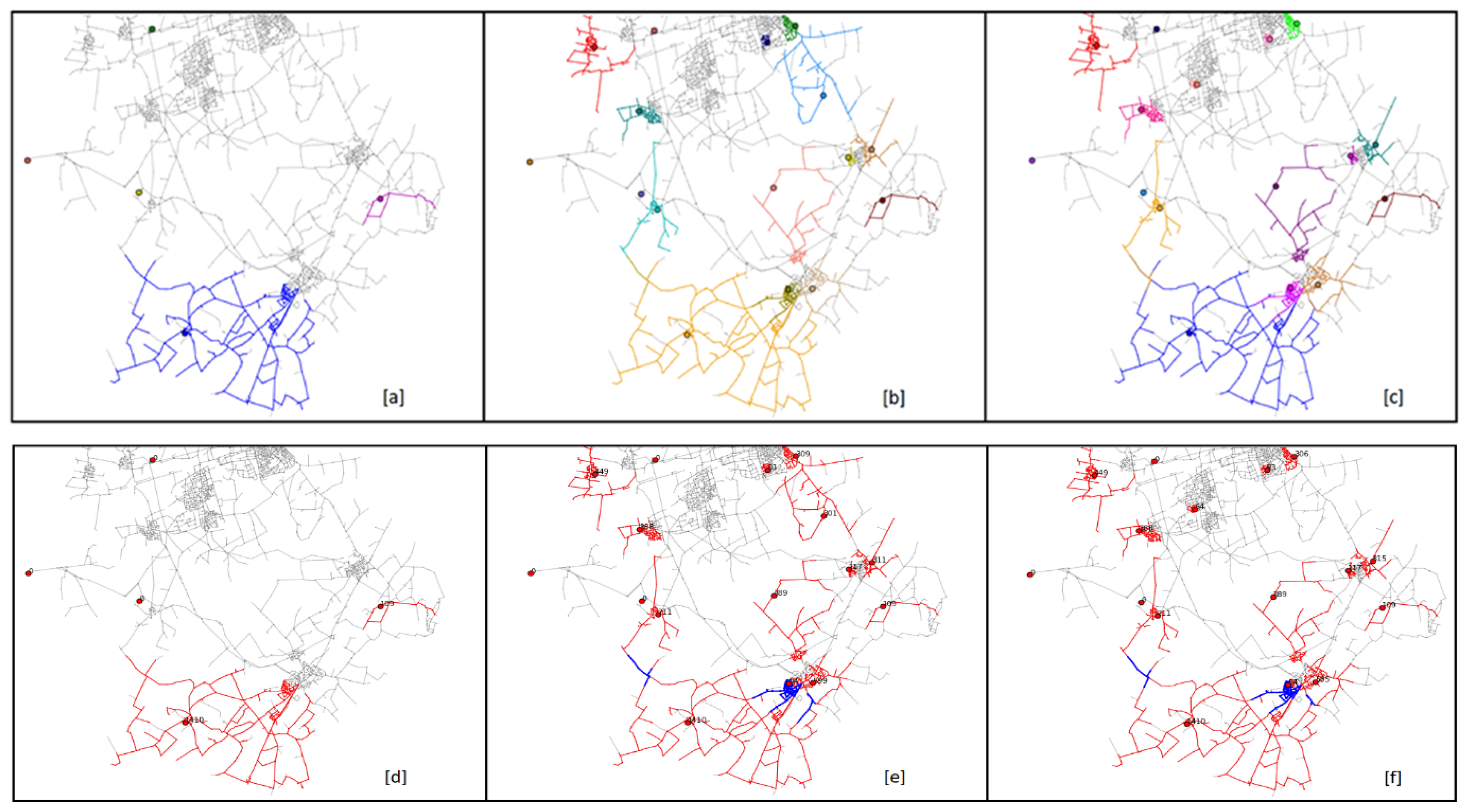
In order to show clearly the benefit that each additional sensor installed in the network would bring in terms of leak detection, the coverage obtained by the sensors is illustrated through maps: either as a distinction of the contribution of each sensor (see Figure 2a–c) or to show the existing coverage overlapping (see Figure 2d–f). The maps allow us to visualize, for each solution, where the sensors are located and show those pipes in which leakages are “detected” for the specified set of sensors (i.e., pipes included between two nodes where the simulated leaks are detected). This is highlighted in the coverage map with different colours for each senor (the sensor and the pipes covered by that sensor have the same colour), while in the overlapping coverage map, the blue indicates the overlapping (pipes covered by more than one sensor) and red represents those pipes covered only by one sensor. The pipes of the WDN in grey are the ones not covered by the considered solutions.

In Figure 2, only a small portion of the network is shown to guarantee privacy protection. Among the initial 10 sensors, only five are visible (Figure 2a–d). In Figure 2b–e and Figure 2c–f the solutions of the Pareto front with 24 and 25 sensors in total, respectively, is represented as an example, but only the effect of some of the additional sensors is shown.

Among the actual pressure sensors configuration (Figure 2a–d), there are some that are effective in the specific simulation conditions analyzed, despite being installed for reasons that differ from the leak detection purpose. In particular, six sensors (two of them visible in Figure 2a–d) out of ten contribute to leak detection. The four sensors that have a null coverage (three are visible in Figure 2a–d) are the ones installed in the central area of the network, corresponding to the location of a water treatment plant, and of a control valve and a pressure meter located on feeding pipes for two adjacent areas. The detection coverage overlapping occurs only for two sensors in the northern part of the system, not visible in Figure 2d.

It is noted that by increasing the number of sensors installed in the network, the chance to have overlapping on the same detected leaks also tends to increase.

It is important to stress that, from the analysis of the various solutions, mainly carried out through the coverage maps, some sensors seem to be part of all them, while there is a certain number that tends to change from one solution to another. This is clearly visible, for example, in the 25-sensors solution (Figure 2c). The latter is characterized by a different allocation of sensors respect to the 24-sensors solution (Figure 2b). This means that, in the perspective of a gradual investment on the installation of new sensors, the configuration (set of sensors) should be selected upfront, accepting that for a certain time (till the installation of all sensors is completed) the performance will be below the one expected to be achieved with the full configuration.

5. Conclusions

The main novelty presented in this paper is represented by the practical application of a leak detection method based on a sensitivity matrix, showing the obstacles that can be encountered when dealing with real systems and how to collaborate with water utilities, not just to find an optimal solution, but an optimal solution that takes into account real necessities and constraints. Indeed, the results show the value of applying powerful tools such as numerical optimization techniques to real-life problems which are too complex to be solved only by engineering judgement: it saves time, allows the utilities to explore a number of solutions much higher than could be manually tested and may prevent investment in sensors at unviable locations. It is important to mention that the expert judgment remains fundamental for the correct use of the tool, for the critical analysis of the obtained results and for the final decision.

The results of the approach used in the presented process highlight the importance of close collaboration with the water utility to enable the exploration of alternative designs, fine-tune the optimization problem and obtain results which can be implemented in practice.