Spatio-Temporal Optimal Interpolation of Aerosol Optical Depth Observations Using a Chemical Transport Model ^†

Abstract

To estimate the spatial and temporal distribution of aerosol optical depth (AOD), we used the optimal interpolation (OI). In OI, observational data and a model forecast are linearly combined according to their relative accuracies. Weight coefficients are chosen to minimize the mean-square error in the estimate. To obtain weight coefficients, correlations between model errors in the different grid points are used. In classical OI, only spatial correlations are considered. We used spatial and temporal correlation functions. To obtain error statistics, we used observations from European stations of ground-based sun photometers, the Aerosol Robotic Network (AERONET), and simulations by a chemical transport model GEOS-Chem, assuming a negligible error of AERONET AOD observations. The estimates of the daily mean AOD distribution over Europe are obtained. The reduction of the root-mean-square error of the AOD estimate based on the OI method in comparison with the GEOS-Chem model results is discussed.

1. Introduction

Atmospheric aerosol has a considerable impact on air quality and climate. One of the important characteristics of atmospheric aerosol is aerosol optical depth (AOD), which is a measure of light extinction by aerosol. The atmospheric column integrated aerosol load can be derived from AOD observations. A global ground-based network of sun and sky photometers, the Aerosol Robotic Network (AERONET), provides AOD data with low uncertainty [1,2,3,4,5]. However, AERONET observations are sparse in space and time. Chemical transport models can fill in observational gaps. Model simulations provide values of AOD at all cells of a regular grid over the domain of interest. A variety of models is used to describe aerosol optical properties, including AOD [6,7,8,9,10]. The drawback of the models is a large uncertainty. To obtain a likely true estimate of the spatial and temporal distribution of AOD, data assimilation can be applied. Data assimilation is a technique of combining observational data with model simulation outputs. Data assimilation approaches are commonly divided into optimal interpolation (OI) [11,12,13], Kalman filtering (KF) [14,15,16], and variational methods [17,18,19]. All of these approaches are based on the minimum mean-square error principle of the estimation theory. Each method has advantages and disadvantages depending on specific applications. OI estimates a value of interest in a grid point through a weighted linear combination of observational and modeled data at the point in question and neighboring observational points, according to the accuracies of the data used. Weighting coefficients are chosen to minimize the mean-square error in the estimate. To obtain weighting coefficients, correlations between model errors in the different grid points are used. A single correlation function is estimated from available data, assuming homogeneity and isotropy of the field. The model error statistics are assumed to be stationary. KF is a sequential data assimilation scheme. KF is a two-step process: the forecast and the analysis. The forecast is made using a dynamical model, in which the estimate obtained in a previous time step is incorporated. The analysis is the same as OI. A forecast error covariance updated in every time step is used instead of a single model error covariance. This allows reducing the mean-square error in the estimate in comparison with OI. However, if the temporal gaps are present in the observational data, there is no improvement in comparison with OI, because the values being estimated converge too quickly to the model trajectory [20]. Variational methods are based on minimizing an objective function proportional to the square of the distance between the estimate and both the model and the observations. Under some commonly used assumptions, the three-dimensional variational method (3D-Var) is equivalent to OI [21]. Difference is only in the method of the solution. In the four-dimensional variational approach (4D-Var), the minimization of the objective function is carried out over a time window. The numerical cost of 4D-Var is very high. OI is much less computationally expensive than KF and 4DVar methods.

In classical OI, only spatial correlations are considered. The method can be extended to include time dimension by using spatial and temporal correlations. The use of spatio-temporal optimal interpolation (STOI) allows filling in not only spatial, but also temporal gaps in observations, and improving the accuracy of the method. STOI was used in ocean sciences in [22,23]. In [24] we used STOI combining AERONET observations and chemical transport model GEOS-Chem [25,26] calculations, for the estimation of the distribution of AOD at 870 nm over the eastern European region. In the present work, we assimilated AERONET AOD at wavelengths of 440, 675, and 870 nm using STOI to obtain the distribution of total AOD over Europe.

2. Materials and Methods

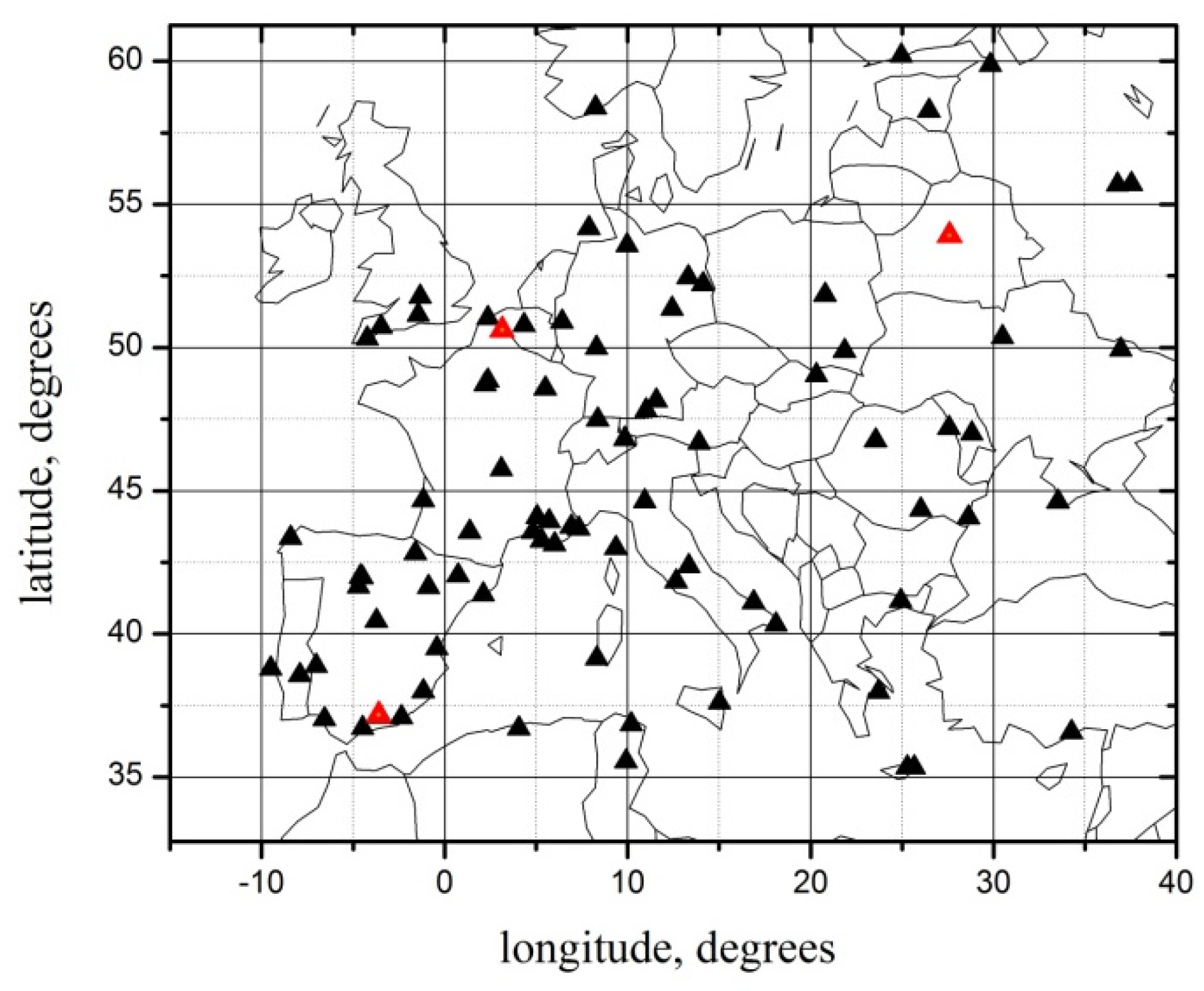
2.1. AERONET Observations

One of the widely used sources of atmospheric aerosol data is observations by a ground-based network of sun and sky photometers, AERONET. The network consists of more than 500 sites located throughout the world. Photometers provide measurements of direct solar and diffused sky radiation at a number of wavelengths. The AERONET retrieval algorithm [3] derives AOD and other integrated aerosol properties from direct and diffuse radiation measurements. AERONET observations are often considered as a standard for column aerosol properties. An uncertainty of AERONET observations of AOD is approximately 0.01 for wavelengths > 440 nm [4,5]. In this paper, we used AERONET Version 3, Level 2 (cloud-screened and quality-assured) daily averaged total AOD data.

2.2. GEOS-Chem Simulation

GEOS-Chem is a global three-dimensional chemical transport model. The GEOS-Chem model is developed and used by research groups worldwide as it is applicable to a broad range of atmospheric composition problems. The model input includes meteorological data and inventories of emissions. The archived meteorological fields are derived from the Goddard Earth Observing System (GEOS) [27]. GEOS-Chem uses the Harvard–NASA Emissions Component (HEMCO) [28] to calculate emissions from different databases. The model output is a set of quantities, such as tracer concentrations, in every grid cell and others including the AOD of major aerosol components at a number of wavelengths with a transport time step of 15 min. For calculating AOD, GEOS-Chem combines aerosol species into groups according to their optical properties: sulphate–nitrate–ammonium; size fractions of mineral dust; sea salt in accumulation and coarse modes; black carbon; organic aerosols.

In the present work, we used a nested regional application of GEOS-Chem version v12.1.1. The simulation was performed at 0.25° latitude × 0.3125° longitude horizontal resolution and 47 vertical σ-layers up to ~80 km. We calculated daily averaged AOD at 440, 675, and 870 nm as these are standard reference wavelengths in AERONET products. Optical depths of the above-mentioned individual aerosol groups in every 3D grid cell were summarized to obtain the optical depth of the total aerosol in the cell. The optical depths of the total aerosol in every vertical layer for the given horizontal grid cell were summarized to yield the total column AOD.

2.3. Spatio-Temporal Optimal Interpolation

In the OI scheme, an analyzed state is related to the forecast state by the equations:

$$x^a=x^b+K[y-H(x^b)],$$

(1)

$$K={\mathrm{BH}}^{\mathrm{T}}{({\mathrm{HBH}}^{\mathrm{T}}+R)}^{-1},$$

(2)

were x^a is a vector containing estimated values at regular grid points, x^b is a vector containing values calculated by a model at regular grid points, y is a vector containing values of observations at the observational points, K is a matrix containing weighting coefficients, H is an observation operator providing the link between the analysis variables and the observations, B is a covariance matrix of model errors, and R is a covariance matrix of observational errors. The matrix of weighting coefficients, K, is to be determined by minimizing the mean-square error in the estimate. Equations (1) and (2) define the optimal linear estimator under the assumption that the errors are unbiased, the observational errors are uncorrelated, and observational and model errors are mutually uncorrelated. In OI, not all available observations are considered: only those lying in the vicinity of the point being updated.

We applied STOI to estimate AOD in Europe during the period 2015–2016. We considered data from 88 European AERONET sites. The layout of the region and location of the sites are shown in Figure 1.

As model AOD uncertainty [29] is significantly larger than AERONET AOD uncertainty, we assumed the observations to be perfect.

Prior to the implementation of the STOI, we compared GEOS-Chem simulated AOD with AERONET observations. The comparison revealed a bias of −0.032 for 440 nm, −0.025 for 675 nm, and −0.024 for 870 nm. Moreover, the dispersion of AERONET AOD turned out to be significantly larger than that of GEOS-Chem-simulated AOD for each wavelength. To correct the discrepancy, we used linear regression. We then applied STOI using the corrected values of GEOS-Chem simulated AOD.

To implement STOI, a spatial and a temporal correlation functions should be known. We obtained correlation curves by fitting them to the points presenting correlation coefficients of the model-minus-observation pairs of AOD at two spatial or temporal locations, depending on the distance between them. We then modelled the obtained correlation curves by analytic functions. We choose exponential functions with argument kd where, for the spatial correlation function, d is the distance in kilometres, k = 0.002 for 440 nm, 0.0025 for 675 nm, and 0.003 for 870 nm; for the temporal correlation function, d is the time interval in days, k = 0.4 for 440 nm, 0.45 for 675 nm, and 0.5 for 870 nm. The separability of spatial and temporal correlations is assumed.

3. Results and Discussion

Using STOI, we obtained the estimate of the distribution of the daily averaged AOD in Europe for the period 2015–2016. To validate the results, we compared them with independent AERONET observations. We excluded AERONET sites Granada, Lille, and Minsk (see Figure 1) from the assimilation scheme and performed STOI for July 2015 using data from the 85 remaining sites. We obtained estimates of AOD at each of the excluded sites and calculated root-mean-square errors of the estimates using AOD observations at those sites, assuming a negligible error of AERONET AOD observations. We then calculated root-mean-square errors of model-simulated AOD at those sites. The results of the comparison are shown in

Table 1. Root-mean-square errors of the aerosol optical depth (AOD) calculated using GEOS-Chem and assimilated using spatio-temporal optimal interpolation (STOI) as compared to AOD observed by AERONET.

Wavelength nm	Granada		Lille		Minsk
	GEOS-Chem	STOI	GEOS-Chem	STOI	GEOS-Chem	STOI
440	0.127	0.046	0.091	0.055	0.090	0.068
675	0.113	0.034	0.057	0.032	0.047	0.036
870	0.111	0.034	0.046	0.023	0.032	0.026

.

The comparison shows that, averaged over three wavelengths, the reduction in root-mean-square error of the estimate after STOI is 68% for Granada, 45% for Lille, and 22% for Minsk. The best improvement among those three sites is achieved for Granada. This is due to the presence of a number of AERONET stations located close to Granada, and the large errors in the GEOS-Chem calculations for Granada during the period under consideration. A relatively poor improvement occurs for Minsk. The eastern European region is characterized by sparse observations. The dominant source of errors in assimilated AOD in this region arises from uncertainties in the model results.

Generally, STOI is a computationally efficient technique able to decrease the errors significantly in comparison with the model calculations.

References

1. Holben, B.N.; Eck, T.F.; Slutsker, I.; Tanre, D.; Buis, J.P.; Setzer, A.; Vermote, E.; Reagan, J.A.; Kaufman, Y.J.; Nakajima, T.; et al. AERONET—A federated instrument network and data archive for aerosol characterization. Remote Sens. Environ. 1998, 66, 1–16. [Google Scholar] [CrossRef]
2. NASA; Goddard Spase Flight Center; AERONET; Aerosol Robotic Network. Available online: https://aeronet.gsfc.nasa.gov/ (accessed on 25 May 2022).
3. Dubovik, O.; King, M.D. A Flexible Inversion Algorithm for Retrieval of Aerosol Optical Properties from Sun and Sky Radiance Measurements. J. Geophys. Res. 2000, 105, 20673–20696. [Google Scholar] [CrossRef]
4. Eck, T.F.; Holben, B.N.; Reid, J.S.; Dubovik, O.; Smirnov, A.; O’Neill, N.T.; Slutsker, I.; Kinne, S. Wavelength Dependence of the Optical Depth of Biomass Burning, Urban and Desert Dust Aerosols. J. Geophys. Res. 1999, 104, 31333–31349. [Google Scholar] [CrossRef]
5. Holben, B.N.; Tanre, D.; Smirnov, A.; Eck, T.F.; Slutsker, I.; Abuhassan, N.; Newcomb, W.W.; Schafer, J.; Chatenet, B.; Lavenue, F.; et al. An Emerging Ground-Based Aerosol Climatology: Aerosol Optical Depth from AERONET. J. Geophys. Res. 2001, 106, 12067–12097. [Google Scholar] [CrossRef]
6. Chin, M.; Ginoux, P.; Kinne, S.; Torres, O.; Holben, B.N.; Duncan, B.N.; Martin, R.V.; Logan, J.A.; Higurashi, A.; Nakajima, T. Tropospheric Aerosol Optical Thickness from the GOCART Model and Comparisons with Satellite and Sun Photometer Measurements. J. Atmos. Sci. 2002, 59, 461–483. [Google Scholar]
7. Morcrette, J.-J.; Boucher, O.; Jones, L.; Salmond, D.; Bechtold, P.; Beljaars, A.; Benedetti, A.; Bonet, A.; Kaiser, J.W.; Razinger, M.; et al. Aerosol Analysis and Forecast in the European Centrefor Medium-Range Weather Forecasts Integrated Forecast System: Forward Modeling. J. Geophys. Res. 2009, 114, D06206. [Google Scholar] [CrossRef]
8. Carnevale, C.; Finzi, G.; Mannarini, G.; Pisoni, E.; Volta, M. Comparing Mesoscale Chemistry-Transport Model and Remote-Sensed Aerosol Optical Depth. Atmos. Environ. 2011, 45, 289–295. [Google Scholar] [CrossRef]
9. Meier, J.; Tegen, I.; Mattis, I.; Wolke, R.; Alados Arboledas, L.; Apituley, A.; Balis, D.; Barnaba, F.; Chaikovsky, A.; Sicard, M.; et al. A Regional Model of European Aerosol Transport: Evaluation with Sun Photometer, Lidar and Air Quality Data. Atmos. Environ. 2012, 47, 519–532. [Google Scholar] [CrossRef]
10. Li, S.; Yu, C.; Chen, L.; Tao, J.; Letu, H.; Ge, W.; Si, Y.; Liu, Y. Inter-Comparison of Model-Simulated and Satellite-Retrieved Componential Aerosol Optical Depths in China. Atmos. Environ. 2016, 141, 320–332. [Google Scholar] [CrossRef]
11. Gandin, L.S. Objective Analysis of Meteorological Fields; Gidrometeorol. Izd.: Leningrad, Russia, 1963; (English translation by Israel program for scientific translations, Jerusalem). [Google Scholar]
12. Lorenc, A.C. A Global Three-Dimensional Multivariate Statistical Analysis Scheme. Mon. Weather Rev. 1981, 109, 701–721. [Google Scholar] [CrossRef]
13. Daley, R. Atmospheric Data Analysis; Cambridge University Press: Cambridge, UK, 1991. [Google Scholar]
14. Kalman, R.E. A New Approach to Linear Filtering and Prediction Problems. J. Basic Eng. 1960, 82, 35–45. [Google Scholar] [CrossRef]
15. Kalnay, E. Atmospheric Modeling, Data Assimilation and Predictability; Cambridge University Press: Cambridge, UK, 2002. [Google Scholar]
16. Evensen, G. Data Assimilation: The Ensemble Kalman Filter; Springer: Berlin/Heidelberg, Germany, 2009. [Google Scholar]
17. Sasaki, Y. An Objective Analysis Based on the Variational Method. J. Meteorol. Soc. Japan 1958, 36, 77–88. [Google Scholar] [CrossRef]
18. Talagrand, O. A Study on the Dynamics of Four-Dimensional Data Assimilation. Tellus 1981, 33, 43–60. [Google Scholar] [CrossRef]
19. Fisher, M.; Lary, D.J. Lagrangian Four-Dimensional Variational Data Assimilation of Chemical Species. Q. J. R. Meteorol. Soc. 1995, 121, 1681–1704. [Google Scholar]
20. Tombette, M.; Mallet, V.; Sportisse, B. PM10 Data Assimilation over Europe with the Optimal Interpolation Method. Atmos. Chem. Phys. 2009, 9, 57–70. [Google Scholar] [CrossRef]
21. Lorenc, A.C. Analysis Methods for Numerical Weather Prediction. Q. J. R. Meteorol. Soc. 1986, 112, 1177–1194. [Google Scholar] [CrossRef]
22. Sentchev, A.; Yaremchuk, M. Monitoring tidal currents with a towed ADCP system. Ocean Dyn. 2016, 6, 119–132. [Google Scholar] [CrossRef]
23. Stanev, E.V.; Ziemer, F.; Schulz-Stellenfleth, J.; Seemann, J.; Staneva, J.; Gurgel, K.-W. Blending Surface Currents from HF Radar Observations and Numerical Modeling: Tidal Hindcasts and Forecasts. J. Atmos. Ocean. Technol. 2015, 32, 256–281. [Google Scholar] [CrossRef]
24. Miatselskaya, N.S.; Bril, A.I.; Chaikovsky, A.P.; Yukhymchuk, Y.Y.; Milinevski, G.P.; Simon, A.A. Optimal Interpolation of AERONET Radiometric Network Observations for the Evaluation of the Aerosol Optical Thickness Distribution in the Eastern European Region. J. Appl. Spectrosc. 2022, 89, 296–302. [Google Scholar] [CrossRef]
25. Bey, I.; Jacob, D.J.; Yantosca, R.M.; Logan, J.A.; Field, B.D.; Fiore, A.M.; Li, Q.; Liu, H.Y.; Mickley, L.J.; Schultz, M.G. Global Modeling of Tropospheric Chemistry with Assimilated Meteorology: Model Description and Evaluation. J. Geophys. Res. 2001, 106, 23073–23096. [Google Scholar] [CrossRef]
26. GEOS-Chem. Available online: https://geos-chem.seas.harvard.edu/ (accessed on 25 May 2022).
27. NASA; Goddard Spase Flight Center; Global Modeling and Assimilation Office; GEOS Systems. Available online: https://gmao.gsfc.nasa.gov/GEOS_systems/ (accessed on 25 May 2022).
28. Keller, C.A.; Long, M.S.; Yantosca, R.M.; Da Silva, A.M.; Pawson, S.; Jacob, D.J. HEMCO v1.0: A Versatile, ESMF-Compliant Component for Calculating Emissions in Atmospheric Models. Geosci. Model Dev. 2014, 7, 1409–1417. [Google Scholar] [CrossRef]
29. Li, S.; Garay, M.J.; Chen, L.; Rees, E.; Liu, Y. Comparison of GEOS-Chem Aerosol Optical Depth with AERONET and MISR Data over the Contiguous United States. J. Geophys. Res. 2013, 118, 11228–11241. [Google Scholar] [CrossRef]
Figure 1. Location of the Aerosol Robotic Network (AERONET) stations considered in the assimilation scheme. In red are marked the sites chosen for validation.
Environsciproc 19 00007 g001