Article

Assessing Groundwater Recharge in the Wabe River Catchment, Central Ethiopia, through a GIS-Based Distributed Water Balance Model

by
Gideon Tadesse
and
Muralitharan Jothimani
*
Department of Geology, College of Natural and Computational Sciences, Arba Minch University, Arba Minch P.O. Box 21, Ethiopia
*
Author to whom correspondence should be addressed.
Earth 2024, 5(1), 20-44; https://doi.org/10.3390/earth5010002
Submission received: 16 November 2023 / Revised: 25 December 2023 / Accepted: 16 January 2024 / Published: 19 January 2024

Abstract

:
The utilization of groundwater has emerged as an indispensable asset in facilitating economic advancement, preserving ecological integrity, and responding to the challenges posed by climate change, especially in regions characterized by aridity and semi-aridity. The sustainable management of water resources requires an assessment of the geographical and temporal patterns of groundwater recharge. The present study employed the GIS-based WetSpass-M model to model the water balance components by utilizing hydro-meteorological and biophysical data from the Wabe catchment, which spans an area of 1840 km2 in central Ethiopia, for a long time. The objective of this study was to assess the long-term average annual and seasonal groundwater recharge for the catchment area utilizing the WetSpass-M model. The input data were collected through remote sensing data and surveys in the field. The model was employed to gain insights into the process of groundwater recharge in a particular region and to facilitate effective management, prudent utilization, and sustainable planning of water resources in the long run. Water balance components were estimated using seasonal fluctuations in evapotranspiration, surface runoff, and groundwater recharge. The Wabe catchment’s summer, winter, and mean long-term yearly groundwater recharge were determined to be 125.5 mm, 78.98 mm, and 204.51 mm, respectively. The model indicates that summer seasons account for 86.5% of the mean annual precipitation, while winter seasons account for 13.5%. On the other hand, the groundwater system percolates 14.8% of the total annual rainfall (1374.26 mm). While evapotranspiration accounts for 51% of total precipitation and surface runoff accounts for 34.1%, the Wabe catchment’s mean annual evapotranspiration and surface runoff values are simulated at 701.11 mm and 485.58 mm, respectively. The findings suggest the use of the WetSpass-M model to precisely calculate the water balance components within the Wabe catchment.

1. Introduction

Groundwater recharge transpires as water infiltrates the soil and subsequently enters the water table, thereby refilling the groundwater reservoir [1,2,3]. Recharge can be derived from two primary sources: direct replenishment via irrigation and precipitation and indirect replenishment from streams. Additionally, local surface ponds can contribute to recharge [4]. The primary source of replenishment for the groundwater aquifer system is the infiltration of rainwater. At the same time, water seepage from surface water bodies, such as minor to medium-sized dams and streams, contributes a smaller amount [5,6]. Precipitation-induced recharge is a commonly seen phenomenon, except for areas characterized by groundwater discharge, such as those close to streams and ponds, and regions covered by impermeable surfaces like urban areas and bedrock formations [7].
According to Andualem et al. [8], Ethiopia has good groundwater potential, primarily concentrated in volcanic terrains covered in Quaternary deposits. The structural and geomorphological environment of volcanic rocks and surrounding sediment controls groundwater flow and occurrence. Although most people rely on groundwater for survival, only a few thorough hydrogeological studies have been conducted on Ethiopia’s volcanic rocks and associated deposits [8]. The Omo Ghibe River is an example of a complicated hydrogeologic setting of fault-interrupted, lateral-discontinuous volcanic rocks of various types and ages [9]. The rift setting is distinct due to the substantial physiographic contrasts between the rift floor and the highland and its complex geology. The highland receives significant rainfall and has higher groundwater recharge than the rift floor, where the groundwater recharge rates are significantly lower [9].
The Wabe catchment area is seeing increased competition for water due to a rise in residential and agricultural operations. In line with groundwater use, managing the resource to prevent over-abstraction and maintain its recharge rate is crucial [8]. Due to the region’s expanding population, a considerable change in farming methods and land use/cover has occurred recently [10]. It has become a severe problem in managing water resources to use this resource without a fundamental understanding of the hydrological distribution and recharge system [10]. As a result, the identification of groundwater recharge in the Wabe catchment has changed from a simple issue to a crucial one. Quantifying the groundwater recharge rate is necessary for effective and long-term groundwater management [11]. This results from ongoing global environmental changes, such as climate change, land use changes, and, ultimately, adaptation processes; hence, it is crucial to determine how these changes will affect groundwater recharge and resources [12,13].
According to Walker et al. [14], recharge estimates typically contain significant uncertainties and inaccuracies. Additionally, ref. [15] noted that the high determination of recharge variability in location and time generates several unresolved issues that need further research. Various techniques can be used to estimate recharge, including experimental methods [16], hydrological budgets [17], empirical methods, distributed hydrological budgets [18], and water table fluctuation [19]. However, a sizable amount of groundwater recharge is typically determined by the imbalance between precipitation and evaporative demand at the land surface [20].
A Geographic Information System (GIS) has become indispensable in modern hydrology, as it enables the assessment of physical-based hydrologic modelling and the evaluation of both natural characteristics and the consequences of human intervention [21]. The groundwater recharge assessment in the watershed area has not incorporated physically variable approaches to determine long-term average levels. Consequently, Batelaan and DeSmedt [22] created WetSpass-M, a geospatial information system (GIS)-based approach that employs a physically grounded methodology for estimating water balance components that vary spatially over the long term. This assertion holds particular validity when taking into account the influence of multiple factors, such as soil type, soil moisture levels, vegetation cover and health, slope, cultivation techniques, and, notably, evapotranspiration (ET), which arises as a consequence of the variables above [23,24]. The following scholars employed the WetSpass model to estimate groundwater recharge in their corresponding study area [25,26,27,28,29,30].
Estimates of the local groundwater recharge rates are crucial if the resource is to be exploited responsibly and safeguarded from contamination and depletion. With the help of a physically based WetSpass model, this study aims to evaluate groundwater recharge in the Wabe catchment. The effective management of groundwater in the catchment area, which relies on precipitation as its primary source, has significant challenges due to a fundamental lack of knowledge regarding the quantity and distribution of recharge and the spatial and temporal shifts of other water balance factors. The primary aim of this study is to assess the groundwater recharge of the Wabe catchment by employing the GIS-based WetSpass-M model. This research seeks to promote the sustainable management and use of the groundwater resources in the area. The present study aims to address the following specific objectives.
To identify the basic governing factors for the distribution and amount of water balance components. To estimate the distributed seasonal and annual actual ET, groundwater recharge, and surface runoff of the catchment. To determine spatial and temporal patterns of groundwater recharge in the catchment, there are no thorough studies on groundwater recharge estimation in the study area.
The following are the novelty and research gaps filled through this present study.
The study emphasizes the necessity of evaluating groundwater recharge’s spatial and temporal distribution for sustainable water resource management. This underscores the research’s importance in providing data-driven insights into groundwater availability, which is crucial for informed decision making. The utilization of the GIS-based WetSpass-M model in the study to estimate groundwater recharge demonstrates a novel approach in terms of methodology. The model above can yield more precise and geographically detailed outcomes compared to conventional approaches. The study examines the fluctuations in water balance components over different seasons. The study provides a dynamic view of water balance by taking into account seasonal fluctuations in ET, surface runoff, and groundwater recharge. This approach can provide valuable insights into how groundwater systems respond to changing environmental conditions. The research concentrates on the Wabe catchment in central Ethiopia, providing localized insights into groundwater recharge dynamics in this region. This regional focus can contribute to a better understanding of groundwater behaviour in an area with unique characteristics and challenges.

2. Materials and Methods

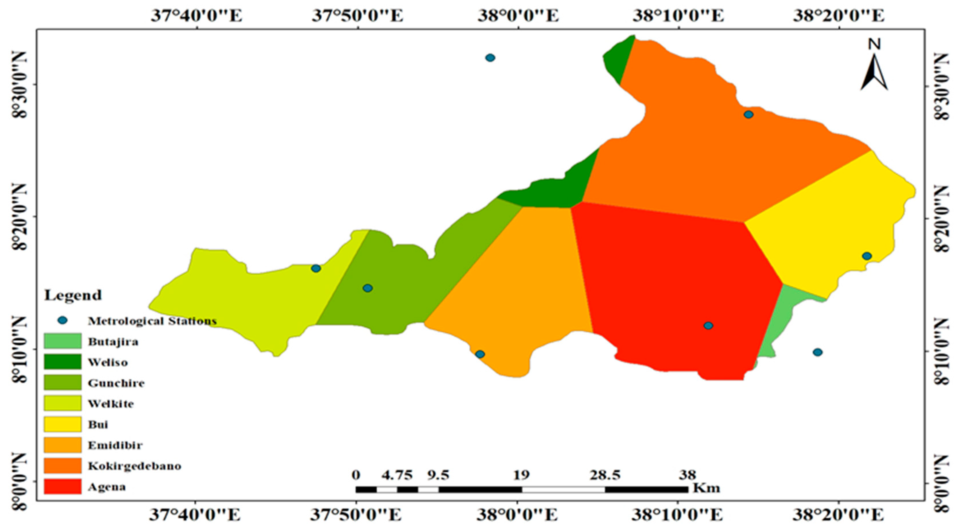
2.1. Description of the Study Area

The Wabe watershed, originating in the northeastern region, is recognized as one of the primary tributaries within the expansive Omo River basin. The Wabe River originates from the Guraghe mountain range and then joins the Gibe River within a sub-catchment of the Omo basin. The area under consideration is within the Guraghe zone, situated in Central Ethiopia, at an estimated distance of 160 km from Addis Ababa, the country’s capital city. The Wabe River catchment lies situated between 07°50′0′′ and 08°40′0′′ N and 37°40′0′′ and 38°20′0′′ E (Figure 1), with elevations ranging from 1014 to 3611 m above sea level and a drainage area of about 1840 km2.The study area is accessible through an asphaltic road from Addis Ababa to Welkite and then through a weathered gravel road to the catchment. Several interconnected all-weather roads could render good access within the catchment.

2.2. Physiography

Gentle slopes, undulating terrain, and steep slopes distinguish the research region. The study area’s northeast, east, and southeast corners frequently have elevated topography, while the middle and southwest lowland regions typically have very flat to gently sloping terrain. At the mouth of the Wabe catchment, the height is below 1094 m, and the maximum elevation is about 3601 m to the northeast (Figure 2). The Wabe River basin has an average height of 2347 m. It is flanked by highlands along the Guraghe range in the northeast, lowland lowlands in the catchment’s southwest, and a transitional region that stretches from the southeast corner of Woliso in the north to the Agena area in the south. In general, spatter cones, escarpments, and ridges dominate the geomorphology of the catchment.

2.3. Climate

Ethiopia offers many climates, from scorching plains to frigid mountains. In the Dalol depression, the altitude ranges from around 120 m below sea level to 4620 m above sea level in the Semien Mountains highlands. This climate system is typically categorized depending on the temperature and altitudinal range. As a result, the nation is divided into five climate zones. The Kola zone can be characterized as a warm and arid area situated at an elevation ranging from 500 m to 1500 m above sea level. However, it should be noted that the Berha zone is characterized by high temperatures and extreme aridity, making it a challenging environment. The altitude in this region does not exceed 500 m above sea level [27].
The ideal temperature range for Woina Dega is shown to occur at elevations ranging from 1500 m to 2500 m above sea level. The Dega and Wurch regions are typically located in elevated areas, with heights ranging from 2500 to 3000 m and over 3000 m above sea level, respectively [27]. The Indian and Atlantic Ocean monsoons considerably influence the geographical and temporal variation of the Ethiopian climate system, which is strongly regulated by the inter-annual movement of the position of the Inter Tropical Convergence Zone [28]. According to Armanuos et al. [28], the Wabe River catchment was located in a climatic zone between Wurch and Woina Dega. On the rift floor, the subtropical Woina Dega climate dominates, while the escarpment and nearby highlands are home to temperate, humid Dega zones. The catchment has a mean minimum temperature of 9 °C and a mean maximum temperature of 25 °C, with an elevation range of 1094 to 3601 m above sea level and temperature variations with altitude. The average annual rainfall in the region is 1374.26 mm/year.

2.4. Slope

The slope map for the designated research area was generated by employing the spatial analysis tool inside the slope module of ArcGIS 10.8 in conjunction with a digital elevation model (DEM). The slope map of the Wabe catchment (Figure 3) illustrates that the slopes within the study region exhibit a range of slopes and are divided into six categories: 0–4% (very gentle), 5–8% (gentile), 9–13% (moderate), 14–20% (moderately steep), 21–31% steep, and greater than >31% is a very steep slope (Figure 3). Areas with a slope of 0 to 7 degrees typically suggest flat or plain terrain, which is excellent for surface water settling and infiltration. Consequently, this location may have groundwater potential.

2.5. Methodology

To achieve the objectives of the present study, the approach used to estimate the groundwater recharge for the Wabe watershed passes through three steps. The first stage included a review of the literature and gathering existing data. Data sources included published and unpublished reports from different sources. The fieldwork in the second stage entails examining the research area’s topography, soil type, land use/cover, geology, hydrogeology, and drainage system. Soil, land use/cover, and geological and hydrogeological maps were amended based on field observations. Topographical, hydrological, hydrogeological, geological, meteorological, and soil information was compiled for recharge modelling. GIS and remote sensing are crucial for manipulating, storing, and analyzing digital data. The files above necessitate modification and preparation to conform to the requirements of raster grid cells. Delineating a watershed was carried out with the digital elevation model (DEM) obtained from the Shuttle Radar Topography Mission (SRTM). The software ArcGIS 10.8, together with its spatial extension, was employed to perform further processing of the digital elevation model (DEM) and delineate the basins. A land use/cover map of the study’s region was created using ArcGIS 10.8 software, data obtained from the WLRC (Water and Land Resource Centre), and GPS field data. ArcGIS 10.8 was utilized to generate weather information, groundwater level data, land use/land cover (LULC) data, reclassified soil maps, elevation maps, and slope maps.
The WetSpass-M model typically necessitates two distinct types of inputs for its execution: a grid map in ASCII file format and parameter tables in TBL file format. The model additionally requires data from the parameter table about land use, soil characteristics, and the frequency of wet days. The input parameters were generated using ArcGIS (version 10.8) and its inverse distance weight spatial analyst extension. Data interpolation was performed to construct these parameters for input, and parameter tables were provided as attributes to the maps. As model inputs, grid maps for potential evapotranspiration, topography, slope, groundwater level (groundwater depth), soil, and land use/cover were also constructed. Because of this, the slope map and topographic/elevation grid map were created using ArcGIS 10.8 with SRTM DEM 30 × 30 m resolution.
Subsequently, the entire set of raster data underwent a conversion process to the ASCII format. The WetSpass-M model relies on ASCII-structured raster data to provide accurate maps of ET, total runoff, and yearly and seasonal recharge within the designated research area. While the WetSpass-M model was running, the value of a single (target variable) parameter was raised by varying percentages by maintaining the values of other parameters. The procedure was typically followed for other parameters in the same way. Before understanding the model’s findings, the sensitivity of the input parameter was measured, and the model outcomes were calibrated to determine whether the outcome was acceptable.
Additionally, the observed values for stream discharge and the simulated model result of surface runoff were correlated. The present study has utilized groundwater recharge data from the Wabe catchment to analyze the geographical variability of water balance components over an extended period. This analysis used a physical-based quasi-steady phase time-independent model known as WetSpass-M.

2.5.1. Data Collection and Analysis

Relevant data or information must be present for this research project to be reliable. This information includes meteorological (rainfall, temperature, potential ET, wind speed, relative humidity, and sunlight hour) and hydrological (streamflow) data. The WetSpass-M model utilized physical data about the area to evaluate groundwater recharge within the watershed. This included land use/cover information, soil texture, and slope.

2.5.2. Estimation of Missing Data

One of the primary objectives of conducting hydrological and meteorological investigations is to obtain reliable and credible data. In meteorological data, missing data are a regular issue. However, data on precipitation is frequently unreliable. According to [28], the lack of completeness in precipitation data may result from deteriorated measuring equipment, measuring errors, geographic data scarcity, changes in measuring sites or data collectors, irregular measurement practices, or significant recent changes in the region’s climate.
Various meteorological data were gathered and reviewed for any missing information. Several techniques have been put forth to approximate missing rainfall data. This study calculated a weighted mean of the average annual rainfall at each station using the normal ratio and station average methods. The accuracy of the station average technique may be compromised if there is a deviation of more than 10% between the annual rainfall at any of the n stations and the annual rainfall at the specific location of interest. The normal ratio approach is preferred if the condition mentioned above exists [31,32,33]. Equation (1) shows the %difference calculation.
% difference = N x N i N x × 100
where Ni is the annual rainfall at the site of interest and Nx is the total yearly rainfall across all areas.
If the mean difference is greater than 10%, the normal ratio method should be used using the following Equation (2).
P x = N x M P 1 N 1 + P 2   N 2   + + P m N m        
where Nx = mean annual rainfall at the missing data. N1, N2, N3, and Nm = average yearly precipitation in mm at the adjacent site.

2.5.3. Meteorological and Hydrological Data

The utilization of long-term hydrological and meteorological data obtained from reputable sources such as the National Meteorological Agency (NMA) and Ethiopia’s Ministry of Water and Energy (MoWE) (Addis Ababa, Ethiopia) plays a crucial role in calculating water balance and assessing groundwater recharge. From the Ethiopian National Meteorological Agency (ENMA), various types of meteorological data relevant to this study have been collected. Measurements of precipitation, air temperature, wind speed, relative humidity, and sunshine length are taken every three hours at the principal station, also known as a class one station, according to the agency’s classification. Class three (or ordinary) stations are another group of locations where daily observations of precipitation and air temperature are made.
Additionally, Class Four stations only provide daily precipitation measurements. According to this classification, Bui and Emdibir stations are the principal ones. In contrast, the others are class three stations that just record temperature and precipitation, and class two stations are not present in the present study area. Table 1 shows the location, elevation, and class type of the meteorological stations surrounding the study area. The station was chosen based on its long-term data availability, its influence on the research region, stations nearby with representative coverage that were also chosen, and class. The period from 1991 to 2021 is chosen to analyze meteorological data, specifically precipitation, evapotranspiration, temperature, and wind speed. The mean values for each seasonal time step, namely winter (October to May) and summer (June to September), are considered. The meteorological data that was accessible was utilized to generate annual and seasonal weather attributes. There are a total of eight meteorological stations situated either inside or close to the Wabe catchment area. All stations collect monthly data on precipitation and temperature. However, only two stations gather relative humidity, sunlight hours, and wind speed information. The annual average precipitation was calculated by utilizing the mean monthly precipitation data obtained from both the wet and dry seasons, which encompass the months of June to September and October to May, respectively.
The data received from the eight stations were utilized to generate digital maps of precipitation patterns by applying the inverse distance weight (IDW) interpolation module in ArcGIS. Spatial analysis offers several interpolation algorithms for raster data, such as IDW, spline, and kriging. Each of the above methods was employed to generate a surface representing the mean climatological information for the catchment area. The mean of the monthly climate variables and hydrologic model input raster location maps for 1991–2021 were generated using the IDW interpolation method within the spatial analyst tool of a Geographic Information System (GIS) system. The IDW interpolation technique is preferred over alternative methods because of its ability to assign greater significance to adjacent values compared to more distant ones.
Furthermore, the strategy exhibited higher accuracy in terms of mean square error compared to alternative approaches [33]. When the rainfall and temperature in the research region are known, the potential evapotranspiration (PET) may be calculated and understood. There are various techniques for estimating PET. However, the approaches differ according to the climatic factors needed for calculation. The PET for eight meteorological stations in the Wabe watershed was estimated using the Thornthwaite method [34,35] due to a lack of PET data. A number of studies have been conducted on the application and improvement of the Thornthwaite method. According to Trajkovic et al. [36], local coefficients are used to correct Thornthwaite PET, thereby supporting temperature-based estimates of reference PET and aridity indices [37]. PET model evaluation, modelling, and projection under climate scenarios were studied in the Kesem sub-basin, Awash River basin, Ethiopia [38].

2.6. Methods of Recharge Estimation

WetSpass-M Modeling

Hydrometeorology has grown as a professional discipline of hydrology connected to the basic information of meteorology and the desires of the hydrologist. The hydrologist will usually be able to request the facilities of a professional meteorologist for weather forecasting and special studies to emphasize the depth of precipitation for the assessment of available water resources, daily temperature, and evaporation conditions in an area. Most importantly, an overall understanding of precipitation and evaporation is essential if the hydrologist is to appreciate the complexities of the nature of the atmosphere [39]. It is the primary focus of meteorologists to understand the overall atmospheric circulation to predict the trajectory of pressure systems and the accompanying wind patterns and weather conditions in a particular region [40].
WetSpass-M is an acronym derived from the phrase “Water and Energy Transfer between Soil, Plants, and Atmosphere under quasi-steady phase,” as introduced by [22]. The term “M” is an abbreviation used to refer to a monthly simulation. WetSpass was developed by [22] to estimate the scattered elements of the water balance on a yearly scale over the long term. The WetSpass-M model is a downscaled version of the original WetSpass model, designed to operate at a monthly temporal resolution. The model incorporates many input datasets, such as gridded maps based on long-term net weather information, land use/cover, water level, slope, digital elevation model (DEM), and soil map, to replicate typical spatial and temporal water balance patterns [22]. The calculation of monthly evapotranspiration involves the summation of three components: the evaporation of water intercepted by plants, the transpiration of the vegetative cover, and the evaporation occurring from the exposed soil surface without vegetation. The remaining water balance is composed of groundwater recharge, which is determined by deducting precipitation from the combined values of surface runoff and actual evapotranspiration.
The water balance element is executed at the raster cell level due to the scattered nature of the model. Based on this methodology, the comprehensive water equilibrium of every raster cell is partitioned into distinct water equilibriums for its impermeable, planted, bare-soil, and open-water segments. This enables the consideration of the heterogeneity of land use inside each cell, which is contingent upon the resolution of the raster cell. The computation of the water balance in the research region involves aggregating the water balance calculations for individual cells in a specific sequence, namely surface runoff, real evapotranspiration, and groundwater recharge.
Different factors, such as climate variability, soil types, land use/cover or vegetation, topography or altitude, and geology, may affect groundwater recharge in the catchment. The climate affects the hydrological system parameters, particularly the local area’s time- and space-based rainfall distribution. Variations in soil type, vegetation cover, topography, and geology influence an area’s sources and sinks, and consequently, its capacity to hold water affects recharge. Estimating groundwater recharge is a significant challenge in the management of groundwater resources. Meteorological factors influence the hydrological cycle, including precipitation, weather patterns, soil characteristics, soil moisture levels, vegetation density, slope conditions, agricultural techniques, and evapotranspiration [23]. The WetSpass-M model is used to determine the long-term distribution quantities of groundwater recharge in the Wabe catchment. As a result, surface runoff, interception, and actual evapotranspiration are deducted from the corresponding seasonal and yearly precipitation values. WetSpass estimates seasonal and annual groundwater recharge quantities within the Wabe basin over an extended period.
The determination of surface runoff is accomplished by utilizing the WetSpass-M model, which involves a two-step process. During the initial phase, the potential surface runoff (Sv-pot) estimation is derived by multiplying a coefficient with the difference between precipitation and interception. The calculation of surface runoff was performed utilizing Equation (3).
S v p o t = C s v P I
The study conducted by [41] suggested that factors such as soil type, slope, and vegetation influence the surface runoff coefficient (Csv) in places with vegetated infiltration. Surface runoff, or Sv, is observed in areas where groundwater discharge zones are saturated. The value of the coefficient for surface runoff in this region is significantly elevated, and it is believed to remain constant due to its dependence on the slope rather than soil composition, vegetation coverage, or proximity to the river. The second phase involves calculating actual surface runoff using potential surface runoff (Sv-pot), which considers the variations in precipitation intensities and soil penetration rates. Horton’s infiltration Equation (4) is only accurate when total rainfall intensity surpasses infiltration. CHor is a seasonal precipitation coefficient that impacts Hortonian overland flow (HOF) or surface runoff.
Sv = CHor Svpot
The coefficient CHor is utilized to parameterize seasonal precipitation, which plays a role in the generation of surface runoff or Hortonian overland flow (HOF). The various levels of precipitation intensity within groundwater discharge areas impact the process of surface runoff. Hence, it may be concluded that CHor is equal to 1.0 because all intensities of rainfall have an impact on the generation of surface runoff. Surface runoff in recharging zones can only be generated by storms characterized by substantial wind velocities.
The WetSpass-M GIS-based model determines total actual evapotranspiration (AET), water transpiration from vegetative cover, water intercepted by vegetation, and evaporation from the bare soil between the plants. The WetSpass-M model, which is one of the components of the water balance equation [22], may determine AET. A vegetation coefficient must be computed to calculate the reference transpiration from PET. Equation (5) is used to calculate the vegetation coefficient.
c = 1 + γ 1 + γ 1 + r c   r a
where c is the vegetation coefficient and used to calculate the transpiration component of the water balance, γ is the psychometric constant [ML−1T−2C−1], Δ is the constant proportionality slope of the first derivative of the saturated vapour pressure curve (slope of saturation vapour pressure at the prevailing air temperature) [ML−1T−2C−1], canopy resistance is represented by rc in the unit [TL−1], and aerodynamic resistance is denoted by ra in the unit [TL−1] given in Equation (6):
r a = 1 K 2 U a z a l n Z a Z d Z o 2      
where K is the von Karman constant (0.41), 𝑈𝑎 (m/s) is the wind speed at elevation 𝑍𝑎 (m), 𝑍𝑑 is zero displacement elevation (m), and 𝑍o is the surface aerodynamic roughness height (m). The vegetation coefficient is equal to one for vegetated area discharge of groundwater. Therefore, the reference transpiration (𝑇𝑟𝑣) is given in Equation (7):
Trv = cEoTp
where Trv represents the reference transpiration of a vegetated surface [LT−1], EoTp represents the potential evaporation of open water [LT−1], and c represents the vegetation coefficient. The vegetation coefficient can be determined using the reference vegetation transpiration ratio. The total actual monthly ET per grid cell [ETraster (mm/month)] can be calculated using Equation (8):
ETraster = avETv + asEs + aoEo + aiEi
where ETraster is the total evapotranspiration at the raster cell; av, as, ao, and ai are area components of vegetated, bare-soil, open-water, and impervious segments [22].
The primary objective behind developing the WetSpass-M model aimed to calculate the average yearly spatial distribution of water balance elements, including groundwater recharge, as outlined by [22]. The WetSpass-M model utilizes Equation (9) to compute the water balance and simulate monthly and annual groundwater recharge.
P = I + Sv + ETv + Gwr
where 𝑃 is the mean annual precipitation [LT−1], I is the interception of rainfall by vegetation [LT−1], Sv is surface overland flow [LT−1], ETv is the actual transpiration vegetation cover [LT−1], and Gwr is recharge amount of groundwater [LT−1]. The WetSpass model’s final output is the spatially distributed groundwater recharge estimation. This value can be determined by applying Equation (10) to the water balance:
Gwr = P − Sv − Etv − I
where P represents mean annual precipitation, Sv represents surface overland flow, Gwr represents the total amount of groundwater recharge, I indicates interception by vegetation, and ETv represents the actual evapotranspiration [LT−1] calculated as the sum of transpiration Tv, and Es means the evaporation from bare soil found in between the vegetation As a result, groundwater recharge depends on precipitation, temperature, land use/cover, soil type, slope, topography (elevation), groundwater level, and other input factors utilized in the WetSpass model.
The water balance calculations for a particular basin are carried out at the individual raster cell level to evaluate long-term trends. The model employs long-term average hydro-meteorological and biophysical aspects as input variables to simulate spatial-temporal water balance components, such as groundwater recharge, surface runoff, and real ET. The calculation of the comprehensive water balance for every raster cell and season may now be achieved by employing the water balance components for vegetated, bare-soil, open-water, and impermeable sections of a raster cell, as outlined in Equations (11)–(13) [22].
        E T r a s t e r = a v E T v + a s E s + a o E o + a i E i
S r a s t e r = a v S v + a s S s + a o S o + a i S i
R r a s t e r = a v R v + a s R s + a o R o + a i R i
ETraster, Sraster, and Rraster denote evapotranspiration, surface runoff, and recharge. Subscripts refer to the raster cell’s vegetation (v), bare-soil (s), open-water (o), and impervious areas (i), whereas av, as, ao, and ai are the fractions of each land cover in a raster cell.

3. Results and Discussions

3.1. Hydro-Meteorological Data Analysis

Each hydro-meteorological component must be quantified to evaluate the water balance of the watershed. Hydro-meteorological data, including precipitation, temperature, wind speed, and PET, are crucial in understanding atmospheric events and estimating the recharge of catchment areas. Interpolating data obtained from meteorological stations was used to estimate the variables of rainfall, evaporation, temperature, and wind speed during the simulation process. Using the inverse distance weight approach, this interpolation was performed. Therefore, assessments of real ET, surface runoff, and groundwater recharge have been conducted and will be discussed in further detail in the following sections.

3.1.1. Rainfall

The National Meteorological Agency’s Hawasa branch provided the long-term weather data. Daily rainfall data with the reference years (1991–2021) for eight long-term records of rainfall stations located around or inside the catchment are used to compute rainfall’s spatial and temporal variation. These data generated the Wabe catchment’s summer, winter, and mean annual rainfall distributions.
The Thiessen polygon method seeks to account for non-uniform gauge distribution by weighing each gauge record in proportion to the region closest to that gauge compared to any other gauge. The polygons were constructed using ArcGIS computer code, and the impact areas for the eight stations were obtained (Figure 4). The precipitations of each polygon were determined by multiplying the area weighing percentage by the point precipitation encompassed in the polygon (Table 2).
Rainfall patterns in the study area are mono-modal, with peaks in July and August. Generally, the rainy season lasts from June to September, with the dry season lasting from October to April. April and May are transitional months with light precipitation. Precipitation variation occurs spatially throughout the catchment. There are high variations between highlands and lowlands due to significant elevation variations. Even though altitude is a determinant factor for precipitation, Kokirgedebano station has a high rainfall compared to other stations except for Bui and Butajira. This incremental precipitation may be about Gurage Ridge because the station was close to the mountain. The other stations go ahead with the principle of rainfall—the altitude relationship—the trend of the spatial distribution of precipitation. The area receives minimum, maximum, and mean annual rainfall of about 1087 mm, 1767 mm, and 1374.26 mm, respectively, and the average summer precipitation is 855.2 mm, whereas the winter is 515.5 mm. Figure 5 shows the seasonal and annual average rainfall map of the Wabe catchment.

3.1.2. Temperature

Temperature controls how quickly water molecules evaporate from a surface and move into the air above. It affects the rate of evaporation temporarily. Temperature records are accessible for all meteorological stations in the research area. It fluctuates spatially and gets bigger while generally getting smaller as you ascend altitude. The arithmetic average of the mean daily temperatures for all days is used to calculate the mean monthly temperature. It is measured at eight locations. In the winter (dry) season, the average temperature ranges from 17.24 °C to 21.06 °C with a mean of 18.47 °C; in the summer (rainy) season, the average temperature ranges from 16.20 °C to 19.79 °C with a mean of 17.48 °C; and the annual intermediate runs from 16.81 °C to 20.65 °C with a mean of 18.11 °C.

3.1.3. Potential Evapotranspiration (PET)

Water loss to the atmosphere through evaporation from all surfaces, including soil, plants, and free water surfaces, is known as PET. Solar radiation, temperature, wind speed, atmospheric pressure, water vapour in the air, and moisture availability at the evaporating surface all affect PET. It would happen if a wholly vegetated surface always had access to an appropriate water supply. According to Thorntwait and Mather [31], the amount of water would have evaporated if the soil had an endless supply of water to evaporate. Essentially, climatic factors control PET. It rises with rising temperatures, sunshine, wind speed, and falling humidity. There are various formulae for determining PET, but Thornthwaite methods are used based on the given data in this study.
The monthly PET data were categorized into two hydrological seasons: the eight-month winter (dry season) and the four-month summer (wet season). The inverse distance weight spatial interpolation approach was employed for both hydrological seasons to obtain the distribution value for the catchment’s PET. The WetSpass-M model uses these spatially distributed PETgrid maps, translated into ASCII format using the ArcGIS conversion tool, as input parameters to calculate AET and other water balance components. The winter mean PET is 560.8 mm, while the summer average is 267.2 mm. Average evapotranspiration for the year is 828.6 mm, with the lowest and highest readings being 779.4 mm and 921.6 mm, respectively (Figure 6).

3.1.4. Wind Speed

Wind speed has a vital role in controlling the rate of evapotranspiration. It has a direct relationship to evaporation. According to [41], as water vaporizes into the atmosphere, the layer between the earth and the air becomes increasingly saturated, requiring the water vapour to be continuously evacuated and replaced with drier air. More rain falls on the windward side than the leeward side when moisture-laden air is pushed to rise over a mountain barrier. There are only a few meteorological stations with data on wind speed. These data were applied consistently across the area. The observations on wind speed are also categorized into two distinct seasons: four months during the summer (June to September) and eight months during the winter (October to May). An inverse distance weight interpolation method was used for each season’s average wind speed statistics. The two wind speed grid maps were converted into ASCII files and used as input variables for the WetSpass-M model. During the summer and winter seasons, the mean wind speed is 0.87 m/s and 1.60 m/s, respectively, with the yearly mean being 1.32 m/s (Figure 7).

3.1.5. Groundwater Depth

WetSpass relies on the groundwater level map for estimating groundwater recharge. To assess site accessibility, groundwater depth, also known as static water level, was measured during the construction of the water well. An observation pipe with a dip meter was used for this measurement. The data were interpolated using the ArcGIS IDW spatial analyst function to depict the catchment area accurately. The shallow groundwater level in topographically low-elevation locations results from the fact that most unconfined aquifer water tables generally follow topography. Hence, to produce the groundwater level map of the Wabe River catchment, 14 water points and their respective static water levels have been used. The static water level in the Wabe catchment ranges from 21.3 to 129.3 m below the surface, indicating low-elevation areas of the catchment.
The water levels collected from shallow and deep wells in the catchment were used to compute the groundwater level and the ground elevations of the well location. The equilibrium between recharge and outflow often regulates the groundwater levels in these wells. It is common to find water levels below the surface of the earth. Sometimes, though, the water level is seen to be higher than the surface of the land. The phrase “intermediate zone” refers to the regions between recharge and groundwater discharge points. Discharges can happen in the pumping of wells, rivers, lakes, and other bodies of surface water in addition to the atmosphere. It indicates an increase in water levels in the eastern and southeast portions of the watershed, from Welkite–Gubre towns to Mehalanba–Hawariyat–Agena towns. The area with the highest water levels was Kechen Kebele in the Muhur Aklil district, where this pattern is still evident. The water level contour indicates a general fall from the southern part of Guraghe ridge to the confluence point of the Wabe and Omo-Gibe rivers, which is in keeping with the topography variance of the watershed.
Two groundwater flow directions were identified in the study area. The first one is from Tawula–Welkite in the west to the Weliso areas in the north, suggesting that this region is one of the basin’s recharge sources. The second is the principal flow direction, which is anticipated to move from the Guraghe and southeast ridges of the watershed to the northwest and western regions. In addition to the high-discharge springs, high-discharge boreholes have lately been drilled relatively close to these water source locations (southeastern). These are the primary water sources for the people living in these catchment areas. They are also utilized for irrigation in some areas of the catchment. This means that the Guraghe Ridge is one of the catchment’s primary water sources. Figure 8 shows the groundwater level map of the study area.

3.2. Output of WetSpass-M Model

WetSpass-M provides a comprehensive representation of the Wabe watershed. Due to its complete expression and distribution of the catchment’s hydrological, physical, and meteorological characteristics, the model can identify geographical and temporal variations in the water balance components of the catchment. ASCII files contain the model’s monthly simulated outcomes, including actual evapotranspiration (AET), surface runoff, and recharge. Following the objectives of this study, these results can be used to derive the desired seasonal and annual values. A seasonal result denotes the climate condition of the catchment, which is wet (June to September) and dry (Oct to May) seasons. The output water balance component of WetSpass is briefly described as follows.

3.2.1. Actual Evapotranspiration (AET)

A variety of input parameters and variables are used to simulate the water balance component of the model using the WetSpass-M model. Water balance assessments at the watershed level are critical in arid and semi-arid environments where actual evapotranspiration (AET) is measured [18]. Alternative methods are commonly used to estimate actual evapotranspiration due to the challenges and limitations of quantifying it. Hydrologic models, empirical formulas, and potential evapotranspiration are some of the methods.
AET was simulated for the Wabe catchment on an annual and seasonal basis. The quantity of precipitation lost owing to interception varies with vegetation species, age, planting density, and time of year. The amount of water that its botanical classification primarily determines a plant intercepts. There are two possible fates for water trapped on the surface of a leaf: it can either descend to the ground or evaporate. The interception fraction represents a certain percentage of the total annual precipitation depending on the vegetation type—the annual precipitation ranges from 31.63 mm to 337.89 mm, with an average of 202.42 mm. According to the readings, the lower and upper bounds are 515 mm and 775 mm, respectively, while the mean annual evaporation from exposed soil amidst vegetation is approximately 665 mm.
According to the WetSpass-M model, the catchment’s mean annual evapotranspiration (ETv) is 701.11 mm. The lowest ETv value recorded is 541.1 mm, while the highest ETv value recorded is 804 mm. In a given catchment area, actual evapotranspiration represents around 51% of the total precipitation. The mean ETv of the catchment is 278.1 mm with a standard deviation of 14.72 during the rainy season, while the mean and standard deviation values are approximately 423 mm and 50.32 during the dry season, with minimum and maximum values of 245 mm and 309 mm, respectively. Figure 9 shows the seasonal and annual actual evapotranspiration maps of the Wabe catchment. This happened due to changes in precipitation and other factors between the two seasons, and the winter evapotranspiration is larger than the summer. Several factors have contributed to the observed change, including a reduction in cloud cover, a decrease in relative humidity, and a lengthier winter than a summer season.
Regarding spatial distribution, due to the presence of cultivated crops, woodland, and significant yearly rainfall in the northern, middle, and southwestern portions of the catchment, there is a high annual actual evapotranspiration in these regions [8,16]. However, due to the sparse coverage of forests and woodlands and the low yearly rainfall, the catchment’s southern and southeast regions exhibit lower annual evapotranspiration. In general, land use/cover and precipitation influence the annual evapotranspiration value of the Wabe watershed [10,23]. Land use/cover and precipitation play a significant role in determining evapotranspiration in the catchment.

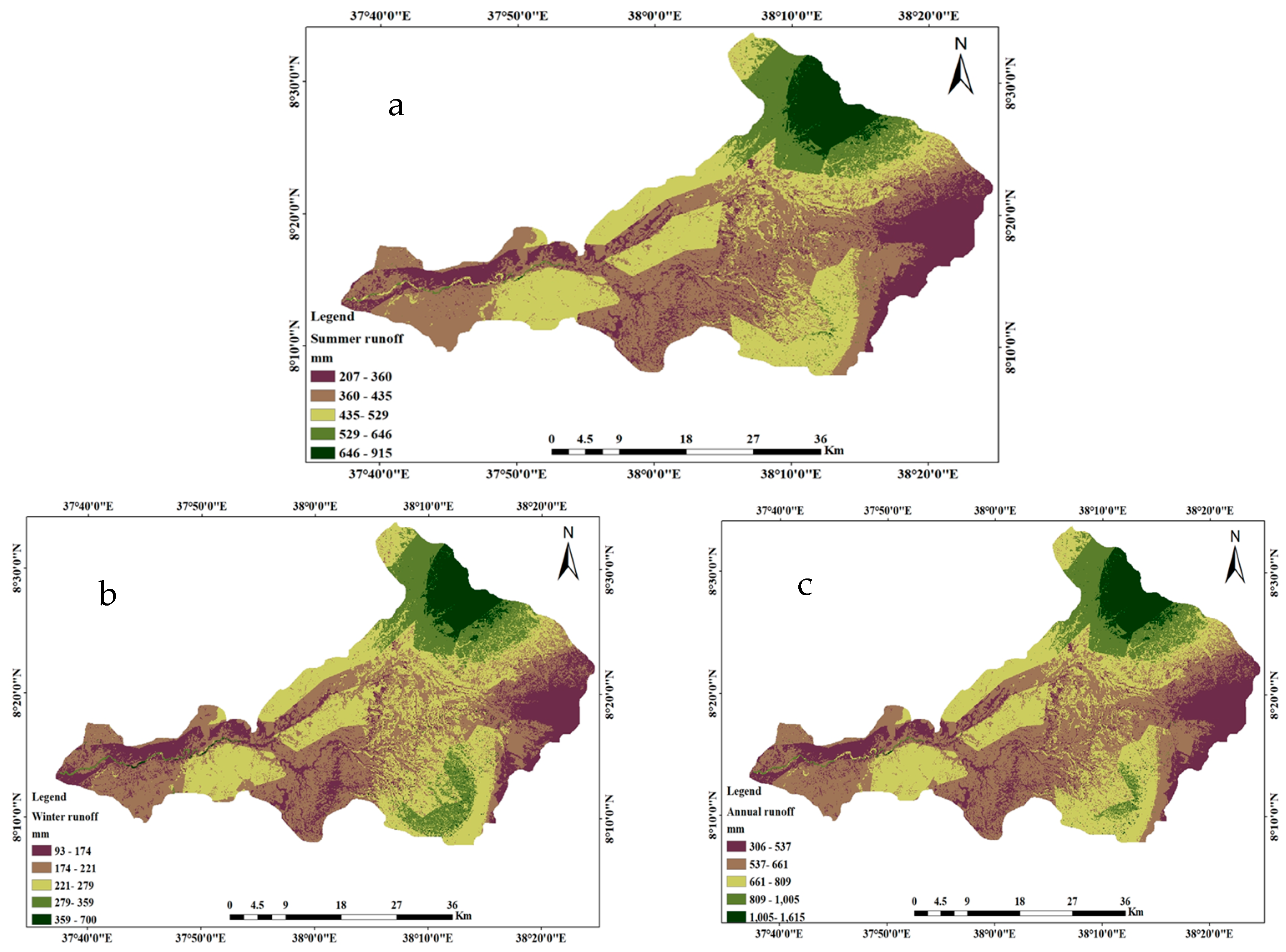
3.2.2. Surface Runoff (Qo)

Several inputs and parameters are used in the WetSpass-M model to determine the monthly surface runoff (SV). Various factors influence hydrological processes, including vegetation type, soil texture, slope, and meteorological factors [22]. Several input variables within the Wabe watershed significantly impact the quantity of runoff. An average yearly surface runoff (Qo) was simulated using the WetSpass-M model. There are fluctuations in the variability of surface runoff during both the summer and winter months.
The minimum, maximum, and mean of the WetSpass-M model estimated annual surface runoffs for the Wabe catchment to be 306 mm, 1615 mm, and 468.64 mm, respectively. In the rainy season, the catchment’s mean surface runoff (Sv) is 358.9 mm with a standard deviation of 99.19; in contrast, the mean and standard deviation of Sv during the dry season are 231.4 mm and 65.81 mm. Figure 10 shows the seasonal and annual surface runoff maps of the Wabe catchment. The average value of the Wabe catchment area represents 34.1% of the cumulative yearly rainfall. Variations in precipitation patterns between the two seasons can explain the observed variances. Precipitation levels are higher during the rainy season, which extends from June to September, compared to the dry season, which lasts from October to May. Thus, there is more runoff in the summer than in the winter. Due to the presence of cliff terrain, steep slopes, clay soil, and little vegetation cover in the catchment area’s northern, central, and southwestern regions, surface runoff has been elevated. Water percolation into the soil and replenishment of groundwater are increased by vegetation, improving rainfall receipt and ET. Most of the Wabe catchment’s northwestern, eastern, and southern regions have minimal surface runoff because of woodland, grassland with shrubs and high vegetative cover, farmland, loam, sandy loam, and a mild slope. Landscape land use/cover significantly impacts the Wabe catchment’s surface runoff.

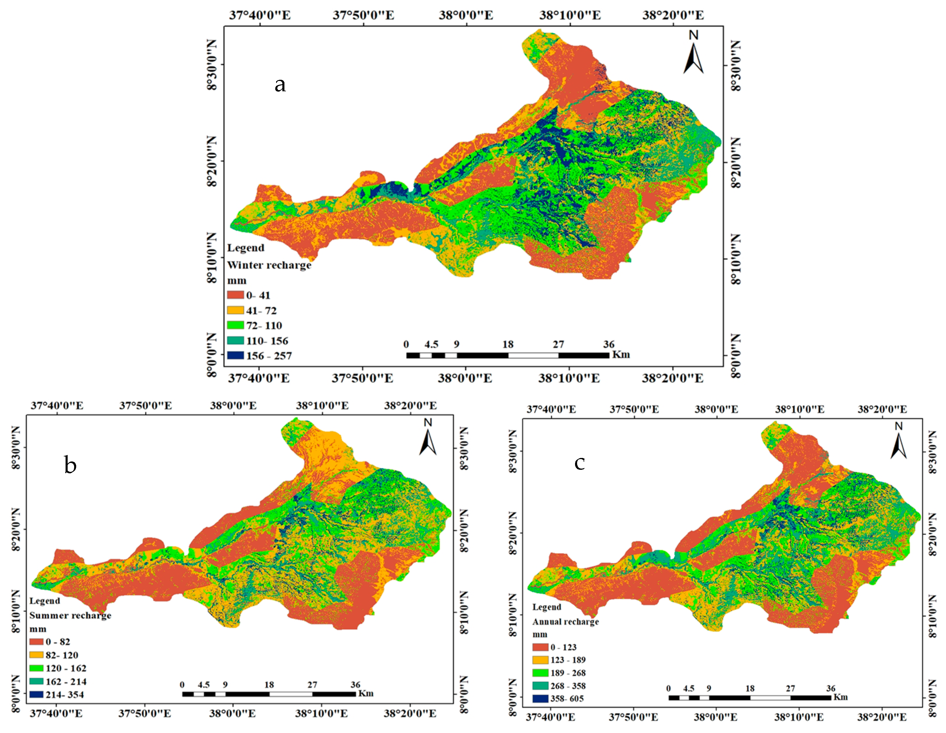
3.2.3. Groundwater Recharge

Based on simulations conducted using the WetSpass-M model, the Wabe watershed exhibits a 0 mm to 605 mm range for long-term minimum and maximum groundwater recharge values. The average groundwater recharge in this catchment is 204.51 mm, corresponding to approximately 14.8% of the total annual precipitation. According to the model, the quantity of seasonal recharge varies between the summer and winter seasons. During the summer months (June to September), the catchment’s groundwater recharge varies between 0 and 354 mm, with an average value of 125.53 mm. Approximately 85% of this recharge is derived from the catchment’s yearly recharge. Based on the data presented in Figure 11, the winter recharge ranges from 0 to 257 mm, with an average of 78.98 mm. Approximately 15% of the total recharge is accounted for by this value. Figure 11 shows seasonal and annual groundwater recharge maps (a. summer, b. winter, and c. annual) of the Wabe catchment.
The recharge amount varies spatially, with a significantly greater recharge value in the middle and northern regions of the catchment during both seasons. The catchment’s mean annual groundwater recharge is 345,128,800 m3/year. The rate at which groundwater percolates is influenced by several factors, including vegetation cover, slope of the land, soil type, water table level, and the presence or absence of limiting beds.
Recharge zones typically exhibit more conspicuous topographic features than discharge zones. Depending on the region’s topography, it may not be possible to delineate the recharge and discharge zones of the area. Several factors influence the division of an area into recharge and discharge zones, including land use and cover, soil types, and terrain features. Compared to the lowlands, the highlands experience a significantly higher level of precipitation. Geological formation and the structural density of a region can influence the rate and volume of groundwater recharge. Alluvium and extensively weathered rhyolite are the dominant geological formations in the upper section of the study region. On the other hand, the lower part of the catchment and the Nazret formation receive less groundwater recharge.
The map in Figure 10 demonstrates how the northern and northwestern regions have high groundwater recharge rates because of the sandy loam soil type, thick forest, vegetation, and heavy rainfall. In the eastern and southeastern areas of the research region, groundwater recharge rates are also high. These factors include ploughed soil, cultivated crops, irrigated areas, mild to moderate slopes, and low drainage density. Despite this, the southern and southwestern regions experience limited groundwater recharge due to high drainage density, steep topography, impermeable clay soil, and little ground cover. Wabe catchment typically exhibits significant evapotranspiration and surface runoff, but seasonal and annual recharge amounts are quite low.

3.2.4. Monthly Simulated Groundwater Recharge Raster Maps

The WetSpass-M model was used for monthly water balance simulation based on long-term average monthly data [23,24]. This study used long-term monthly average rainfall, PET, temperature, and wind speed with the previously used raster maps of elevation, LULC, slope, and soil and simulated monthly groundwater recharge maps. The following maps show the distribution of recharge within different months. Therefore, the months of high recharge are identified using the mean value of each month. Months of lower groundwater recharge are December (3.85 mm), November (3.8 mm), January (4.54 mm), and February (4.4 mm), whereas the months with high groundwater recharge are July (32.3 mm), August (43.6 mm), and September (32 mm). The months with the maximum recharge are July (32.3 mm) and August (43.6 mm).

3.3. Model Verification

According to previous research, evapotranspiration is primarily affected by rainfall and a particular area’s land use/land cover characteristics. According to Arefaine et al. [20], areas with high evapotranspiration rates and water amounts are spatially correlated. A moderate slope and dense vegetation were also associated with low surface runoff values. Surface runoff is greater during the summer than in the winter [31]. As a result of land degradation and soil erosion, the Wabe watershed faces significant environmental challenges.
There was no groundwater recharge on open water bodies since groundwater fell onto the lake’s surface [26]. According to [42], the average groundwater recharge rate for all local water bodies is low, suggesting high discharge and low recharge rates for these water bodies. The recharge of groundwater was strongly correlated with locations with moderate to highly gentle slopes. There is an association between gentle slope locations and high groundwater recharge.
There is a correlation between groundwater recharge and places characterized by gentle vegetation and a landscape with a medium soil texture, as indicated by [29]. Many factors contribute to recharge promotion, including a flat topography, a deep-water table, natural vegetation cover, and the absence of limiting beds [43]. Ref. [3] found a positive correlation between dense vegetation and high interception values in spatial distributions. As a result, the results of this study were compared with those of previous research. The researchers have integrated WetSpass models with GIS and remote sensing techniques. The primary components of the spatial arrangement of the water balance were evaluated comprehensively. Groundwater recharge was limited in the basin due to high runoff levels and evapotranspiration.
Scholars studied the water balance components of different watersheds with similar geological and climatic conditions to those of the present study area [24,27]. Ref. [24] reported 59.76% of evapotranspiration, 20.6% of surface runoff, and 19.65% of annual precipitation recharge. According to [27], only 12% of the precipitation within the Illala watershed recharges the groundwater system. Nearly 81% of precipitation is lost through evapotranspiration, while the remaining 7% is lost through surface runoff. Therefore, the WetSpass model produced results comparable to those obtained by alternative methods, demonstrating a high degree of similarity to the findings of this study.

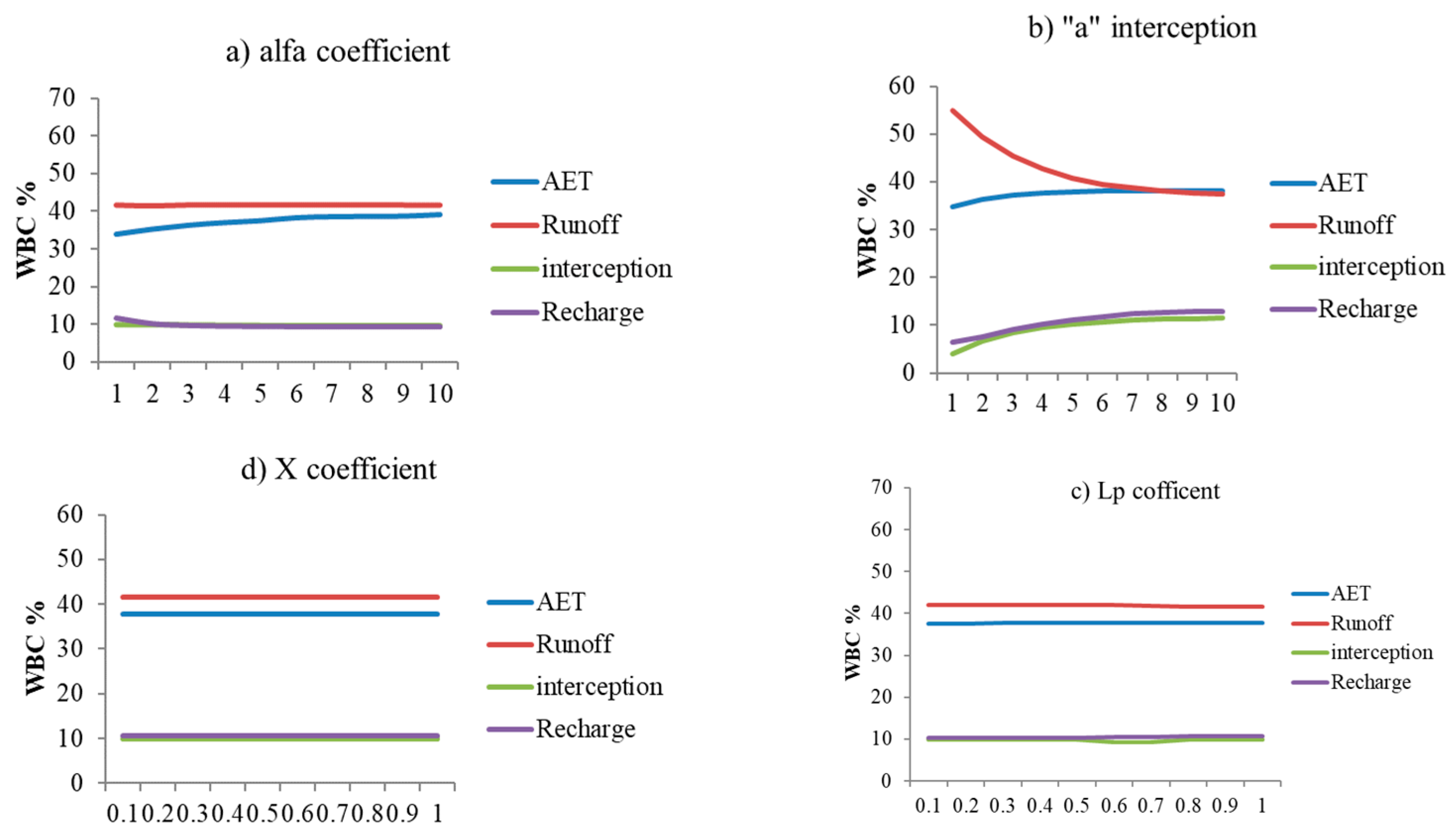
3.4. Model Sensitivity Analysis

Identifying the model parameters that have the greatest influence on the catchment process is vital for understanding the catchment process and evaluating the anticipated uncertainties. The model WetSpass-M classifies its variables into two unique categories: local variables, encompassing aspects such as slope, land use, and soil characteristics, and global variables, encompassing interception, alpha factor, Lp factor, and average intensity factor. Analyzing parameter sensitivity involves aggregating average values of meteorological data from the input dataset of the WetSpass-M model. No modifications have been made to the existing biophysical data. A detailed examination was undertaken in order to identify the sensitivity of many factors, including the “a” intercept, alpha coefficient, and Lp coefficient. As a result, a suitable range of values has been determined for these parameters. Each repetition of the experiment increased the parameter values by 1%. All independent variables and other relevant elements remained constant except for the objective parameters. The target variable was incrementally increased from 25% to 100% in order to assess the impact of changes in the input variable on the different components of the water balance. The remaining variable, however, was maintained at a constant level. Figure 12 illustrates the water balance component’s (WBC) response to variations in the parameters and input variables. Three key input variables were incorporated into the Wabe River watershed model simulation: land-use factors, rainfall intensity, and interceptions. Analyzing the global parameters of the model, it becomes apparent that the components related to the balance between white blood cells (WBC) and water are highly sensitive.

3.5. Model Performance Analysis

3.5.1. Model Calibration

Simulated GWR elements were compared with analytical and graphical assessments of the model’s performance. When selecting the model parameters, the objective was to minimize the discrepancy between observed and simulated values. Model parameters (Table 3) were estimated by manual calibration, which involved generating many samples from the range. The model’s results indicate that the annual runoff volume in the Wabe catchment ranges from 306 mm to 1615 mm, representing the smallest and highest values, respectively. Furthermore, the average depth ratio is calculated to be 468.64 mm. In the catchment area, the mean value represents approximately 34.1% of the annual precipitation. A typical catchment’s runoff value varies by 358.9 mm in summer and 231.4 mm in winter.

3.5.2. Model Sensitivity Analysis

WetSpass-M was used to simulate the volumetric ratio of surface runoff and base flow to streams. Several parameters are included in the model, including the “X” runoff delay factor, the “a” interceptor, the “alpha coefficient,” and the “Lp coefficient.” The parameters were iteratively adjusted at the outlet point of the Wabe River gauge station until a satisfactory agreement was achieved between the simulated and measured flow data. The parameters that were constrained in this study include the runoff delay factor (X) with a value of 0.57, the optimal soil moisture alpha coefficient (X) with a value of 9.5, the Lp value of 0.1, the interception parameter (a) with a value of 9.5, and the correlation coefficient determination (R2) with a value of 0.99. Correlation coefficients may range from 1 to 1. A correlation coefficient (R2) between 0.5 and 0.7 indicates a medium level of connection (Figure 13).
In contrast, an R2 value greater than 0.7 indicates a high correlation. In addition, a coefficient of determination of −1 indicates a negative correlation, whereas a value of 0 indicates no correlation between the two variables. Figure 13 shows that there is a correlation between the measured and simulated flow data. A comparison of the simulated and observed average monthly flow data is illustrated in Figure 14. Therefore, our findings align with the established range of statistically significant positive associations, thus meeting the acceptable threshold. Based on observed stream discharge data, the simulated models’ surface runoff and baseflow parameters were determined.

3.5.3. Model Comparison

Scholars studied the water balance components of different watersheds with similar geological and climatic conditions to those of the present study area in Ethiopia. The simulated values for surface runoff and AET are similar to those found by Wakijra (2020) in the Walga catchment, which were approximately 54.22% and 38.25% of the annual precipitation, respectively. Average annual interception, groundwater recharge, surface runoff, and AET were 36.4 mm, 127.34 mm, 614.95 mm, and 517.59 mm, respectively, in the Bilate Basin, Ethiopia [44]. Similarly, 59.76% of AET, 20.6% of surface runoff, and 19.65% of annual precipitation recharge were calculated by [17]. Only 12% of the precipitation in the Illala catchment recharges the groundwater system; the remaining 81% is lost through Et, and 7% produces surface runoff [20]. Therefore, the WetSpass model produced results equivalent to those of other methods; hence, the result is very comparable to this study result.

4. Conclusions

In this study, groundwater recharge was estimated using the GIS-based WetSpass-M model. WetSpass is a physically distributed hydrological model that assumes a quasi-steady state. Several water balance variables, including GWR, AET, interception, and surface runoff, are estimated during long-term average seasonal and annual periods. Various distributed hydrological models are developed using GIS and RS. Input parameters were interpreted and visualized through the use of GIS. As a result of the WetSpass-M model, groundwater recharge areas were detected, evapotranspiration was quantified, and surface runoff was estimated. Under both annual and seasonal conditions, the WetSpass-M model was successfully used to assess groundwater recharge in the Wabe basin. The model indicates that groundwater recharge and other water balance components vary across time and space due to changes in soil texture, land use and cover, physiography, slope, and hydro-meteorological catchment characteristics.
According to the results, the summer, winter, and average annual groundwater recharge values for the Wabe watershed are 125.5 mm, 78.98 mm, and 204.51 mm, respectively. A precipitation model indicates that summer seasons account for 86.5% of annual precipitation, whereas winter seasons account for 13.5%. Groundwater, on the other hand, facilitates the percolation of approximately 14.8% of the total annual precipitation, a total of 1374.26 mm. ET and surface runoff rates for the Wabe catchment were calculated to be 701.11 mm and 485.58 mm, respectively. There is an observation that 51% of the total precipitation loss is attributed to ET, while 34.1% is attributed to surface runoff.
Sensitivity analyses were conducted on several input components, revealing that most of the factors in the Wabe watershed are sensitive. According to the study, rainfall, PET, and slope significantly influence the quantity and rate of the different components of the water balance. A significant influence is similarly exerted by evapotranspiration to that observed in the parameter sensitivity analysis. There is a noteworthy degree of sensitivity in the coefficients of Lp, alpha, and the intercept. To calibrate the water balance components of the Wabe catchment, both measured and simulated values were used. A good fit was demonstrated between the simulated outputs of the WetSpass-M model and the observed long-term average catchment values. As indicated by an R2 value of 0.99, it is evident that the measured and simulated values exhibit a strong match when the model parameters are changed. Most precipitation is reintegrated into the hydrological cycle via ET, while the remainder contributes to runoff and groundwater replenishment. Northwestern regions of the research area exhibit elevated topography and are characterized by high groundwater recharges, which interact with natural forests. The Wabe catchment area, therefore, effectively supports a dependent groundwater reservoir, with present extraction activities representing only 14.8% of the annual replenishment of groundwater.

Author Contributions

Conceptualization, G.T. and M.J.; methodology, G.T.; software, G.T.; validation, G.T.; formal analysis, G.T.; investigation, M.J.; resources, G.T.; data curation, G.T.; writing—original draft preparation, G.T.; writing—review and editing, M.J.; visualization, G.T.; supervision, M.J. All authors have read and agreed to the published version of the manuscript.

Funding

This research received no external funding.

Data Availability Statement

Data are contained within the article.

Conflicts of Interest

The authors declare no conflicts of interest.

References

  1. Nhemachena, C.; Nhamo, L.; Matchaya, G.; Nhemachena, C.R.; Muchara, B.; Karuaihe, S.T.; Mpandeli, S. Climate change impacts on water and agriculture sectors in southern africa: Threats and opportunities for sustainable development. Water 2020, 12, 2673. [Google Scholar] [CrossRef]
  2. Liersch, S.; Tecklenburg, J.; Rust, H.; Dobler, A.; Fischer, M.; Kruschke, T.; Koch, H.; Hattermann, F.F. Are we using the right fuel to drive hydrological models? A climate impact study in the Upper Blue Nile. Hydrol. Earth Syst. Sci. 2018, 22, 2163–2185. [Google Scholar] [CrossRef]
  3. Gebremeskel, G.; Kebede, A. Estimating the effect of climate change on water resources: Integrated use of climate and hydrological models in the Werii watershed of the Tekeze river basin, Northern Ethiopia. Agric. Nat. Resour. 2018, 52, 195–207. [Google Scholar] [CrossRef]
  4. Tigabu, T.B.; Wagner, P.D.; Hörmann, G.; Kiesel, J.; Fohrer, N. Climate change impacts on the water and groundwater resources of the Lake Tana Basin, Ethiopia. J. Water Clim. Chang. 2021, 12, 1544–1563. [Google Scholar] [CrossRef]
  5. Stathi, E.; Kastridis, A.; Myronidis, D. Analysis of Hydrometeorological Characteristics and Water Demand in Semi-Arid Mediterranean Catchments under Water Deficit Conditions. Climate 2023, 11, 137. [Google Scholar] [CrossRef]
  6. Thornthwaite, C.W. An Approach toward a Rational Classification of Climate. Geogr. Rev. 1948, 38, 55–94. [Google Scholar] [CrossRef]
  7. Nannawo, A.S.; Lohani, T.K.; Eshete, A.A. Envisaging the actual evapotranspiration and elucidating its effects under climate change scenarios on agrarian lands of bilate river basin in Ethiopia. Heliyon 2022, 8, e10368. [Google Scholar] [CrossRef]
  8. Andualem, T.G.; Demeke, G.G.; Ahmed, I.; Dar, M.A.; Yibeltal, M. Groundwater recharge estimation using empirical methods from rainfall and streamflow records. J. Hydrol. Reg. Stud. 2021, 37, 100917. [Google Scholar] [CrossRef]
  9. Davidson, A. The Omo river project, reconnaissance geology and geochemistry of parts of Ilubabor, Kefa, Gemu Gofa and Sidamo, Ethiopia. Ethiop. Inst. Geol. Surv. Bull. 1983, 2, 1–89. [Google Scholar]
  10. Sahle, M.; Saito, O.; Fürst, C.; Demissew, S.; Yeshitela, K. Future land use management effects on ecosystem services under different scenarios in the Wabe River catchment of Gurage Mountain chain landscape, Ethiopia. Sustain. Sci. 2019, 14, 175–190. [Google Scholar] [CrossRef]
  11. Guduru, J.U.; Jilo, N.B. Groundwater potential zone assessment using integrated analytical hierarchy process-geospatial driven in a GIS environment in Gobele watershed, Wabe Shebele river basin, Ethiopia. J. Hydrol. Reg. Stud. 2022, 44, 101218. [Google Scholar] [CrossRef]
  12. Stathi, E.; Kastridis, A.; Myronidis, D. Analysis of Hydrometeorological Trends and Drought Severity in Water-Demanding Mediterranean Islands under Climate Change Conditions. Climate 2023, 11, 106. [Google Scholar] [CrossRef]
  13. Bahir, M.; Ouhamdouch, S.; Ouazar, D.; El Moçayd, N. Climate change effect on groundwater characteristics within semi-arid zones from western Morocco. Groundw. Sustain. Dev. 2020, 11, 100380. [Google Scholar] [CrossRef]
  14. Walker, D.; Parkin, G.; Schmitter, P.; Gowing, J.; Tilahun, S.A.; Haile, A.T.; Yimam, A.Y. Insights from a multi-method recharge estimation comparison study. Groundwater 2018, 57, 245–258. [Google Scholar] [CrossRef] [PubMed]
  15. Sophocleous, M.A. Combining the soilwater balance and water-level fluctuation methods to estimate natural groundwater recharge: Practical aspects. J. Hydrol. 1991, 124, 229–241. [Google Scholar] [CrossRef]
  16. Wang, B.; Jin, M.; Nimmo, J.R.; Yang, L.; Wang, W. Estimating groundwater recharge in Hebei Plain, China under varying land use practices using tritium and bromide tracers. J. Hydrol. 2008, 356, 209–222. [Google Scholar] [CrossRef]
  17. Manghi, F.; Mortazavi, B.; Crother, C.; Hamdi, M.R. Estimating Regional Groundwater Recharge Using a Hydrological Budget Method. Water Resour. Manag. 2009, 23, 2475–2489. [Google Scholar] [CrossRef]
  18. El-Rawy, M.; Zlotnik, V.A.; Al-Raggad, M.; Al-Maktoumi, A.; Kacimov, A.; Abdalla, O. Conjunctive use of groundwater and surface water resources with aquifer recharge by treated wastewater: Evaluation of management scenarios in the Zarqa River Basin, Jordan. Environ. Earth Sci. 2016, 75, 1–21. [Google Scholar] [CrossRef]
  19. Moon, S.-K.; Woo, N.C.; Lee, K.S. Statistical analysis of hydrographs and water-table fluctuation to estimate groundwater recharge. J. Hydrol. 2004, 292, 198–209. [Google Scholar] [CrossRef]
  20. Noor, Q.S.; Thair, S.K. Average monthly recharge, surface runoff, and actual evapotranspiration estimation using WetSpass-M model in Low Folded Zone, Iraq. Open Eng. 2023, 13, 20220451. [Google Scholar] [CrossRef]
  21. Al Kuisi, M.; El-Naqa, A. GIS based spatial groundwater recharge estimation in the Jafr basin, Jordan: Application of WetSpass models for arid regions. Rev. Mex Cienc. Geol. 2013, 30, 96–109. [Google Scholar]
  22. Batelaan, O.; DeSmedt, F. WetSpass: A flexible, GIS-based, distributed recharge methodology for regional groundwater modelling. Impact Hum. Act Groundw Dyn. 2001, 269, 11–17. [Google Scholar]
  23. Anteneh, Z.S.; Awoke, B.G.; Reda, T.M.; Ramasamy, M.J. Spatio-temporal evaluation of water balance components using WetSpass model: In the case of Ataye watershed, Middle Awash Basin, Ethiopia. Arab. J. Geosci. 2023, 16, 1–22. [Google Scholar] [CrossRef]
  24. Danebo, D.; Atilebachew, A.; Abebe, A.; Jothimani, M. Applications of Geospatial Technologies and Wetspass Model in Groundwater Recharge Estimation in Sana River Catchment, Kembata Tembaro Zone, Southern Ethiopia. In Recent Advances in Civil Engineering; CTCS 2021. Lecture Notes in Civil Engineering; Nandagiri, L., Narasimhan, M.C., Marathe, S., Eds.; Springer Nature: Singapore, 2023; p. 256. [Google Scholar]
  25. Wang, L.; ODochartaigh, B.; Macdonald, D. A Literature Review of Recharge Estimation and Groundwater Resource Assessment in Africa; British Geological Survey, 2010; p. 51. Available online: https://nora.nerc.ac.uk/id/eprint/14145 (accessed on 5 December 2023).
  26. Tilahun, K.; Merkel, B.J. Estimation of groundwater recharge using a GIS-based distributed water balance model in Dire Dawa, Ethiopia. Hydrogeol. J. 2009, 17, 1443–1457. [Google Scholar] [CrossRef]
  27. Arefaine, T.; Nedaw, D.; Gebreyohannes, T. Groundwater recharge, evapotranspiration and surface runoff estimation using WetSpass modeling method in Illala Catchment Northern Ethiopia. Momona Ethiop. J. Sci. 2012, 4, 96–110. [Google Scholar]
  28. Armanuos, A.M.; Negm, A.; Yoshimura, C.; Valeriano, O.C.S. Application of WetSpass model to estimate groundwater recharge variability in the Nile Delta aquifer. Arab. J. Geosci. 2016, 9, 1–14. [Google Scholar] [CrossRef]
  29. Dereje, B.; Nedaw, D. Groundwater recharge estimation using WetSpass modeling in Upper Bilate Catchment Northern Ethiopia. Momona Ethiop. J. Sci. 2019, 11, 37–51. [Google Scholar] [CrossRef]
  30. Gebremeskel, G.; Kebede, A. Spatial estimation of long-term seasonal and annual groundwater resources: Application of WetSpass model in the Werii watershed of the Tekeze River Basin, Ethiopia. Phys. Geogr. 2017, 38, 338–359. [Google Scholar] [CrossRef]
  31. Edamo, M.L.; Bushira, K.M.; Ukumo, T.Y.; Ayele, M.A.; Alaro, M.A.; Borko, H.B. Effect of climate change on water availability in Bilate catchment, Southern Ethiopia. Water Cycle 2022, 3, 86–99. [Google Scholar] [CrossRef]
  32. Ukumo, T.Y.; Lohani, T.K.; Edamo, M.L.; Alaro, M.A.; Ayele, M.A.; Borko, H.B. Application of regional climatic models to assess the performance evaluation of changes on flood frequency in Woybo catchment, Ethiopia. Adv. Civ. Eng. 2022, 16, 3351375. [Google Scholar] [CrossRef]
  33. Worku, G.; Teferi, E.; Bantider, A.; Dile, Y.T. Statistical bias correction of regional climate model simulations for climate change projection in the Jemma sub-basin, upper Blue Nile Basin of Ethiopia. Theor. Appl. Clim. 2020, 139, 1569–1588. [Google Scholar] [CrossRef]
  34. Thorntwaite, C.W.; Mather, J. Instructions and Tables for Computing Potential Evapotranspiration and the Water Balance. Laboratory of Climatology. Publ. Climatol. 1957, 10, 311. [Google Scholar]
  35. Wakjira, T. Groundwater Recharge Estimation and Aquifer Characterization for Walga Catchment. Master’s Thesis, Addis Ababa University, Addis Ababa, Ethiopia, 2020. [Google Scholar]
  36. Trajkovic, S.; Gocic, M.; Pongracz, R.; Bartholy, J. Adjustment of Thornthwaite equation for estimating evapotranspiration in Vojvodina. Theor. Appl. Clim. 2019, 138, 1231–1240. [Google Scholar] [CrossRef]
  37. Pereira, A.R.; Pruitt, W.O. Adaptation of the Thornthwaite scheme for estimating daily reference evapotranspiration. Agric. Water Manag. 2004, 66, 251–257. [Google Scholar] [CrossRef]
  38. Yadeta, D.; Kebede, A.; Tessema, N. Potential evapotranspiration models evaluation, modelling, and projection under climate scenarios, Kesem sub-basin, Awash River basin, Ethiopia. Model. Earth Syst. Environ. 2020, 6, 2165–2176. [Google Scholar] [CrossRef]
  39. Shaw, E. Hydrology in Practice; CRC Press: Boca Raton, FL, USA, 2005. [Google Scholar]
  40. Ahmadi, T.; Ziaei, A.N.; Rasoulzadeh, A.; Davary, K.; Esmaili, K.; Izady, A. Mapping groundwater recharge areas using CRD and RIB methods in the semi-arid Neishaboor Plain, Iran. Arab. J. Geosci. 2014, 8, 2921–2935. [Google Scholar] [CrossRef]
  41. Gebreyohannes, T.; De Smedt, F.; Walraevens, K.; Gebresilassie, S.; Hussien, A.; Hagos, M.; Amare, K.; Deckers, J.; Gebrehiwot, K. Application of a spatially distributed water balance model for assessing surface water and groundwater resources in the Geba basin, Tigray, Ethiopia. J. Hydrol. 2013, 499, 110–123. [Google Scholar] [CrossRef]
  42. Abu-Saleem, A. Estimation of Water Balance Components in the Hasa Basin with GIS Based–WetSpass Model. Master’s Thesis, Al Balqa Applied University, Salt, Jordan, 2010. [Google Scholar] [CrossRef]
  43. Ferede, M.; Haile, A.T.; Walker, D.; Gowing, J.; Parkin, G. Multi-method groundwater recharge estimation at Eshito micro-watershed, Rift Valley Basin in Ethiopia. Hydrol. Sci. J. 2020, 65, 1596–1605. [Google Scholar] [CrossRef]
  44. Nannawo, A.S.; Lohani, T.K.; Eshete, A.A. Exemplifying the Effects Using WetSpass Model Depicting the Landscape Modifications on Long-Term Surface and Subsurface Hydrological Water Balance in Bilate Basin, Ethiopia. Adv. Civ. Eng. 2021, 2021, 7283002. [Google Scholar] [CrossRef]
Figure 1. Location map of the study area.
Earth 05 00002 g001
Figure 2. Drainage and topography map of the study area.
Earth 05 00002 g002
Figure 3. Slope map of the study area.
Earth 05 00002 g003
Figure 4. Thiessen polygon map of Wabe catchment.
Earth 05 00002 g004
Figure 5. Average rainfall maps ((a) summer, (b) winter, and (c) annual) of the Wabe catchment.
Earth 05 00002 g005
Figure 6. Average potential evapotranspiration ((a) summer, (b) winter, and (c) annual) of Wabe catchment.
Earth 05 00002 g006
Figure 7. Seasonal and annual average wind speed maps ((a) summer, (b) winter, and (c) annual) of Wabe catchment.
Earth 05 00002 g007
Figure 8. Groundwater level map.
Earth 05 00002 g008
Figure 9. Actual evapotranspiration maps ((a) summer, (b) winter, and (c) annual) of Wabe catchment.
Earth 05 00002 g009
Figure 10. Surface runoff maps ((a) summer, (b) winter, and (c) annual) of Wabe catchment.
Earth 05 00002 g010
Figure 11. Groundwater recharge maps ((a) summer, (b) winter, and (c) annual) of the Wabe catchment.
Earth 05 00002 g011
Figure 12. Sensitivity of global WetSpass-M model parameters on water balance components.
Earth 05 00002 g012
Figure 13. The correlation between measured and simulated flow data.
Earth 05 00002 g013
Figure 14. Comparison between simulated and observed average monthly flow data.
Earth 05 00002 g014
Table 1. Location, elevation, and class type of the meteorological stations within and surrounding the study area.
Location
S.NoStation NameEasting (m)Northing (m)Elevation (m)Station Type
1Welkite37.79118.26911884Class 3
2Gunchire37.84448.244442099Class 3
3Emdibir37.96158.16172082Class 1
4Weliso37.97078.5352028Class 3
5Agena38.1988.19822310Class 3
6Kokir38.238898.4638892613Class 3
7Bui38.3628.2862054Class 1
8Butajira38.31148.1652074Class 3
Table 2. Areal means precipitation depth calculated using the Thiessen polygon method.
Station NameArea (km2)Weighted Area (%)Rainfall (mm)Weighted Rainfall (mm)
Agena44524.21500.4362.9
Kokirgedebano44424.11766.8426.3
Emdibir26714.51225.1177.8
Bui22412.31043.8127.1
Welkite19410.51131.8119.33
Gunchire19210.41370.9143.1
Weliso522.81220.134.5
Butajira221.21075.212.9
Table 3. The standard ranges of WetSpass-M global and local model parameters.
Model ParameterDescriptionUnitsRange Values
LPSoil moisture factor at which AET and PET are at equilibrium-0.1–1
aInterception thresholdmm/day>0.25
αNon-linearity coefficient related to evaporative efficiency->0.9
ΙLong-term average rainfall intensity during wet daysmm/h>0
ω1Slope factor contribution to runoff-0–1
ω2Land use contribution factor to runoff-0–1
ω3Soil factor contribution to runoff-0–1
xRunoff routing delay factor-0–1
βGroundwater recharge storage parameter-0–1
ϕGroundwater recharge contribution parameter to current base-flow-0–1
Disclaimer/Publisher’s Note: The statements, opinions and data contained in all publications are solely those of the individual author(s) and contributor(s) and not of MDPI and/or the editor(s). MDPI and/or the editor(s) disclaim responsibility for any injury to people or property resulting from any ideas, methods, instructions or products referred to in the content.

