Article

Use of Satellite Data for Air Pollution Modeling in Bulgaria

1
Department of Meteorology, National Institute of Meteorology and Hydrology, 1784 Sofia, Bulgaria
2
Space Research and Technology Institute, Bulgarian Academy of Sciences, 1113 Sofia, Bulgaria
*
Author to whom correspondence should be addressed.
Earth 2021, 2(3), 586-604; https://doi.org/10.3390/earth2030034
Submission received: 20 July 2021 / Revised: 27 August 2021 / Accepted: 30 August 2021 / Published: 2 September 2021

Abstract

:
Air pollution continues to be of concern for Bulgarian cities, mainly due to particulate matter of aerodynamic diameter smaller than 10 μm (PM10). There is public and expert interest in the improvement of two operational air quality modeling systems: the Bulgarian Chemical Weather Forecast System (BgCWFS) and the Local Air Quality Management System (LAQMS) for the city of Plovdiv. The aim of the study is to investigate the effects of satellite data assimilation in BgCWFS on surface concentrations over Bulgaria (resolution 9 km), to downscale BgCWFS output to LAQMS (resolution 250 m), and to examine effects on PM10 in Plovdiv. Data from the Global Ozone Monitoring Experiment-2 (GOME-2) (MetOP satellites) for aerosols, nitrogen dioxide (NO2), and sulfur dioxide (SO2) were assimilated in BgCWFS using objective analysis. Simulation experiments with and without satellite data were conducted for a summer and a winter month. The comparison to surface observations in the country showed improvement of results when using satellite data, especially in the summer due to mineral dust events captured by satellites. The decrease in the normalized mean bias (NMB) over the two months was 43% (PM10) and 73% (SO2). The LAQMS estimated background contributions to PM10 in the city as 32%. The absolute NMB by LAQMS decreased by 38%.

Graphical Abstract

1. Introduction

Air quality is a key element for the environment, economy, and public health. In Europe, air pollution is today recognized as the most important environmental health risk, with particulate matter (PM), ozone (O3), and nitrogen dioxide (NO2) concentrations exceeding air quality (AQ) standards in many urban areas [1]. In densely populated urban areas, the multiple emission sources in and around the city cause population exposure to polluted air. In most Bulgarian cities, the primary emission sources are traffic and household heating.
In Europe, about 400,000 premature deaths per year are due to population exposure to PM2.5 (PM with a diameter less than 2.5 μm), while for Bulgaria (with a population of about 7 million), this number was 12,500 in 2018 [1]. This fact ranks Bulgaria in one of the top places among the 41 European countries analyzed in [1]. In 2018, 48% of the urban population in 28 European states were exposed to PM10 concentrations (PM with a diameter less than 10 μm) exceeding the annual value of 20 μgm−3, defined as the air quality guideline by the World Health Organization [2]. The percentage of urban population in Bulgaria exposed to PM10 concentrations above the daily limit value of the European Union (50 µgm−3) was 65.4% in 2018 [3].
Despite emission reductions, air pollutant concentrations still remain high, with exceedance leading to long-term urban population exposure to PM [4]. Air quality in Bulgaria continues to be of great concern, posing new requirements and challenges not only to decision-makers, but also to researchers for providing reliable, timely, and detailed information on air pollution levels both at regional and urban scale.
A variety of methods exist for air quality assessment, forecasting, and understanding air pollution processes in different spatio-temporal scales. Analysis of observational data (e.g., ground-based monitoring networks, remote sensing instruments on board of satellites or on the ground), application of statistical methods, application of modeling systems for transport and chemical transformation of pollutants in the atmosphere, and combinations of these are used worldwide. Combining data from different sources is of increasing interest as this leads to more comprehensive assessment of particulate matter and to estimates of effects of emissions reduction scenarios, for example [5,6].
Satellite-derived data have been used in the last decade to investigate various air pollution aspects such as tracking pollutant plumes in support of air quality forecasting, e.g., [7], describing regional emission sources and their trends [8,9,10], improving lateral boundary conditions in regional AQ models [11], chemical data assimilation in forecasting models [12,13,14,15,16], model validation, e.g., [17,18], creating detailed maps of air pollution at ground level [19], and in epidemiological studies to estimate exposure due to particulate matter concentrations [5,20,21,22].
Satellite data have the advantage of covering wide regions in a short time, capturing the transport of natural aerosols (mineral dust, smoke from wildfires). However, they have some drawbacks [7,23]: polar-orbiting satellites provide data for a given region once a day; clouds can lead to gaps in the spatial coverage; and the derived parameters are representative for the columnar abundance and do not necessarily correspond to surface concentrations. One of the important parameters retrieved by instruments on board of satellites is the Aerosol Optical Depth (AOD), which represents the aerosol load in the column from the Earth’s surface to the top of the atmosphere.
Chemical transport models (CTM) are powerful tools for providing concentrations of different pollutants with high spatial and temporal resolution. Furthermore, they can estimate the effect of emission scenarios on concentrations and are particularly useful for policy support and abatement measures. CTM results, however, exhibit uncertainties related to, among others, the model’s parameterizations and emissions’ input [24]. To improve the accuracy of modeled aerosols, data assimilation of satellite-retrieved AOD has been exploited in the recent years, both for the purposes of forecasting [12,13,25] and analyzing aerosol processes in different geographical areas [26,27].
Data assimilation techniques optimally combine theory (model results) and observations. Methods for chemical data assimilations are discussed in [16,28]. The assimilation of satellite AOD in CTM aims to improve model initial conditions using information not contained in the model emissions (e.g., natural sources of aerosols). The approaches for satellite data assimilation in air quality modeling systems have different levels of complexity (simple optimal interpolation (OI) techniques, Kalman filters, variational methods) [16]. The objective analysis scheme with Cressman successive correction in [29] was beneficial for PM2.5 simulated by a regional CTM over the United States. The application of optimal interpolation led to a decrease in modeled biases by regional scale models over east Asia [23] and the United States [30,31]. State-of-the-art methods are based on variational approaches—3DVAR for assimilation made at a fixed moment [12,13] and 4DVAR for assimilation of a series of observational data [25,32]. Comparable results between 3DVAR and OI are reported in [13].
This study focused on a combination of satellite-retrieved parameters and two air quality modeling systems—a regional one, based on a chemical transport model, and an urban one, with dispersion models for air quality management at city scale.
The Bulgarian Chemical Weather Forecast System, running operationally in Bulgaria since 2012 [33,34,35,36,37], was built upon the WRF-CMAQ model chain (see details in Section 2.2). Evaluation of results upon surface observations indicated underestimations of particulate matter [38]. The local air quality management system (LAQMS) [39,40] was designed and implemented for operational work in the Municipality of Plovdiv (see details in Section 2.5). Plovdiv is the second largest city in Bulgaria (370,000 inhabitants) experiencing high pollution levels and PM exceedances almost during the whole year. Only two regulatory AQ stations are operating in Plovdiv, which does not allow capturing the spatial variability of the air pollution in the city. As there is public and expert concern to enhance the possibilities of the operational modeling systems to better predict PM surface concentrations, both modeling systems were modified to account for satellite-retrieved data in the model’s initial conditions. Satellite data on atmospheric chemistry have not been used in Bulgaria in support of air pollution modeling so far. As a first attempt in this direction, we chose an optimal interpolation technique to improve the chemical initial conditions (IC) in the BgCWFS system.
The main objective of this study was to investigate the effects of satellite data assimilation in BgCWFS on the model’s performance for surface concentrations over Bulgaria (resolution 9 km) during one summer and one winter month. The additional objective was to downscale the BgCWFS output to the finer scale of the LAQMS (resolution 250 m) and to examine the modeled PM10 concentrations in Plovdiv determining the contributions from different emission sources.

2. Materials and Methods

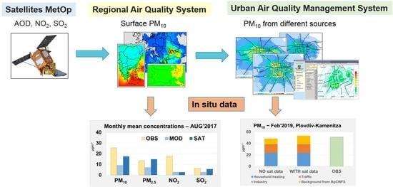
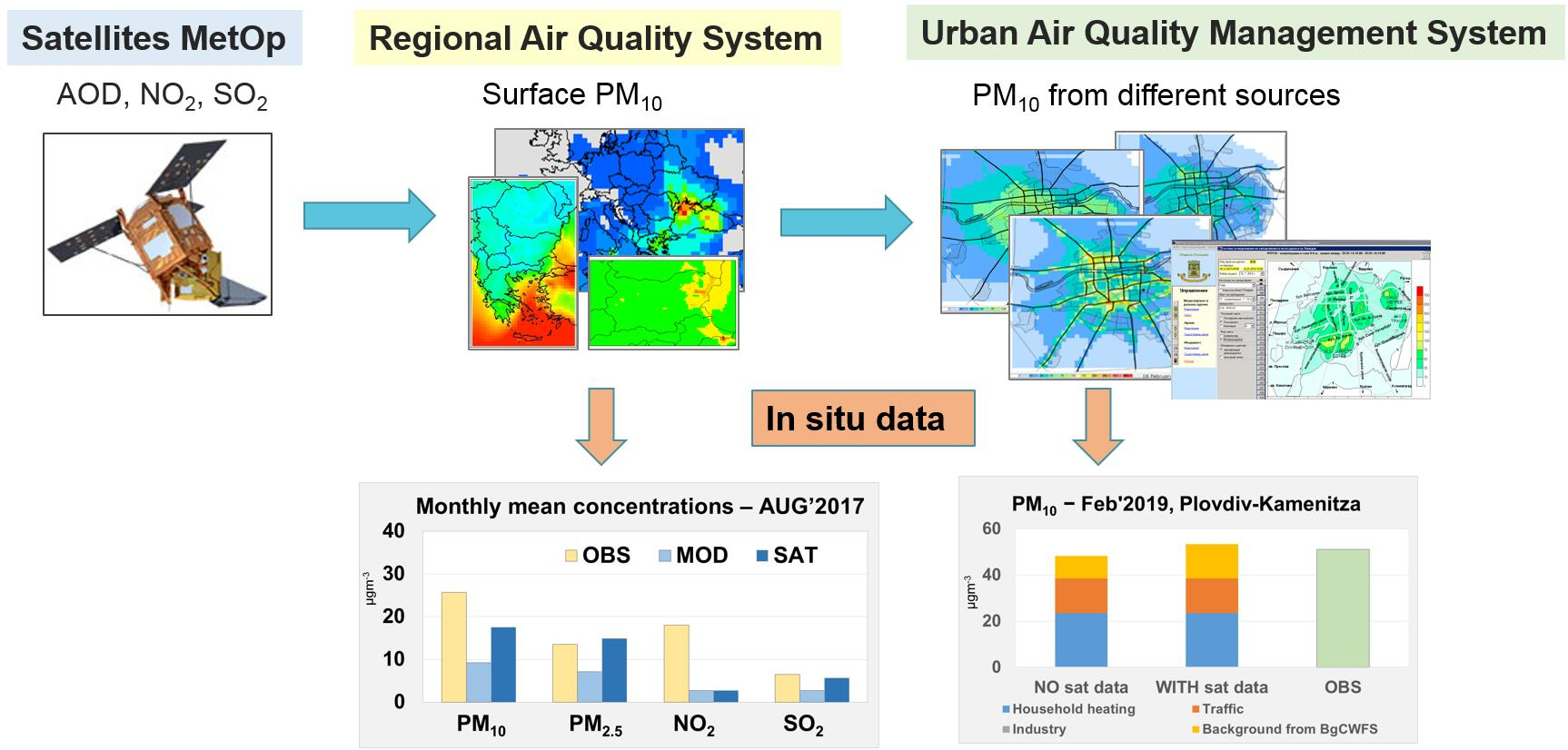
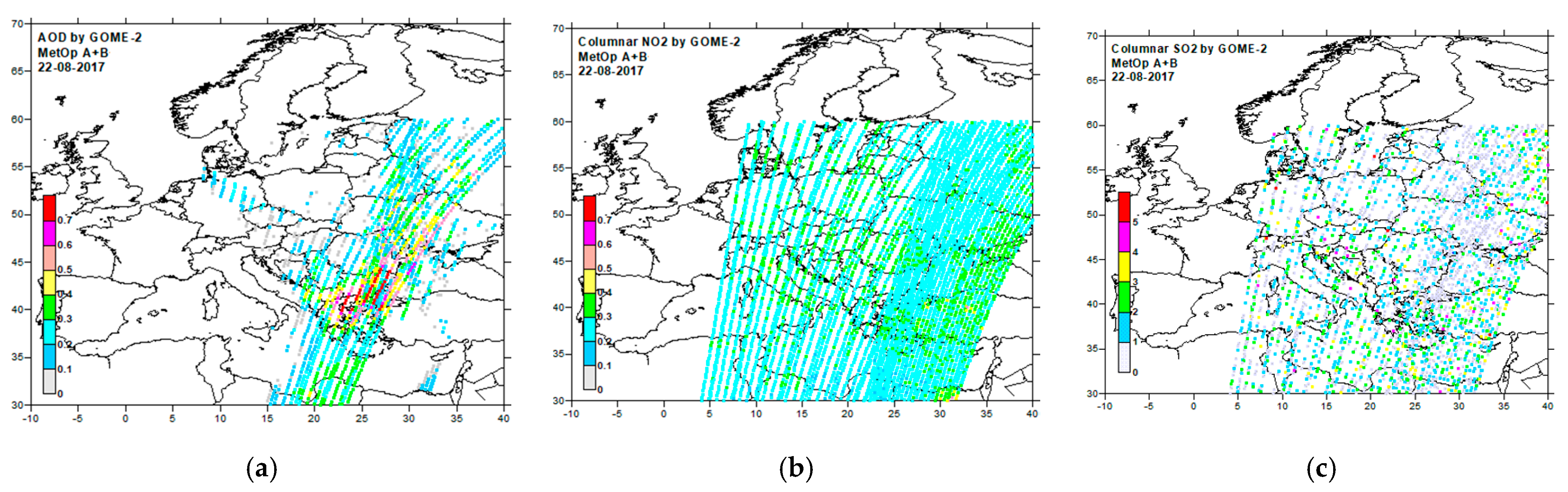
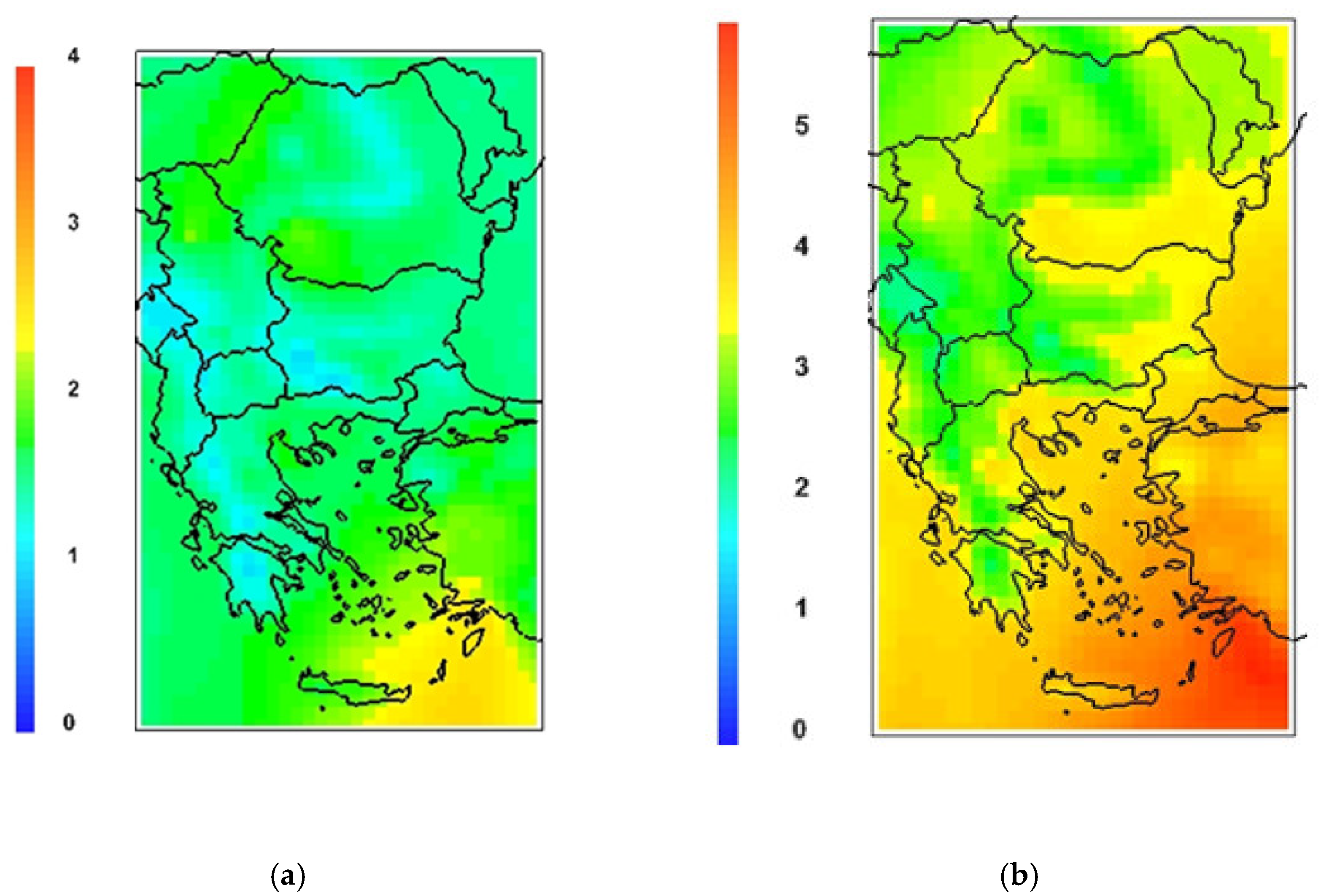
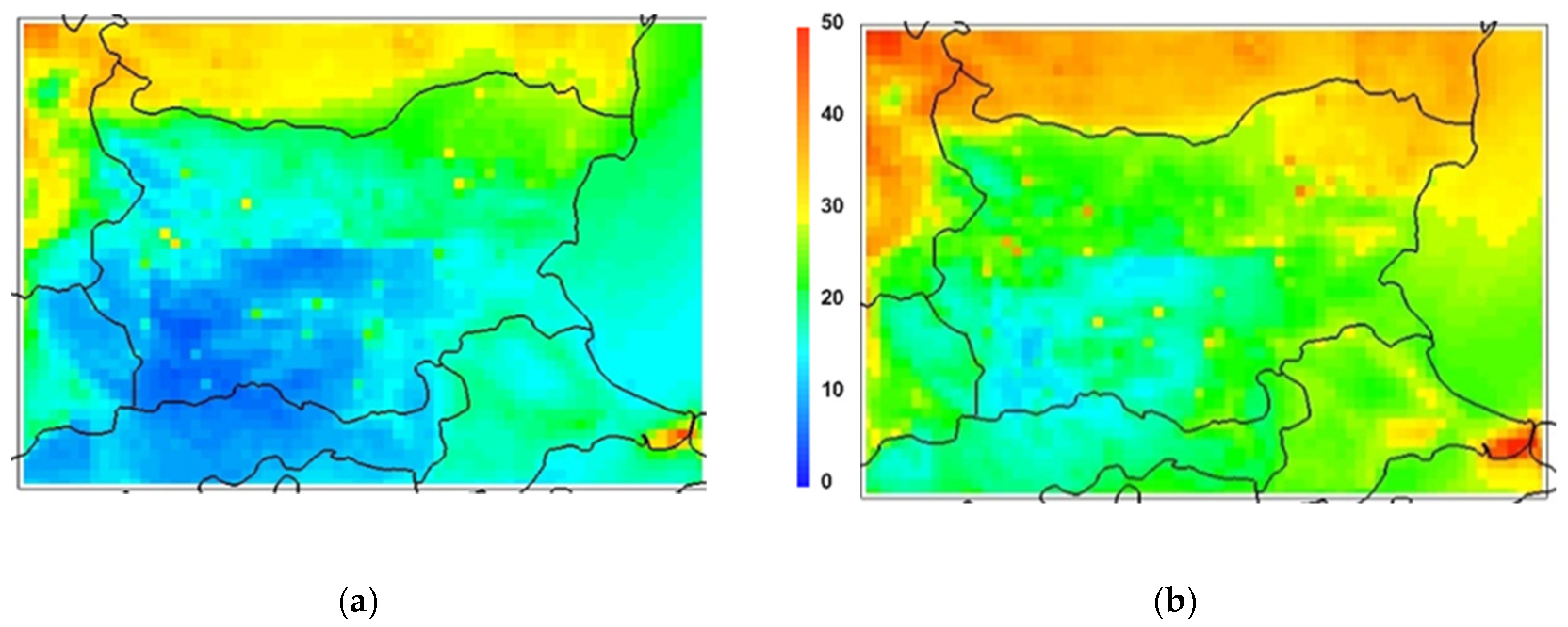
2.1. Satellite Data for AOD, NO2, and SO2

The selection of satellite data to be used in the air pollution system BgCWFS (see Section 2.2) was determined mainly by: (a) the available data for three parameters: aerosol optical properties (aerosol absorbing index AAI, or aerosol optical depth AOD) and the vertical column densities of nitrogen dioxide and sulfur dioxide (VCD_NO2 and VCD_SO2) over the territory of the Balkan Peninsula; and (b) the spatial resolution of the data appropriate for the modeling domains of BgCWFS [41].
Data from the Global Ozone Monitoring Experiment-2 (GOME-2) instrument on board the polar orbiting satellites MetOp A and MetOp B were used in this study, with a possibility to also include MetOp C data. The footprint size is 40 × 40 km2, swath path 960 km (MetOp A, MetOp C) or footprint size 40 × 80 km2, swath path 1920 km (MetOp B). The overpass time for the Balkan Peninsula is around 08–09 UTC, the time difference between MetOp A and MetOp B passage is about 1 h. Level-2 products in .hdf5 format (freely available upon registration at [42]) and in .nc format (freely available at [43]) were post-processed to accommodate BgCWFS model domains and to extract the three parameters to be further used in the modeling system. The data vary by date and parameter; the example in Figure 1 shows the available data on 22.08.2017 in the biggest BgCWFS domain (over Europe).

2.2. The Bulgarian Chemical Weather Forecast System (BgCWFS)

For this study, we used the offline version of the Bulgarian Chemical Weather Forecast System (BgCWFS) [33,34,35,36,37] running operationally at NIMH since 2012. BgCWFS was designed based on the widely used US Environmental Protection Agency (EPA) Models-3 air quality modeling system, including WRF v3.6.1 (Weather Research Forecast model [44], CMAQ v4.6 (Community Multi-scale Air Quality model), an Eulerian chemical transport model [45], MCIP v3.6 (Meteorology-Chemistry Interface Processor), and SMOKE v2.4 (Sparse Matrix Operator Kernel Emissions Modeling System–the emission pre-processor to CMAQ) [46].
BgCWFS is running in five nested domains: the European region (81 km horizontal resolution), the Balkan Peninsula (27 km), Bulgaria (9 km), and two smaller domains around Sofia: Sofia Province (3 km) and Sofia City (1 km).
The emission data in BgCWFS are based on the emission inventory for Europe prepared by the Netherlands Organization for Applied Scientific Research (TNO) for the year 2010 [47] and on the Bulgarian emission inventory for 2015. A Geographic Information System (GIS)-based web-platform was created to grid European and Bulgarian inventory data over the 5 BgCWFS domains. The gridded data are processed by specially designed pre-processor modules which perform temporal allocation and speciation splitting for the area (AS) and large point (LPS) sources. SMOKE is used to estimate the biogenic emissions and to merge them with the AS and LPS ones.
The initial conditions (ICs) and boundary conditions (BCs) for the meteorological calculations are taken from the Global Forecast System (GFS) (weather forecast model) at the National Centers for Environmental Prediction (NCEP) [48] with grid resolution 1° × 1° and temporal resolution of 6 h. The chemical BCs over the outer domain (Europe) are set according to the climatic profiles embedded in the CMAQ software. The presumption is that the possible errors decrease when moving away from the boundaries inside the domain because of dispersion and removal processes, and because of the continuous action of the pollution sources inside the domain. The BCs for each of the other domains are determined from the senior ones.
The vertical structure of CMAQ is determined by fourteen layers of varying thickness between the surface and 100 hPa, with the first layer being between 55 and 60 m thick. The Planetary Boundary Layer (PBL) is presented by the lowest eight levels. The system is set up with well-known and widely accepted parameterization schemes for meteorological processes and chemical mechanisms (see details in [49]). The output of CMAQ contains 3D hourly files for concentrations, depositions, and visibility parameters related to 78 pollutants. Post-processing is carried out to extract the surface concentrations of the main pollutants (e.g., ozone, particulate matter, nitrogen dioxide, etc.) and visualize them as maps on the website of NIMH [50].

2.3. AOD Calculation in BgCWFS

AOD is not a default parameter in CMAQ. For its estimation, five different approaches were analyzed and tested [51]. Four of the methods were embedded in CMAQ. Two of them are based on the estimation of the visibility parameters and the extinction coefficients (Mie theory and reconstruction method), while the other two are based on light extinction for different species, and empirical relationships between visibility parameters and aerosol mass concentrations (algorithm based on data from the Interagency Monitoring of Protected Visual Environments (IMPROVE) monitoring network in the United States). The fifth method is the post-processing tool FlexAOD [52,53], which uses mass concentrations of the speciated aerosol (i.e., sulfate, nitrate, ammonium, black carbon, organic carbon, sea salt, soil dust) and the distribution of the relative humidity. Based on the comparative analysis in [51], the FlexAOD software was selected to estimate AOD at 550 nm (denoted further as AOD) from CMAQ output.

2.4. Assimilation of Satellite-Retrieved Data in BgCWFS

As this was the first attempt to use satellite-retrieved data in BgCWFS, we chose to implement a simple assimilation technique based on optimal interpolation [16,24] and correction of the initial model profiles. The correction factor was calculated as the ratio between BgCWFS vertical column parameters (e.g., AODm estimated by BgCWFS) and the parameters obtained from satellite data (e.g., AODs), and it was further used to modify the profile concentrations, Figure 2. In the case of AOD assimilation, this involved correction of different PM species (type and size mode). The same correction approach was also applied for the vertical column densities of NO2 and SO2.
The assimilation took place in the first three model domains (Europe, the Balkan Peninsula, and Bulgaria) at the time of the satellite overpass hour Hs (fixed at 09:00 UTC). WRF, the meteorological model, was run once at the beginning of the assimilation. CMAQ was run twice: a normal 24-h run and a run with part-day integration from Hs to the end of the day. The assimilation created new concentrations fields used as initial conditions for the next-day runs.

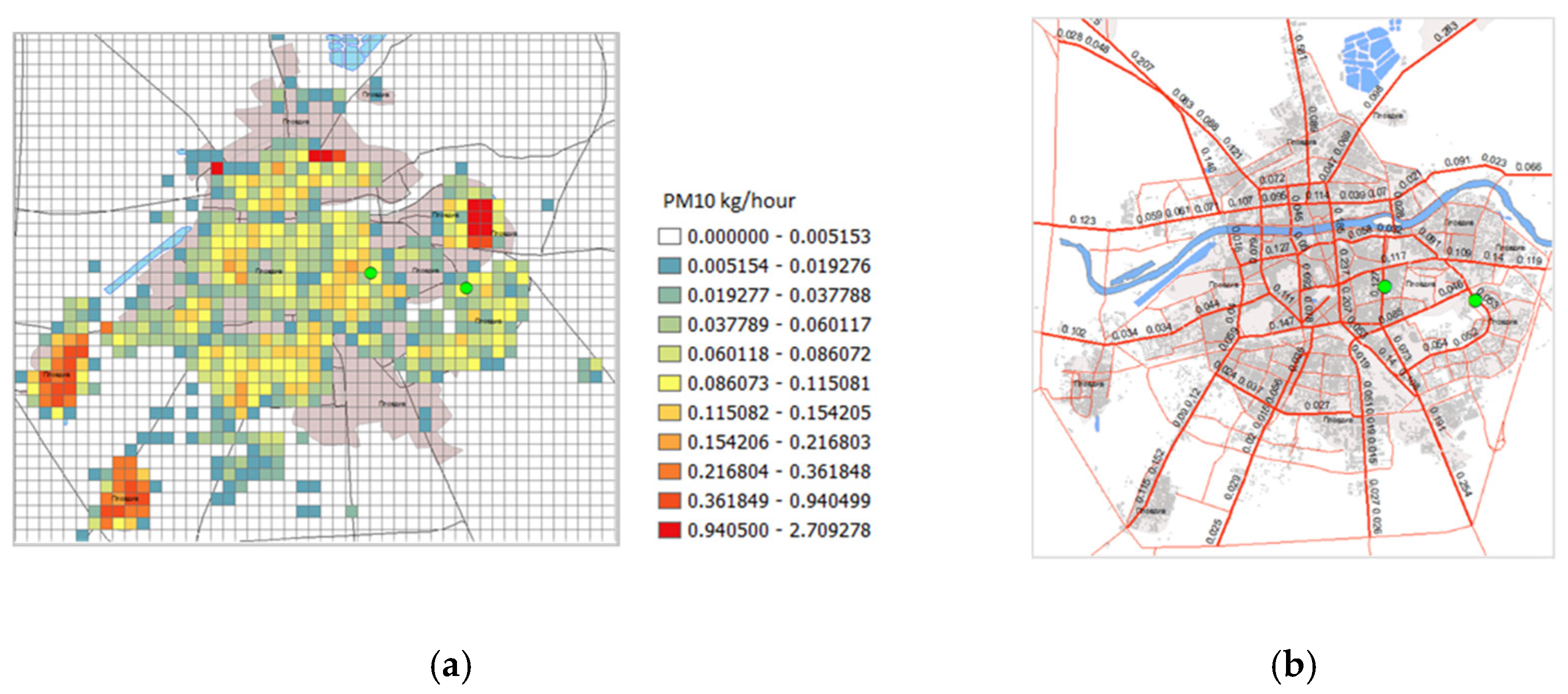
2.5. Local Air Quality Management System (LAQMS)

The LAQMS was developed at NIMH in 2004 as an operational system intended for the authorities of the city of Plovdiv—the second largest city in Bulgaria, experiencing permanent air quality problems in the past decade mainly due to high concentrations of particulate matter. The design of the system was determined by its main objective—to be in support of local authorities to make both short-term and long-term decisions on air quality management. The system was set up for two domains, Plovdiv region (63 km × 44 km with grid resolution of 1 km) and Plovdiv city (12 km × 11 km with grid resolution of 250 m). The LAQMS has four main modules [40]:
  • Meteorological pre-processor modules,
  • Emission modules,
  • Dispersion modules, and
  • Post-processing modules and interface for AQ experts (expert module).
The meteorological pre-processor module was modified so as to receive the output of the WRF model of BgCWFS in domain Bulgaria (resolution 9 km). The emission modules accounted the following pollution sources in the city: household heating, traffic, and industry. For this study, a bottom-up approach [54,55] was applied for the emission inventory of household heating and traffic in Plovdiv. The emissions from household heating were estimated using high-resolution data for the distribution of the households in the city. Details for the type of fuel used and the electricity consumption were obtained based on data from 450 questionnaires distributed among the citizens of Plovdiv. For the emissions from the road transport in the city, data from traffic cameras were analyzed, also applying high resolution mapping of the street network. GIS functionalities were used to automatically perform spatial operations. In Figure 3, the estimated emissions of particulate matter from these two sources are shown.
The dispersion module incorporates two models: Poltran (a combination of an Eulerian advection scheme and numerical calculation of the turbulent diffusion) [39], used as a main dispersion model, and AUSTAL2000 (a Lagrangian type, the reference dispersion model of the German Environment Agency [56]), used as a complement to Poltran regarding dispersion from point and linear sources during the first hour of the simulations.
The LAQMS separately simulates the dispersion of pollutants released from the different groups of emission sources. Thus, the concentrations include concentrations caused by household heating, traffic, and industry in the city, and background concentrations caused by emission sources located outside the city. The effect of satellite data was introduced in LAQMS through the background concentrations. The parameters calculated by BgCWFS_sat for use in the LAQMS included meteorological variables (wind, temperature, etc.) and the concentrations of eight pollutants (NO2, NO, CO, SO2, O3, NH3, PM10, and PM2.5). These parameters were used to determine the background concentrations for the domains of LAQMS.
The expert module of LAQMS is a post-processing tool intended to visualize the spatial distribution of concentrations, due to different groups of emission sources, and to aggregate the hourly values in different time scales (e.g., daily, annual, etc.). Examples can be found in [57].

2.6. Simulations and Evaluation of the Models’ Performance

Simulations with BgCWFS and LAQMS were carried out for two months—August 2017 and February 2019. The periods were chosen so as to represent the summer period and the winter period, also accounting for available GOME-2 data for the Balkan Peninsula (BgCWFS domain 2).
August in Bulgaria is one of the hottest and driest months. August 2017 was characterized by temperatures exceeding the climatic norm by +0.5 °C to +3.9 °C and gross monthly precipitation around the norm. The dry weather was favorable for wildfires, mainly in the south-western and south-eastern regions of the country. The AOD over the country was affected by such fires, but also by Saharan dust outbreaks [43,58]. According to satellite data, higher AOD values were observed on about 12 days in this month. February is usually one of the coldest months in Bulgaria with long-lasting anticyclonic conditions leading to elevated air pollution. February 2019, however, featured mild temperatures (deviation from the monthly climatic norm by 2.1 °C) and less precipitation (deviation from the monthly norm by 52%). The average number of days with clear sky was 10 (higher than the climatic norm); therefore, more satellite data than for other winter months were available.
Simulations were carried out by BgCWFS in offline mode in two versions: “mod” (without assimilation of satellite data) and “sat” (with assimilation of satellite data). The local system, LAQMS, was run for the city of Plovdiv using background concentrations as calculated by BgCWFS_mod and BgCWFS_sat.
To evaluate the model’s results for domain Bulgaria, surface observations for particulate matter (PM10 and PM2.5), SO2, and NO2 at regulatory air quality monitoring stations in Bulgaria were used. The data are freely available in [59]. Only background stations with data availability of more than 75% during the two months were included in the analysis, Figure 4. Some widely used statistical metrics (Appendix A) were calculated for the monthly mean values at all stations, while boxplots and kernel density functions were used to visualize the model’s performance at selected stations: two urban stations in Sofia and Plovdiv, and one rural/mountain station, Sofia-Kopitoto (1321 m.a.s.l.).

3. Results

We discuss results obtained by two versions of BgCWFS: BgCWFS_mod and BgCWFS_sat focusing on the ground-level concentrations for selected pollutants (PM10, PM2.5, NO2, and SO2) and the columnar parameters (AOD and VCD_NO2 and VCD_SO2). The simulations were carried out for two months. Surface observations from the AQ monitoring network in Bulgaria were used to check BgCWFS performance. At urban scale, for the city of Plovdiv, LAQMS results for PM10 are shown, analyzing the contribution of BgCWFS background values to the monthly mean concentrations at the two AQ stations in Plovdiv.

3.1. BgCWFS_mod vs. BgCWFS_sat

The hourly time evolution of the differences (sat − mod) displayed typical spatial distribution pattern for all pollutants. At the time of satellite overpass hour (fixed at Hs = 09:00 UTC), disturbances that resembled area pollution source were noticed in the fields. These disturbances evolved with time due to atmospheric transport and transformations, changing position and decreasing in magnitude [49]. As examples of the spatial distribution of monthly mean values, in Figure 5 AOD in BgCWFS domain Balkan Peninsula for August 2017 and in Figure 6 PM10 in model domain Bulgaria for February 2019 are shown. The AOD map by BgCWFS_sat indicated higher values, especially in the southern and eastern parts, associated with the frequent Saharan dust outbreaks in August which approached Bulgaria from the south-west and moved towards the north-east. The corresponding maps for PM10 and PM2.5 in domain Bulgaria (Figure S1) featured increased values from BgCWFS_sat in the eastern part of the country and the adjacent Black Sea area. The NO2 and SO2 maps (Figure S2) displayed higher values for big urbanized and industrial areas. The assimilation of satellite data led to noticeable overall increase of SO2 in the domain with apparently no effect on NO2 concentrations.
The map for PM10 over Bulgaria in February 2019 from BgCWFS_sat (Figure 6b) indicated an overall increase in surface PM10 concentrations compared to the map from BgCWFS_mod, especially in the northern part of the domain. The PM2.5 distribution (Figure S3) was similar to the PM10 distribution, with a noticeable increase in the eastern part of the domain. The NO2 and SO2 maps for this winter month (Figure S4) had the same main features as the maps for the summer month, with a significant increase of SO2 from BgCWFS_sat over the entire domain.
The differences (sat − mod) in the monthly mean values of the surface and columnar parameters averaged over domain Bulgaria are shown in Figure 7. The domain mean concentrations of all parameters from BgCWFS_sat increased (positive differences), except for NO2 (surface and columnar values). The increase for the domain mean PM10 was 7–10 µgm−3, which corresponds to percentage increase from BgCWFS_sat of 117% in August and 42% in February. The pronounced increase in the summer was associated with the frequent Saharan dust intrusions, captured by GOME-2 with good coverage over Bulgaria under low cloudiness conditions. A significant increase of SO2 and VCD_SO2 was also observed, more noticeably for February (161% and 335%, respectively). This is more likely due to higher SO2 emissions in south-eastern Europe in winter resulting from energy production by coal-fired thermal power plants, as indicated by the long-term satellite-derived SO2 data [60]. The impact on NO2 was weak. NO2 is a highly reactive gas originating mainly from transport and combustion sources near the surface. It has a short lifetime (a few hours to one day [61]), it is involved in nonlinear chemistry, and its distribution is characterized by strong horizontal inhomogeneity and well-expressed gradients in the Planetary Boundary Layer (PBL). These peculiarities pose challenges for the assimilation of satellite-retrieved tropospheric NO2 [16]. The weak impact of the assimilation observed in our NO2 model results might be attributed to different reasons: coarse satellite footprint not allowing to reproduce local scale NO2 distribution [62], inappropriate assimilation technique [63], or temporary scale (monthly) analysis that could mask the effects on a daily basis. Results with 4DVAR assimilation in the Integrated Forecasting System (IFS) of the European Center for Medium Range Weather Forecasts (ECMWF) [64] indicate that the small effect of the assimilation of satellite-retrieved tropospheric NO2 columns is due to the short lifetime of NO2.

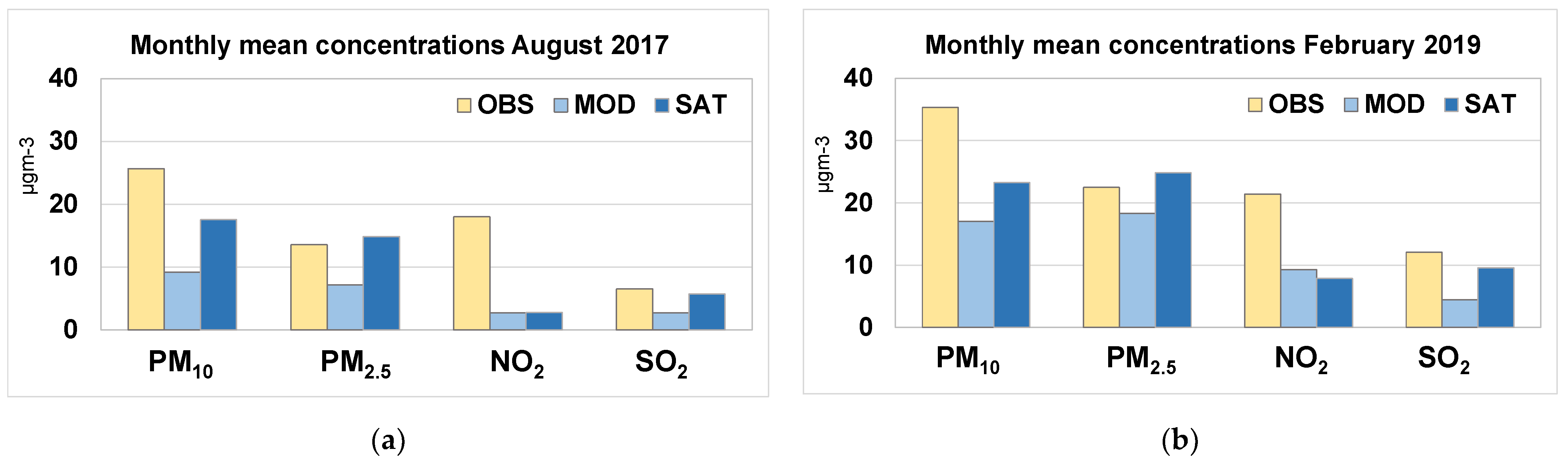
3.2. Comparison of BgCWFS Results to Surface Observations

The results from the two versions of BgCWFS in domain Bulgaria were compared to data from the surface AQ monitoring network for PM10, PM2.5, NO2, and SO2. Table 1 and Table 2 provide statistical parameters (defined in Appendix A) for the monthly mean values based on all available data, respectively for August 2017 and February 2019, while Figure 8 shows the comparison for the monthly mean values. The assimilation of satellite data led to a decrease in the FGE and NMB scores for all pollutants, except NO2 and PM2.5 in February. For PM10, the NMB decreased in BgCWFS_sat more noticeably in August, by ~50%, than in February, by 34%. For SO2, the sat-version showed a decrease in the NMB by 72% on average for the two months. PM2.5 concentrations from BgCWFS_sat were overestimated, more evidently in February, 34%. It should be noted that only 4 stations provided PM2.5 data for this month. NO2 from BgCWFS_mod was strongly underestimated (by a factor of 3 in August). The possible reason might be associated with the ozone overestimation in the summer period found in previous evaluation of BgCWFS_mod [35]. The NO2 underestimation also indicated a deficit in modeled emissions from the traffic. As highlighted for the domain mean NO2 concentrations, the assimilation of satellite data did not lead to improvement at the stations either.
In Figure 9 and Figure 10, the comparison for PM10 and SO2 at three selected stations (see Figure 4) for August 2017 is shown. PM10 values from BgCWFS_sat were underestimated at all stations, but to a lesser extent than the values from BgCWFS_mod (average NMB values −31.7% and −64.3%, respectively). The station with the highest underestimation from BgCWFS_sat (NMB −47% for PM10 and −37% for SO2) was Plovdiv-Kamenitza, which indicates that air pollution at this site was more influenced by local factors, not captured by the system with 9 km resolution. Similar plots for PM2.5 (Figure S5) confirm general improvement from BgCWFS_sat, especially at the urban sites. As already shown by the distribution maps, NO2 was underestimated by both model versions by a factor of 6 on average for the selected stations (Figure S6). For February 2019, the comparison of PM10 and PM2.5 (Figures S7 and S8) showed better matching from BgCWFS_sat compared to the observations at the Sofia-Hipodruma station with absolute value of the NMB less than 8%. For Plovdiv-Kamenitza station, significant underestimation of PM from BgCWFS_sat was still observed (NMB −55% on average). At Sofia-Kopitoto mountain station, PM concentrations from BgCWFS_sat were overestimated by a factor of about 3. At Sofia-Drujba and Plovdiv-Kamenitza stations, NO2 (Figure S9) was underestimated by both model versions with NMB of about −75%. BgCWFS_sat led to clear improvement of SO2 at Plovdiv-Kamenitza station (Figure S10) with NMB decreasing from −64% to −36%. For the other two stations (Sofia-Drujba and Sofia-Kopitoto), the assimilation of satellite data resulted in overestimated SO2 with an average NMB of 55%.

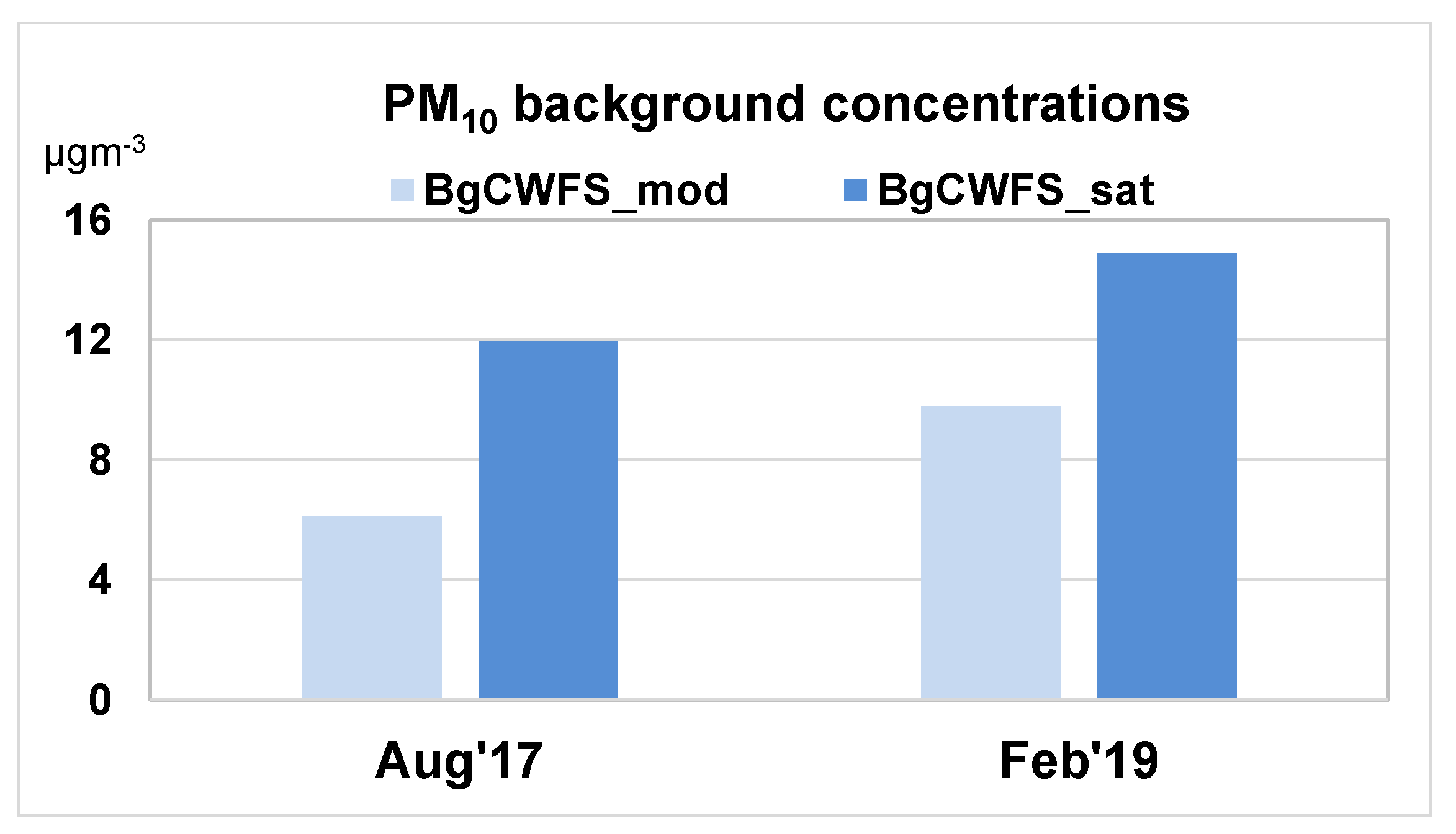
3.3. BgCWFS-LAQMS Results for Plovdiv

The LAQMS simulates surface concentrations of pollutants for the city of Plovdiv due to different emission sources in the city (household heating, traffic, industry) and outside of the city (background concentrations). The background concentrations were provided by BgCWFS_mod and BgCWFS_sat. In the LAQMS domain (size about 10 × 10 km2), the background values from BgCWFS showed negligible changes. Thus, for simulations with LAQMS, the background concentrations, and accordingly the satellite corrections were assumed to be constant within the LAQMS model domain.
The PM10 background concentrations from BgCWFS_sat were significantly higher than those from BgCWFS_mod, as shown by the monthly mean values in Figure 11. The increase in both months was more than 50%.
In Figure 12 and Figure 13, the monthly mean PM10 concentrations for August 2017 and February 2019 are shown. In the winter month, almost the whole domain featured PM10 above 50 µgm−3, with some central parts registering even higher than 100 µgm−3.
In Figure 13, additional information about the main sources contributing to the PM10 concentration in February 2019 is provided. The maps indicate zones with higher concentrations due to household heating and zones where traffic is the major contributor to PM10.
Table 3 and Table 4 show the comparison of modeled to observed PM10 monthly mean values, respectively for August 2017 and February 2019, at the two AQ stations in Plovdiv-Kamenitza (urban background) and Trakia (traffic) (locations marked in Figure 12 and Figure 13). The contribution of BgCWFS_mod background concentrations to the calculated PM10 concentrations for February 2019 was 20% at Kamenitza station and 18.5% at Trakia station. With the use of satellite data, the contribution of BgCWFS_sat background concentration increased to 28% at Kamenitza and to 26% at Trakia. For August 2017, the corresponding numbers using BgCWFS_mod were 24.4% and 21.9%, while for BgCWFS_sat they were, respectively, 38.7% and 35%.
The use of BgCWFS_sat and LAQMS models led to a small overestimation for PM10 at Kamenitza station for the two months (by 8% on average) while at the Trakia traffic station, PM10 remained underestimated, but with a decrease in the NMB (from −23% to −12%).

4. Discussion

Satellite-retrieved data for atmospheric chemistry parameters were used for the first time in Bulgaria in air pollution modeling systems—a regional one, based on a chemical transport model (BgCWFS), and an urban one, designed for local air quality management in the city of Plovdiv (LAQMS). To investigate the effect of satellites data assimilation on surface concentrations in the country and in the city of Plovdiv, BgCWFS was set up in offline mode and modified for the calculation of vertical columnar parameters in the chemical transport model of BgCWFS, for the assimilation of GOME-2 derived data for AOD, VCD_NO2, and VCD_SO2 in the three coarser BgCWFS domains (Europe, the Balkan Peninsula, and Bulgaria). A rather simple approach (objective analysis and correction of pollutants profiles) was used for the satellite data assimilation in BgCWFS at satellite overpass time fixed at 09:00 UTC. The output of BgCWFS at country level (horizontal resolution 9 km) was used to estimate the background concentrations for the LAQMS. Furthermore, the emissions in the city of Plovdiv were updated and clarified using a GIS-based bottom-up emission inventory.
The simulation experiments conducted using the two versions of the system (with and without satellite data), BgCWFS_sat and BgCWFS_mod, for two months (August 2017 and February 2019) showed an increase in the domain mean surface concentrations of PM10, PM2.5, and SO2, while the NO2 values remained almost unchanged. The increase in domain mean PM10 was highest in the summer month (10 µgm−3), where the map for the spatial distribution showed enhanced values especially in the southern and eastern part of the country, corresponding to the mineral dust events with air masses approaching from the south-west and moving towards the north-east. Thus, the assimilation of satellite data provided the possibility to account for emissions not included in BgCWFS. The increase of domain mean SO2 was highest in the winter month (~6 µgm−3) and this is likely due to the relatively high emissions by coal-fired thermal power plants in the Balkan Peninsula. The weak impact of satellites data assimilation on surface and columnar NO2 values confirmed the results in [60].
The comparison of BgCWFS monthly mean surface concentrations to observations at air quality monitoring sites in Bulgaria suggested improvement when using satellite data. The NMB from BgCWFS_sat, averaged over the two months, was lower than the NMB from BgCWFS_mod by 43% (PM10) and 73% (SO2). The monthly mean PM10 values simulated by BgCWFS_sat were still underestimating the observed concentrations in most of the air quality stations. This was expected, as model values are representative for a grid of 9 km, while observations represent local conditions. Interestingly, we noticed a tendency for PM2.5 overestimation which is more likely due to the assimilation approach of correcting profiles of different species. Further analysis is needed to understand this behavior. NO2 concentrations were strongly underestimated by both BgCWFS versions, suggesting a deficit in model emissions.
The LAQMS benefits from the satellite data assimilation through the background concentrations for the Plovdiv domain provided by BgCWFS_sat. The simulation experiments with LAQMS for the two months estimated the PM10 concentrations caused by different emission sources in the city (household heating, traffic, industry) and outside the city through the background concentrations. The LAQMS estimated the contribution of the background concentrations to PM10 at the locations of the two air quality stations in Plovdiv as 32%, averaged for the two months. The absolute value of the NMB decreased from 15.5% (without satellite data) to 9.6% (with satellite data).
The assimilation algorithms developed for GOME-2 retrieved data can be adapted to data from other instruments that have finer spatial resolution (e.g., from the Tropospheric Monitoring Instrument (TROPOMI) on board the Copernicus Sentinel-5 Precursor satellite, TROPOMI-S5p) and could be used for data assimilation in the smaller domains of BgCWFS (e.g., the Sofia region).
Finally, this study is a significant step towards the development of an operational system for assimilation of satellite data over Bulgaria. The presented prototype of the modeling chain BgCWFS-LAQMS is in pre-operative mode. This prototype can be further modified for operational runs, with activities on streaming the satellite dataflow at the overpass time to BgCWFS runs in nested domains and setting up links to LAQMS in near-real time.

Supplementary Materials

The following are available online at https://www.mdpi.com/article/10.3390/earth2030034/s1, Figure S1: Monthly mean values of PM10 and PM2.5 (µgm−3) August 2017: (a) and (c) BgCWFS_mod; (b) and (d) BgCWFS_sat; Figure S2: Monthly mean values of NO2 and SO2 (µgm−3), August 2017: (a) and (c) BgCWFS_mod; (b) and (d) BgCWFS_sat; Figure S3: Monthly mean values of PM2.5 (µgm−3), February 2019: (a) BgCWFS_mod; (b) BgCWFS_sat; Figure S4: Monthly mean values of NO2 and SO2 (gm−3), February 2019: (a) and (c) BgCWFS_mod; (b) and (d) BgCWFS_sat; Figure S5: PM2.5 in August 2017—observed, BgCWFS_sat and BgCWFS_mod at 3 selected stations: (a) Plovdiv-Kamenitza (BG0051A); (b) Sofia-Hipodruma (BG0050A); and (c) Sofia-Kopitoto (BG0070A); top panels—boxplots show minimum, maximum, 25th, 50th, and 75th percentiles, bottom panels—kernel density estimations of the density distribution functions; Figure S6: NO2 in August 2017—observed, BgCWFS_sat and BgCWFS_mod at 3 selected stations: (a) Plovdiv-Kamenitza (BG0051A); (b) Sofia-Drujba (BG0052A); and (c) Sofia-Kopitoto (BG0070A); Figure S7: PM10 in February 2019—observed, BgCWFS_sat and BgCWFS_mod at 3 selected stations: (a) Plovdiv-Kamenitza (BG0051A); (b) Sofia Drujba (BG0052A); and (c) Sofia-Kopitoto (BG0070A); Figure S8: PM25 in February 2019—observed, BgCWFS_sat and BgCWFS_mod at 3 selected stations: (a) Plovdiv-Kamenitza (BG0051A); (b) Sofia-Hipodruma (BG0050A); and (c) Sofia-Kopitoto (BG0070A); Figure S9: NO2 in February 2019—observed, BgCWFS_sat and BgCWFS_mod at 3 selected stations: (a) Plovdiv-Kamenitza (BG0051A); (b) Sofia-Drujba (BG0052A); and (c) Sofia-Kopitoto (BG0070A); Figure S10: SO2 in February 2019—observed, BgCWFS_sat and BgCWFS_mod at 3 selected stations: (a) Plovdiv-Kamenitza (BG0051A); (b) Sofia-Drujba (BG0052A); and (c) Sofia-Kopitoto (BG0070A).

Author Contributions

Conceptualization, E.G., D.A. and T.S.; methodology, D.S., D.A., M.D. and E.G.; software, D.S., D.A. and M.P.; validation, E.G., D.S., D.A., N.N., H.K. and E.H.; formal analysis, E.G., D.S., D.A., H.K. and B.V.; investigation, all authors; data curation, M.D., N.N. and R.N.; writing—original draft preparation, E.G., T.S. and H.K.; writing—review and editing, B.V. and E.H.; visualization, H.K., N.N., D.S., D.A. and A.P. All authors have read and agreed to the published version of the manuscript.

Funding

This research is one of the outcomes of a project funded by the European Space Agency (ESA) under the PECS (Plan for Еurореаn Cooperating States), grant number 4000124150/18/NL/SC.

Data Availability Statement

All relevant data are reported in the paper.

Acknowledgments

Deep gratitude is due to ESA services providing data from the GOME-2 instrument on board the MetOp-A, B and C satellites. The authors are grateful also to the US EPA for providing WRF-CMAQ models, to the TNO for the emission inventory at European scale used in BgCWFS, and to the European Environment Agency for observational data from the surface air quality monitoring network. We acknowledge the use of data and/or imagery from NASA’s Fire Information for Re-source Management System (FIRMS) (https://earthdata.nasa.gov/firms (accessed on 31 August 2021)), part of NASA’s Earth Observing System Data and Information System (EOSDIS).

Conflicts of Interest

The authors declare no conflict of interest. The funders had no role in the design of the study; in the collection, analyses, or interpretation of data; in the writing of the manuscript, or in the decision to publish the results. The views expressed herein саn in nо way be taken to reflect the official opinion of the Еurореаn Space Agency.

Appendix A

Statistical indexes used for comparison of modeled (m) to observed (o) surface concentrations, are estimated as:
StatisticsFormulaRangePerfect Score
Mean bias error (MBE)
(µgm−3)
M B E = 1 n i = 1 n ( m i o i ) −∞ to +∞0
positive value: model is on average higher than the observations
Root mean square error (RMSE)
(µgm−3)
R M S E = 1 n i = 1 n ( m i o i ) 2 0 to +∞0
Correlation coefficient (r) r = i = 1 n ( m i m ¯ ) . ( o i o ¯ ) i = 1 n ( m i m ¯ ) 2 . i = 1 n ( o i o ¯ ) 2 −1 to 11
Fractional gross error (FGE) F G E = 2 n i = 1 n | m i o i m i + o i | 0 to 20
Normalized mean bias (NMB) N M B = 100 .     M B E   o ¯ %
Mean model and mean observed
(µgm−3)
m ¯ = 1 n i = 1 n m i       , o ¯ = 1 n i = 1 n o i

References

  1. European Environment Agency. Air Quality in Europe—2020 Report; EEA Technical Report No 09/2020; ISSN 1977-8449. Luxembourg, 2020. Available online: https://www.eea.europa.eu/publications/air-quality-in-europe-2020-report (accessed on 31 August 2021).
  2. WHO. Air Quality Guidelines; Global Update 2005; World Health Organization Press: Geneva, Switzerland, 2006. [Google Scholar]
  3. European Environment Agency. Bulgaria—Air Pollution Country Fact Sheet. Available online: https://www.eea.europa.eu/themes/air/country-fact-sheets/2020-country-fact-sheets/bulgaria (accessed on 23 August 2021).
  4. Sicard, P.; Agathokleous, E.; De Marco, A.; Paoletti, E.; Calatayud, V. Urban population exposure to air pollution in Europe over the last decades. Environ. Sci. Eur. 2021, 33, 1–12. [Google Scholar] [CrossRef]
  5. Diao, M.; Holloway, T.; Choi, S.; O’Neill, S.M.; Al-Hamdan, M.Z.; Van Donkelaar, A.; Martin, R.V.; Jin, X.; Fiore, A.; Henze, D.K.; et al. Methods, availability, and applications of PM2.5 exposure estimates derived from ground measurements, satellite, and atmospheric models. J. Air Waste Manag. Assoc. 2019, 69, 1391–1414. [Google Scholar] [CrossRef]
  6. Hammer, M.S.; van Donkelaar, A.; Martin, R.V.; McDuffie, E.E.; Lyapustin, A.; Sayer, A.M.; Hsu, N.C.; Levy, R.C.; Garay, M.J.; Kalashnikova, O.V.; et al. Effects of COVID-19 lockdowns on fine particulate matter concentrations. Sci. Adv. 2021, 7, eabg7670. [Google Scholar] [CrossRef]
  7. Duncan, B.N.; Prados, A.; Lamsal, L.N.; Liu, Y.; Streets, D.G.; Gupta, P.; Hilsenrath, E.; Kahn, R.A.; Nielsen, J.E.; Beyersdorf, A.J.; et al. Satellite data of atmospheric pollution for U.S. air quality applications: Examples of applications, summary of data end-user resources, answers to FAQs, and common mistakes to avoid. Atmos. Environ. 2014, 94, 647–662. [Google Scholar] [CrossRef] [Green Version]
  8. Streets, D.G.; Canty, T.; Carmichael, G.R.; De Foy, B.; Dickerson, R.R.; Duncan, B.N.; Edwards, D.P.; Haynes, J.A.; Henze, D.K.; Houyoux, M.R.; et al. Emissions estimation from satellite retrievals: A review of current capability. Atmos. Environ. 2013, 77, 1011–1042. [Google Scholar] [CrossRef] [Green Version]
  9. Fioletov, V.E.; McLinden, C.A.; Krotkov, N.; Li, C.; Joiner, J.; Theys, N.; Carn, S.; Moran, M.D. A global catalogue of large SO2 sources and emissions derived from the Ozone Monitoring Instrument. Atmos. Chem. Phys. Discuss. 2016, 16, 11497–11519. [Google Scholar] [CrossRef] [Green Version]
  10. Ialongo, I.; Fioletov, V.; McLinden, C.; Jåfs, M.; Krotkov, N.; Li, C.; Tamminen, J. Application of satellite-based sulfur dioxide observations to support the cleantech sector: Detecting emission reduction from copper smelters. Environ. Technol. Innov. 2018, 12, 172–179. [Google Scholar] [CrossRef]
  11. Andersson, E.; Kahnert, M.; Devasthale, A. Methodology for evaluating lateral boundary conditions in the regional chemical transport model MATCH (v5.5.0) using combined satellite and ground-based observations. Geosci. Model Dev. 2015, 8, 3747–3763. [Google Scholar] [CrossRef] [Green Version]
  12. Kumar, R.; Monache, L.D.; Bresch, J.; Saide, P.E.; Tang, Y.; Liu, Z.; Da Silva, A.M.; Alessandrini, S.; Pfister, G.; Edwards, D.; et al. Toward Improving Short-Term Predictions of Fine Particulate Matter Over the United States Via Assimilation of Satellite Aerosol Optical Depth Retrievals. J. Geophys. Res. Atmos. 2019, 124, 2753–2773. [Google Scholar] [CrossRef]
  13. Tang, Y.; Pagowski, M.; Chai, T.; Pan, L.; Lee, P.; Baker, B.; Kumar, R.; Monache, L.D.; Tong, D.; Kim, H.-C. A case study of aerosol data assimilation with the Community Multi-scale Air Quality Model over the contiguous United States using 3D-Var and optimal interpolation methods. Geosci. Model Dev. 2017, 10, 4743–4758. [Google Scholar] [CrossRef] [Green Version]
  14. McHenry, J.N.; Vukovich, J.M.; Hsu, N.C. Development and implementation of a remote-sensing and in situ data-assimilating version of CMAQ for operational PM2.5 forecasting. Part 1: MODIS aerosol optical depth (AOD) data-assimilation design and testing. J. Air Waste Manag. Assoc. 2015, 65, 1395–1412. [Google Scholar] [CrossRef] [Green Version]
  15. Stein, O.; Flemming, J.; Inness, A.; Kaiser, J.W.; Schultz, M.G. Global reactive gases forecasts and reanalysis in the MACC project. J. Integr. Environ. Sci. 2012, 9, 57–70. [Google Scholar] [CrossRef] [Green Version]
  16. Sandu, A.; Chai, T. Chemical Data Assimilation—An Overview. Atmosphere 2011, 2, 426–463. [Google Scholar] [CrossRef] [Green Version]
  17. Zhang, Y.; Vijayaraghavan, K.; Wen, X.-Y.; Snell, H.E.; Jacobson, M.Z. Probing into regional ozone and particulate matter pollution in the United States: 1. A 1 year CMAQ simulation and evaluation using surface and satellite data. J. Geophys. Res. Space Phys. 2009, 114, 22304. [Google Scholar] [CrossRef] [Green Version]
  18. Huijnen, V.; Eskes, H.J.; Poupkou, A.; Elbern, H.; Boersma, K.; Foret, G.; Sofiev, M.; Valdebenito, A.; Flemming, J.; Stein, O.; et al. Comparison of OMI NO2 tropospheric columns with an ensemble of global and European regional air quality models. Atmos. Chem. Phys. Discuss. 2010, 10, 3273–3296. [Google Scholar] [CrossRef] [Green Version]
  19. Zhao, A.; Li, Z.; Zhang, Y.; Li, D. Merging MODIS and Ground-Based Fine Mode Fraction of Aerosols Based on the Geostatistical Data Fusion Method. Atmosphere 2017, 8, 117. [Google Scholar] [CrossRef] [Green Version]
  20. Sorek-Hamer, M.; Just, A.; Kloog, I. Satellite remote sensing in epidemiological studies. Curr. Opin. Pediatr. 2016, 28, 228–234. [Google Scholar] [CrossRef] [PubMed] [Green Version]
  21. Stafoggia, M.; Schwartz, J.; Badaloni, C.; Bellander, T.; Alessandrini, E.; Cattani, G.; Donato, F.D.; Gaeta, A.; Leone, G.; Lyapustin, A.; et al. Estimation of daily PM10 concentrations in Italy (2006–2012) using finely resolved satellite data, land use variables and meteorology. Environ. Int. 2017, 99, 234–244. [Google Scholar] [CrossRef]
  22. Liu, Y. Applying Satellite Remote Sensing Data in PM2.5 Exposure Assessment and Health Effects Research; Air & Waste Management AssociationL: Pittsburgh, PA, USA, 2014; pp. 6–10. [Google Scholar]
  23. Fishman, J.; Bowman, K.W.; Burrows, J.P.; Richter, A.; Chance, K.V.; Edwards, D.P.; Martin, R.V.; Morris, G.A.; Pierce, R.B.; Ziemke, J.R.; et al. Remote Sensing of Tropospheric Pollution from Space. Bull. Am. Meteorol. Soc. 2008, 89, 805–822. [Google Scholar] [CrossRef] [Green Version]
  24. Park, R.S.; Song, C.H.; Han, K.M.; Park, M.E.; Lee, S.-S.; Kim, S.-B.; Shimizu, A. A study on the aerosol optical properties over East Asia using a combination of CMAQ-simulated aerosol optical properties and remote-sensing data via a data assimilation technique. Atmos. Chem. Phys. 2011, 11, 12275–12296. [Google Scholar] [CrossRef] [Green Version]
  25. Benedetti, A.; Morcrette, J.-J.; Boucher, O.; Dethof, A.; Engelen, R.J.; Fisher, M.; Flentjes, H.; Huneeus, N.; Jones, L.; Kaiser, J.W.; et al. the GEMS-AER team. Aerosol analysis and forecast in the ECMWF Integrated Forecast System. Part II: Data assimilation. J. Geophys. Res. 2009, 114, D13205. [Google Scholar] [CrossRef] [Green Version]
  26. Colarco, P.; Da Silva, A.; Chin, M.; Diehl, T. Online simulations of global aerosol distributions in the NASA GEOS-4 model and comparisons to satellite and ground-based aerosol optical depth. J. Geophys. Res. Space Phys. 2010, 115, 14207. [Google Scholar] [CrossRef] [Green Version]
  27. Wang, H.; Shi, G.; Tian, M.; Zhang, L.; Chen, Y.; Yang, F.; Cao, X. Aerosol optical properties and chemical composition apportionment in Sichuan Basin, China. Sci. Total Environ. 2017, 577, 245–257. [Google Scholar] [CrossRef]
  28. Bocquet, M.; Elbern, H.; Eskes, H.; Hirtl, M.; Žabkar, R.; Carmichael, G.R.; Flemming, J.; Inness, A.; Pagowski, M.; Pérez Camaño, J.L.; et al. Data assimilation in atmospheric chemistry models: Current status and future prospects for coupled chemistry meteorology models. Atmos. Chem. Phys. 2015, 15, 5325–5358. [Google Scholar] [CrossRef] [Green Version]
  29. Lee, D.; Byun, D.W.; Kim, H.; Ngan, F.; Kim, S.; Lee, C.; Cho, C. Improved CMAQ predictions of particulate matter utilizing the satellite-derived aerosol optical depth. Atmos. Environ. 2011, 45, 3730–3741. [Google Scholar] [CrossRef]
  30. Tang, Y.; Chai, T.; Pan, L.; Lee, P.; Tong, D.; Kim, H.; Chen, W. Using optimal interpolation to assimilate surface measurements and satellite AOD for ozone and PM2.5: A case study for July 2011. J. Air Waste Manag. Assoc. 2015, 65, 1206–1216. [Google Scholar] [CrossRef] [Green Version]
  31. Chai, T.; Kim, H.; Pan, L.; Lee, P.; Tong, D. Impact of Moderate Resolution Imaging Spectroradiometer Aerosol Optical Depth and AirNow PM 2.5 assimilation on Community Multi-scale Air Quality aerosol predictions over the contiguous United States. J. Geophys. Res. Atmos. 2017, 122, 5399–5415. [Google Scholar] [CrossRef]
  32. Benedetti, A.; Di Giuseppe, F.; Jones, L.; Peuch, V.-H.; Rémy, S.; Zhang, X. The value of satellite observations in the analysis and short-range prediction of Asian dust. Atmos. Chem. Phys. Discuss. 2019, 19, 987–998. [Google Scholar] [CrossRef] [Green Version]
  33. Syrakov, D.; Etropolska, I.; Prodanova, M.; Ganev, K.; Miloshev, N.; Slavov, K. Operational Pollution Forecast for the Re-gion of Bulgaria. AIP Conf. Proc. 2012, 1487, 88–94. [Google Scholar] [CrossRef]
  34. Syrakov, D.; Prodanova, M.; Slavov, K.; Etropolska, I.; Ganev, K.; Miloshev, N.; Ljubenov, T. Bulgarian System for Air Pollution Forecast. J. Intern. Sci. Publ. Ecol. Saf. 2013, 7, 325–334, ISSN: 1313-2563. [Google Scholar]
  35. Syrakov, D.; Prodanova, M.; Etropolska, I.; Slavov, K.; Ganev, K.; Miloshev, N.; Ljubenov, T. A Multy-Domain Operational Chemical Weather Forecast System. In LSSC; Lirkov, I., Margenov, S., Wasniewski, J., Eds.; LNCS 8353; Springer: Berlin/Heidelberg, Germany, 2014; pp. 413–420. [Google Scholar] [CrossRef]
  36. Syrakov, D.; Prodanova, M.; Georgieva, E.; Etropolska, I.; Slavov, K. Simulation of European air quality by WRF–CMAQ models using AQMEII-2 infrastructure. J. Comput. Appl. Math. 2016, 293, 232–245. [Google Scholar] [CrossRef]
  37. Gadzhev, G.; Ganev, K.; Syrakov, D.; Miloshev, N.; Prodanova, M. Contribution of biogenic emissions to the atmospheric composition of the Balkan Region and Bulgaria. Int. J. Environ. Pollut. 2012, 50, 130–139. [Google Scholar] [CrossRef]
  38. Georgieva, E.; Syrakov, D.; Prodanova, M.; Etropolska, I.; Slavov, K. Evaluating the performance of WRF-CMAQ air quality modelling system in Bulgaria by means of the DELTA tool. Int. J. Environ. Pollut. 2015, 57, 272. [Google Scholar] [CrossRef]
  39. Atanassov, D. Validation of the Eulerian pollution transport model PolTran on the Kincaid data set. Int. J. Environ. Pollut. 2003, 20, 105. [Google Scholar] [CrossRef]
  40. Atanassov, D.; Spassova, S.; Grancharova, D.; Krastev, S.; Yankova, T.; Nikolov, L.; Chakarova, M.; Krasteva, P.; Genov, N.; Stamenov, J.; et al. Air Pollution Monitoring and Modeling System of the Town of Plovdiv (phase I). J. Environ. Prot. Ecol. 2006, 7, 260–268. [Google Scholar]
  41. Dimitrova, M.; Nedkov, R.; Syrakov, D.; Georgieva, E.; Gochev, D.; Trenchev, P.; Veleva, B.; Atanassov, D.; Spassova, T.; Batchvarova, E. Identification of optimal satellite data for use in the air quality modeling system BgCWFS. In Proceedings of the Fifteenth International Scientific Conference Space, Ecology, Safety 2019, SES 2019, Sofia, Bulgaria, 6–8 November 2019; Print ISSN 2603-3313. pp. 253–260. Available online: http://www.space.bas.bg/SES/archive/SES%202019_DOKLADI/4_Ecology/8_Dimitrova.pdf (accessed on 31 August 2021).
  42. EO Portal of EUMETSAT. Available online: https://eoportal.eumetsat.int (accessed on 12 July 2021).
  43. Temis Absorbing Aerosol Index. Available online: https://www.temis.nl/airpollution/absaai/ (accessed on 12 July 2021).
  44. Skamarock, W.C.; Klemp, J.B.; Dudhia, J.; Gill, D.O.; Barker, D.M.; Wang, W.; Powers, J.G. A Description of the Advanced Research WRF Version 3, NCAR; Tech. Rep. TN-4751STR.; NCAR: Boulder, CO, USA, 2008. [Google Scholar]
  45. Byun, D.; Schere, K.L. Review of the Governing Equations, Computational Algorithms, and Other Components of the Models-3 Community Multiscale Air Quality (CMAQ) Modeling System. Appl. Mech. Rev. 2006, 59, 51–77. [Google Scholar] [CrossRef]
  46. Houyoux, M.R.; Vukovich, J.M.; Coats, C.J., Jr.; Wheeler, N.J.M.; Kasibhatla, P.S. Emission inventory development and pro-cessing for the Seasonal Model for Regional Air Quality (SMRAQ) project. J. Geophys. Res. 2000, 105, 9079–9090. [Google Scholar] [CrossRef]
  47. Kuenen, J.J.P.; Visschedijk, A.J.H.; Jozwicka, M.; van der Gon, H.A.C.D. TNO-MACC_II emission inventory; a multi-year (2003–2009) consistent high-resolution European emission inventory for air quality modelling. Atmos. Chem. Phys. Discuss. 2014, 14, 10963–10976. [Google Scholar] [CrossRef] [Green Version]
  48. NCEP Meteorological Data. Available online: https://www.cpc.ncep.noaa.gov/products/wesley/fast_downloading_grib.html (accessed on 12 July 2021).
  49. Syrakov, D.; Prodanova, M.; Georgieva, E. Effects of Satellite Data Assimilation in Air Quality Modelling in Bulgaria. In Environmental Protection and Disaster Risks; EnviroRISK 2020. Studies in Systems, Decision and Control; Dobrinkova, N., Gadzhev, G., Eds.; Springer: Cham, Switzerland, 2021; Volume 361, pp. 3–18. [Google Scholar] [CrossRef]
  50. Bulgarian Chemical Weather Forecasts (BgCWFS). Available online: http://info.meteo.bg/cw2.1 (accessed on 12 July 2021).
  51. Syrakov, D.; Prodanova, M.; Georgieva, E.; Dimitrova, M.; Spassova, T.; Atanassov, D.; Veleva, B.; Nedkov, R. Aerosol optical depth calculations using the Bulgarian Chemical Weather Forecast System. Bulg. J. Meteorol. Hydrol. 2019, 23, 31–46, online ISSN 2535-0595. Available online: http://meteorology.meteo.bg/global-change/files/2019/BJMH_2019_V23_N2/BJMH_23_2_3.pdf (accessed on 31 August 2021).
  52. Curci, G. FlexAOD: A Chemistry-transport Model Post-processing Tool for A Flexible Calculation of Aerosol Optical Prop-erties. In Proceedings of the 9th International Symposium on Tropospheric Profiling, L’Aquila, Italy, 3–7 September 2012. ISBN/EAN: 978-90-815839-4-7. [Google Scholar]
  53. Curci, G.; Hogrefe, C.; Bianconi, R.; Im, U.; Balzarini, A.; Baró, R.; Brunner, D.; Forkel, R.; Giordano, L.; Hirtl, M.; et al. Uncertainties of simulated aerosol optical properties induced by assumptions on aerosol physical and chemical properties: An AQMEII-2 perspective. Atmos. Environ. 2015, 115, 541–552. [Google Scholar] [CrossRef]
  54. López-Aparicio, S.; Guevara, M.; Thunis, P.; Cuvelier, K.; Tarrasón, L. Assessment of discrepancies between bottom-up and regional emission inventories in Norwegian urban areas. Atmos. Environ. 2017, 154, 285–296. [Google Scholar] [CrossRef]
  55. Guevara, M.; Tena, C.; Porquet, M.; Jorba, O.; García-Pando, C.P. HERMESv3, a stand-alone multi-scale atmospheric emission modelling framework—Part 2: The bottom–up module. Geosci. Model Dev. 2020, 13, 873–903. [Google Scholar] [CrossRef] [Green Version]
  56. AUSTAL2000. Available online: http://www.austal2000.de (accessed on 12 July 2021).
  57. LAQMS and BgCWFS Examples of Output. Available online: http://meteorology.meteo.bg/siduaq/index.html (accessed on 12 July 2021).
  58. FIRMS-Fire Information for Resource Management System at NASA. Available online: https://firms.modaps.eosdis.nasa.gov/map/ (accessed on 23 August 2021).
  59. European Environment Agency, Download of Air Quality Data at Regulatory Stations. Available online: https://discomap.eea.europa.eu/map/fme/AirQualityExport.htm (accessed on 12 July 2021).
  60. Krotkov, N.A.; McLinden, C.A.; Li, C.; Lamsal, L.N.; Celarier, E.A.; Marchenko, S.V.; Swartz, W.H.; Bucsela, E.J.; Joiner, J.; Duncan, B.N.; et al. Aura OMI observations of regional SO2 and NO2 pollution changes from 2005 to 2015. Atmos. Chem. Phys. 2016, 16, 4605–4629. [Google Scholar] [CrossRef] [Green Version]
  61. Schaub, D.A.; Boersma, K.; Kaiser, J.; Weiss, A.K.; Folini, D.; Eskes, H.J.; Buchmann, B. Comparison of GOME tropospheric NO2 columns with NO2 profiles deduced from ground-based in situ measurements. Atmos. Chem. Phys. Discuss. 2006, 6, 3211–3229. [Google Scholar] [CrossRef] [Green Version]
  62. Kim, H.C.; Lee, P.; Judd, L.; Pan, L.; Lefer, B. OMI NO2 column densities over North American urban cities: The effect of satellite footprint resolution. Geosci. Model Dev. 2016, 9, 1111–1123. [Google Scholar] [CrossRef] [Green Version]
  63. Itahashi, S.; Uno, I.; Irie, H.; Kurokawa, J.-I.; Ohara, T. Regional modeling of tropospheric NO2 vertical column density over East Asia during the period 2000–2010: Comparison with multisatellite observations. Atmos. Chem. Phys. Discuss. 2014, 14, 3623–3635. [Google Scholar] [CrossRef] [Green Version]
  64. Inness, A.; Baier, F.; Benedetti, A.; Bouarar, I.; Chabrillat, S.; Clark, H.; Clerbaux, C.; Coheur, P.; Engelen, R.J.; Errera, Q.; et al. The MACC reanalysis: An 8 yr data set of atmospheric composition. Atmos. Chem. Phys. Discuss. 2013, 13, 4073–4109. [Google Scholar] [CrossRef] [Green Version]
Figure 1. GOME-2 combined MetOp A,B data on 22 August 2017: (a) AOD; (b)VCD_NO2 (µgcm−2); (c) VCD_SO2 (µgcm−2), data shown in BgCWFS domain Europe (see Section 2.2).
Earth 02 00034 g001
Figure 2. Algorithm for AOD assimilation in BgCWFS, “s”—satellite, “m” —model, “a” —assimilated, CF—correction factor, “PM”—species of particulate matter.
Earth 02 00034 g002
Figure 3. Emissions of PM10 (kg.h−1) for the city of Plovdiv originating from: (a) household heating; (b) traffic at different road segments. The green dots indicate the two AQ stations in the city.
Earth 02 00034 g003
Figure 4. AQ stations (background urban type) used for model evaluation in Bulgaria (middle panel) with zoom for Sofia (left panel) and Plovdiv (right panel). The dots in the zoomed panels indicate stations Sofia-Drujba (BG0052A), Sofia-Kopitoto (BG0070A), Sofia-Hipodruma (BG0050A), and Plovdiv-Kamenitza (BG0051A), for which graphical representation used to compare BgCWFS results to observational data is shown later; Plovdiv-Trakia (BG0078A) (traffic station) was used for LAQMS results.
Earth 02 00034 g004
Figure 5. Monthly mean AOD in domain Balkan Peninsula for August 2017, (a) from BgCWFS_mod; (b) from BgCWFS_sat. Note different scales.
Earth 02 00034 g005
Figure 6. Monthly mean PM10 in domain Bulgaria value for February 2019; (a) from BgCWFS_mod, (b) from BgCWFS_sat.
Earth 02 00034 g006
Figure 7. Monthly mean differences (BgCWFS_sat − BgCWFS_mod) averaged for domain Bulgaria: (a) for surface parameters in (µgm−3); (b) for columnar parameters VCD_NO2 and VCD_SO2 in µgcm−2.
Earth 02 00034 g007
Figure 8. Monthly mean concentrations (µgm−3) from observations (OBS), and from models: BgCWFS_mod (MOD) and BgCWFS_sat (SAT): (a) August 2017; (b) February 2019.
Earth 02 00034 g008
Figure 9. PM10 in August 2017 observed, BgCWFS_sat and BgCFWS_mod and at thee selected stations: (a) Plovdiv Kamenitza (BG0051A); (b) Sofia-Drujba (BG0052A); and (c) Sofia-Kopitoto (BG0070A); top panels—boxplots show minimum, maximum, 25th, 50th, and 75th percentiles, bottom panels—kernel density estimations of the density distribution functions.
Earth 02 00034 g009
Figure 10. SO2 in August 2017 observed, BgCWFS_sat and BgCFWS_mod and at thee selected stations: (a) Plovdiv Kamenitza (BG0051A); (b) Sofia-Drujba (BG0052A); and (c) Sofia-Kopitoto (BG0070A); top panels—boxplots show minimum, maximum, 25th, 50th, and 75th percentiles, bottom panels—kernel density estimations of the density distribution functions.
Earth 02 00034 g010
Figure 11. Monthly mean PM10 background concentrations for the city of Plovdiv from BgCWFS_mod and BgCWFS_sat.
Earth 02 00034 g011
Figure 12. Monthly mean PM10 concentrations (µgm−3) for the city of Plovdiv simulated by LAQMS from all sources in the city and background concentrations from BgCWFS_sat: (a) August 2017; (b) February 2019. The black dots indicate the two AQ stations.
Earth 02 00034 g012
Figure 13. Monthly mean PM10 concentrations (µgm−3) in February 2019 simulated by LAQMS: (a) from household heating, (b) from traffic. The black dots indicate the two AQ stations.
Earth 02 00034 g013
Table 1. Statistical parameters for BgCWFS results compared to surface observations in August 2017.
August-2017Mean Model µgm−3MBE µgm−3RMSE
µgm−3
CorrFGENMB
%
PM10 (Nstations = 24) Mean OBS = 25.68 µgm−3
BgCWFS_sat17.54−8.1412.460.340.48−31.69
BgCWFS_mod9.17−16.5117.990.380.92−64.29
PM2.5 (Nstations = 8) Mean OBS = 13.55 µgm−3
BgCWFS_sat14.841.296.140.450.389.49
BgCWFS_mod7.15−6.417.450.490.61−47.26
NO2 (Nstations = 12) Mean OBS = 18.03 µgm−3
BgCWFS_sat2.74−15.2916.170.221.40−84.80
BgCWFS_mod2.69−15.3416.220.161.41−85.10
SO2 (Nstations = 12) Mean OBS = 6.51 µgm−3
BgCWFS_sat5.70−0.814.330.110.56−12.50
BgCWFS_mod2.72−3.784.360.190.71−58.16
Table 2. Statistical parameters for BgCWFS results compared to surface observations in February 2019.
February 2019Mean Model µgm−3MBE
µgm−3
RMSE
µgm−3
CorrFGENMB
%
PM10 (Nstations = 17) Mean OBS = 35.30 µgm−3
BgCWFS_sat23.25−12.0524.450.330.59−34.13
BgCWFS_mod17.00−18.3027.170.320.72−51.84
PM2.5 (Nstations = 4) Mean OBS = 18.55 µgm−3
BgCWFS_sat24.576.0218.310.190.6732.44
BgCWFS_mod17.71−0.8414.640.200.60−4.53
NO2 (Nstations = 13) Mean OBS = 21.38 µgm−3
BgCWFS_sat7.86−13.5319.150.361.09−63.25
BgCWFS_mod9.29−12.0918.360.250.95−56.55
SO2 (Nstations = 15) Mean OBS = 12.06 µgm−3
BgCWFS_sat9.56−2.508.330.440.65−20.75
BgCWFS_mod4.42−7.648.910.470.98−63.38
Table 3. Monthly mean PM10 from LAQMS and (LAQMS + BgCWFS) for August 2017 at AQ stations Kamenitza and Trakia.
PM10 (µgm−3)BgCWFS_modBgCWFS_sat
KamenitzaTrakiaKamenitzaTrakia
Calculated by
LAQMS
Household heating0000
Traffic18.9622.3018.9622.30
Industry0.040.010.040.01
Background from BgCWFS6.136.1311.9611.96
Simulated BgCWFS plus LAQMS25.1328.4430.9634.27
observed28.4836.4228.4836.42
NMB %−11.76−21.918.72−5.89
Table 4. Monthly mean PM10 from LAQMS and (LAQMS + BgCWFS) for February 2019 at AQ stations Kamenitza and Trakia.
PM10 (µgm−3)BgCWFS_modBgCWFS_sat
KamenitzaTrakiaKamenitzaTrakia
Calculated by
LAQMS
Household heating23.423.5823.423.58
Traffic14.9619.8514.9619.85
Industry0.030.010.030.01
Background from BgCWFS9.809.8014.9014.90
Simulated BgCWFS plus LAQMS48.1953.2453.2958.34
observed50.0070.6050.0070.60
NMB%−3.62−24.596.58−17.36
Publisher’s Note: MDPI stays neutral with regard to jurisdictional claims in published maps and institutional affiliations.

