

Monitoring the Spatio-Temporal Distribution of Soil Salinity Using Google Earth Engine for Detecting the Saline Areas Susceptible to Salt Storm Occurrence

Abstract
:1. Introduction
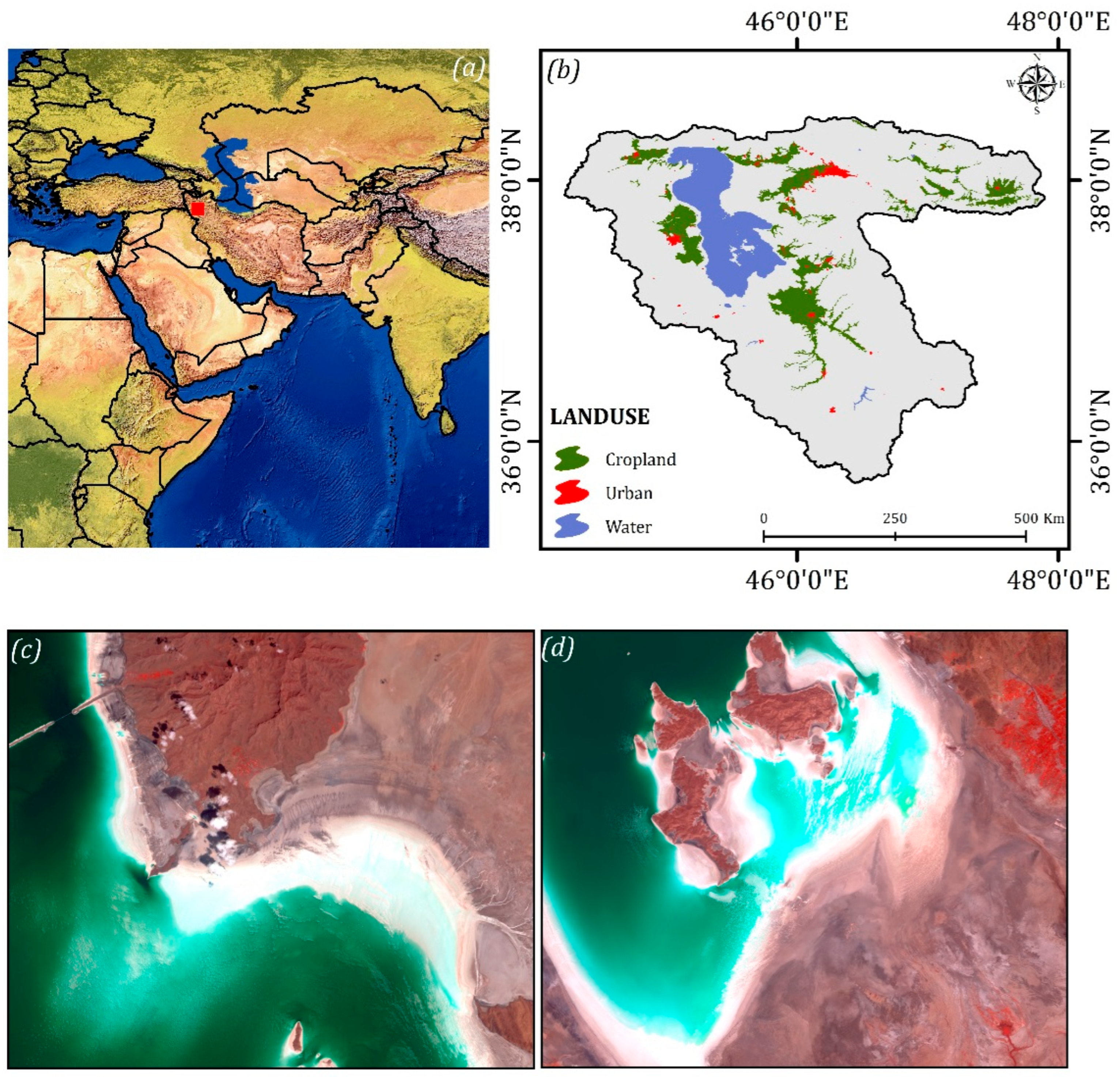
2. Location of Study Area
3. Materials and Methodology
3.1. Materials
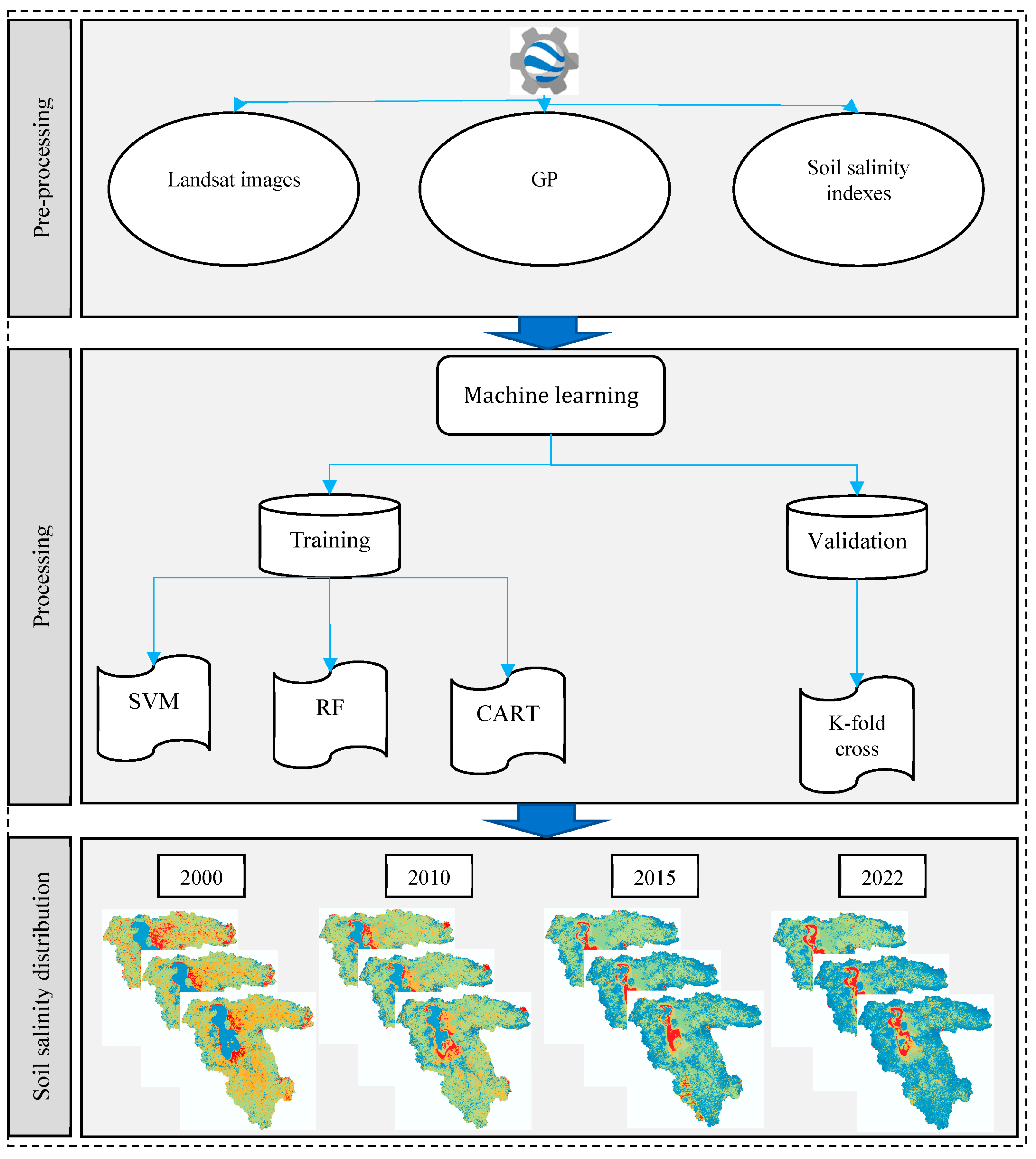
3.2. Methodology
3.2.1. Google Earth Engine
3.2.2. Support Vector Machine (SVM)
3.2.3. Random Forest (RF)
3.2.4. Classification and Regression Trees (CART)
3.3. Accuracy Assessment
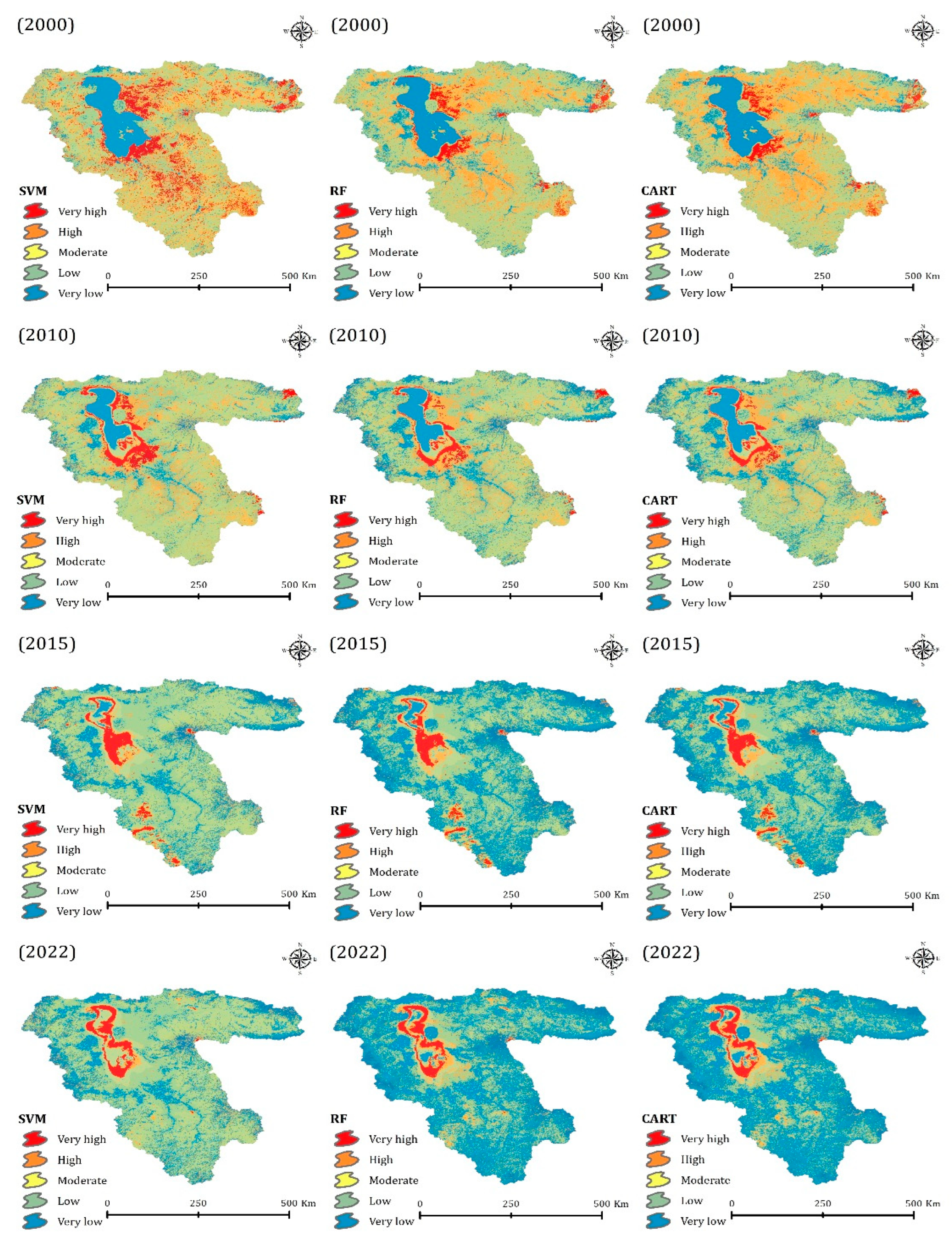
4. Results
5. Discussion
5.1. General Discussion
5.2. Probability of Saline Storm Occurrences from 2000 to 2022
5.3. Efficiency of Remote Sensing and GEE for Modeling the Probability of Saline Storm Occurrence
5.4. The Effects of Saline Storms on the Local Environment and Inhabitation
5.5. Limitation of the Present Research
6. Conclusions
Funding
Institutional Review Board Statement
Informed Consent Statement
Data Availability Statement
Conflicts of Interest
References
- Bannari, A.; Guedon, A.M.; El-Harti, A.; Cherkaoui, F.Z.; El-Ghmari, A. Characterization of slightly and moderately saline and sodic soils in irrigated agricultural land using simulated data of advanced land imaging (EO-1) sensor. Commun. Soil Sci. Plant Anal. 2008, 39, 2795–2811. [Google Scholar] [CrossRef]
- Asfaw, E.; Suryabhagavan, K.V.; Argaw, M. Soil salinity modeling and mapping using remote sensing and GIS: The case of Wonji sugar cane irrigation farm, Ethiopia. J. Saudi Soc. Agric. Sci. 2018, 17, 250–258. [Google Scholar] [CrossRef]
- Gorji, T.; Sertel, E.; Tanik, A. Monitoring soil salinity via remote sensing technology under data scarce conditions: A case study from Turkey. Ecol. Indic. 2017, 74, 384–391. [Google Scholar] [CrossRef]
- El Hafyani, M.; Essahlaoui, A.; El Baghdadi, M.; Teodoro, A.C.; Mohajane, M.; El Hmaidi, A.; El Ouali, A. Modeling and mapping of soil salinity in Tafilalet plain (Morocco). Arab. J. Geosci. 2019, 12, 35. [Google Scholar] [CrossRef]
- Kazemi Garajeh, M.; Malakyar, F.; Weng, Q.; Feizizadeh, B.; Blaschke, T.; Lakes, T. An automated deep learning convolutional neural network algorithm applied for soil salinity distribution mapping in Lake Urmia, Iran. Sci. Total Environ. 2021, 778, 146253. [Google Scholar] [CrossRef]
- Moreira, L.C.J.; Teixeira, A.D.S.; Galvão, L.S. Potential of multispectral and hyperspectral data to detect saline-exposed soils in Brazil. GIScience Remote Sens. 2015, 52, 416–436. [Google Scholar] [CrossRef]
- Ivits, E.; Cherlet, M.; Tóth, T.; Lewińska, K.E.; Tóth, G. Characterisation of productivity limitation of salt-affected lands in different climatic regions of Europe using remote sensing derived productivity indicators. Land Degrad. Dev. 2013, 24, 438–452. [Google Scholar] [CrossRef]
- Elhag, M. Evaluation of different soil salinity mapping using remote sensing techniques in arid ecosystems, Saudi Arabia. J. Sens. 2016, 2016, 7596175. [Google Scholar] [CrossRef]
- Metternicht, G.I.; Zinck, J.A. Remote sensing of soil salinity: Potentials and constraints. Remote Sens. Environ. 2003, 85, 1–20. [Google Scholar] [CrossRef]
- Taghadosi, M.M.; Hasanlou, M.; Eftekhari, K. Soil salinity mapping using dual-polarized SAR Sentinel-1 imagery. Int. J. Remote Sens. 2019, 40, 237–252. [Google Scholar] [CrossRef]
- Omrani, M.; Shahbazi, F.; Feizizadeh, B.; Oustan, S.; Najafi, N. Application of remote sensing indices to digital soil salt composition and ionic strength mapping in the east shore of Urmia Lake, Iran. Remote Sens. Appl. Soc. Environ. 2021, 22, 100498. [Google Scholar] [CrossRef]
- Yu, H.; Liu, M.; Du, B.; Wang, Z.; Hu, L.; Zhang, B. Mapping soil salinity/sodicity by using Landsat OLI imagery and PLSR algorithm over semiarid West Jilin Province, China. Sensors 2018, 18, 1048. [Google Scholar] [CrossRef] [PubMed]
- Wang, J.; Ding, J.; Yu, D.; Ma, X.; Zhang, Z.; Ge, X.; Teng, D.; Li, X.; Liang, J.; Lizaga, I.; et al. Capability of Sentinel-2 MSI data for monitoring and mapping of soil salinity in dry and wet seasons in the Ebinur Lake region, Xinjiang, China. Geoderma 2019, 353, 172–187. [Google Scholar] [CrossRef]
- Davis, E.; Wang, C.; Dow, K. Comparing Sentinel-2 MSI and Landsat 8 OLI in soil salinity detection: A case study of agricultural lands in coastal North Carolina. Int. J. Remote Sens. 2019, 40, 6134–6153. [Google Scholar] [CrossRef]
- Taghadosi, M.M.; Hasanlou, M.; Eftekhari, K. Retrieval of soil salinity from Sentinel-2 multispectral imagery. Eur. J. Remote Sens. 2019, 52, 138–154. [Google Scholar] [CrossRef]
- Nguyen, K.A.; Liou, Y.A.; Tran, H.P.; Hoang, P.P.; Nguyen, T.H. Soil salinity assessment by using near-infrared channel and Vegetation Soil Salinity Index derived from Landsat 8 OLI data: A case study in the Tra Vinh Province, Mekong Delta, Vietnam. Prog. Earth Planet. Sci. 2020, 7, 126489. [Google Scholar] [CrossRef]
- Gorji, T.; Yildirim, A.; Hamzehpour, N.; Tanik, A.; Sertel, E. Soil salinity analysis of Urmia Lake Basin using Landsat-8 OLI and Sentinel-2A based spectral indices and electrical conductivity measurements. Ecol. Indic. 2020, 112, 106173. [Google Scholar] [CrossRef]
- Khan, N.M.; Rastoskuev, V.V.; Sato, Y.; Shiozawa, S. Assessment of hydrosaline land degradation by using a simple approach of remote sensing indicators. Agric. Water Manag. 2005, 77, 96–109. [Google Scholar] [CrossRef]
- Douaoui, A.; Nicolas, H.; Walter, C. Detecting salinity hazards within a semiarid context by means of combining soil and remote-sensing data. Geoderma 2006, 134, 217–230. [Google Scholar] [CrossRef]
- Yahiaoui, I.; Douaoui, A.; Zhang, Q.; Ziane, A. Soil salinity prediction in the Lower Cheliff plain (Algeria) based on remote sensing and topographic feature analysis. J. Arid Land 2015, 7, 794–805. [Google Scholar] [CrossRef]
- Jafari, A.; Khademi, H.; Finke, P.A.; Van de Wauw, J.; Ayoubi, S. Spatial prediction of soil great groups by boosted regression trees using a limited point dataset in an arid region, southeastern Iran. Geoderma 2014, 232, 148–163. [Google Scholar] [CrossRef]
- Meier, M.; Souza, E.D.; Francelino, M.R.; Fernandes Filho, E.I.; Schaefer, C.E.G.R. Digital soil mapping using machine learning algorithms in a tropical mountainous area. Rev. Bras. Ciência Solo 2018, 42, e0170421. [Google Scholar] [CrossRef]
- Shahabi, M.; Jafarzadeh, A.A.; Neyshabouri, M.R.; Ghorbani, M.A.; Valizadeh Kamran, K. Spatial modeling of soil salinity using multiple linear regression, ordinary kriging and artificial neural network methods. Arch. Agron. Soil Sci. 2017, 63, 151–160. [Google Scholar] [CrossRef]
- Ma, S.; He, B.; Ge, X.; Luo, X. Spatial prediction of soil salinity based on the Google Earth Engine platform with multitemporal synthetic remote sensing images. Ecol. Inform. 2023, 75, 102111. [Google Scholar] [CrossRef]
- Kazemi Garajeh, M.; Laneve, G.; Rezaei, H.; Sadeghnejad, M.; Mohamadzadeh, N.; Salmani, B. Monitoring Trends of CO, NO2, SO2, and O3 Pollutants Using Time-Series Sentinel-5 Images Based on Google Earth Engine. Pollutants 2023, 3, 255–279. [Google Scholar] [CrossRef]
- Chen, S.; Woodcock, C.E.; Bullock, E.L.; Arévalo, P.; Torchinava, P.; Peng, S.; Olofsson, P. Monitoring temperate forest degradation on Google Earth Engine using Landsat time series analysis. Remote Sens. Environ. 2021, 265, 112648. [Google Scholar] [CrossRef]
- da Silva, M.V.; Pandorfi, H.; de Oliveira-Júnior, J.F.; da Silva, J.L.B.; de Almeida, G.L.P.; de Assunção Montenegro, A.A.; Mesquita, M.; Ferreira, M.B.; Santana, T.C.; Marinho, G.T.B.; et al. Remote sensing techniques via Google Earth Engine for land degradation assessment in the Brazilian semiarid region, Brazil. J. South Am. Earth Sci. 2022, 120, 104061. [Google Scholar] [CrossRef]
- Zurqani, H.A.; Post, C.J.; Mikhailova, E.A.; Schlautman, M.A.; Sharp, J.L. Geospatial analysis of land use change in the Savannah River Basin using Google Earth Engine. Int. J. Appl. Earth Obs. Geoinf. 2018, 69, 175–185. [Google Scholar] [CrossRef]
- Liang, J.; Chen, C.; Song, Y.; Sun, W.; Yang, G. Long-term mapping of land use and cover changes using Landsat images on the Google Earth Engine Cloud Platform in bay area-A case study of Hangzhou Bay, China. Sustain. Horiz. 2023, 7, 100061. [Google Scholar] [CrossRef]
- Kazemi Garajeh, M.; Salmani, B.; Zare Naghadehi, S.; Valipoori Goodarzi, H.; Khasraei, A. An integrated approach of remote sensing and geospatial analysis for modeling and predicting the impacts of climate change on food security. Sci. Rep. 2023, 13, 1057. [Google Scholar] [CrossRef]
- Aghazadeh, F.; Ghasemi, M.; Garajeh, M.K.; Feizizadeh, B.; Karimzadeh, S.; Morsali, R. An integrated approach of deep learning convolutional neural network and google earth engine for salt storm monitoring and mapping. Atmos. Pollut. Res. 2023, 14, 101689. [Google Scholar] [CrossRef]
- Kazemi Garajeh, M.; Li, Z.; Hasanlu, S.; Zare Naghadehi, S.; Hossein Haghi, V. Developing an integrated approach based on geographic object-based image analysis and convolutional neural network for volcanic and glacial landforms mapping. Sci. Rep. 2022, 12, 21396. [Google Scholar] [CrossRef]
- Feizizadeh, B.; Garajeh, M.K.; Lakes, T.; Blaschke, T. A deep learning convolutional neural network algorithm for detecting saline flow sources and mapping the environmental impacts of the Urmia Lake drought in Iran. Catena 2021, 207, 105585. [Google Scholar] [CrossRef]
- Mahdianpari, M.; Brisco, B.; Salehi, B.; Granger, J.; Mohammadimanesh, F.; Lang, M.; Toure, S. Toward a North American continental wetland map from space: Wetland classification using satellite imagery and machine learning algorithms on Google Earth Engine. In Radar Remote Sensing; Elsevier: Amsterdam, The Netherlands, 2022; pp. 357–373. [Google Scholar]
- Chen, H.; Yunus, A.P.; Nukapothula, S.; Avtar, R. Modelling Arctic coastal plain lake depths using machine learning and Google Earth Engine. Phys. Chem. Earth Parts A/B/C 2022, 126, 103138. [Google Scholar] [CrossRef]
- Waleed, M.; Sajjad, M.; Shazil, M.S.; Tariq, M.; Alam, M.T. Machine learning-based spatial-temporal assessment and change transition analysis of wetlands: An application of Google Earth Engine in Sylhet, Bangladesh (1985–2022). Ecol. Inform. 2023, 75, 102075. [Google Scholar] [CrossRef]
- Imanni, H.S.; El Harti, A.; Bachaoui, E.M.; Mouncif, H.; Eddassouqui, F.; Hasnai, M.A.; Zinelabidine, M.I. Multispectral UAV data for detection of weeds in a citrus farm using machine learning and Google Earth Engine: Case study of Morocco. Remote Sens. Appl. Soc. Environ. 2023, 30, 100941. [Google Scholar]
- Feizizadeh, B.; Omarzadeh, D.; Kazemi Garajeh, M.; Lakes, T.; Blaschke, T. Machine learning data-driven approaches for land use/cover mapping and trend analysis using Google Earth Engine. J. Environ. Plan. Manag. 2023, 66, 665–697. [Google Scholar] [CrossRef]
- Ahmadi, H.; Argany, M.; Ghanbari, A.; Ahmadi, M. Visualized spatiotemporal data mining in investigation of Urmia Lake drought effects on increasing of PM10 in Tabriz using Space-Time Cube (2004–2019). Sustain. Cities Soc. 2022, 76, 103399. [Google Scholar] [CrossRef]
- Abbasian, M.S.; Najafi, M.R.; Abrishamchi, A. Increasing risk of meteorological drought in the Lake Urmia basin under climate change: Introducing the precipitation–temperature deciles index. J. Hydrol. 2021, 592, 125586. [Google Scholar] [CrossRef]
- Amirataee, B.; Montaseri, M.; Rezaie, H. Regional analysis and derivation of copula-based drought Severity-Area-Frequency curve in Lake Urmia basin, Iran. J. Environ. Manag. 2018, 206, 134–144. [Google Scholar] [CrossRef]
- Pouladi, P.; Badiezadeh, S.; Pouladi, M.; Yousefi, P.; Farahmand, H.; Kalantari, Z.; Yu, D.J.; Sivapalan, M. Interconnected governance and social barriers impeding the restoration process of Lake Urmia. J. Hydrol. 2021, 598, 126489. [Google Scholar] [CrossRef]
- Abbas, A.; Khan, S. Using remote sensing techniques for appraisal of irrigated soil salinity. In International Congress on Modelling and Simulation (MODSIM); Modelling and Simulation Society of Australia and New Zealand: Christchurch, New Zealand, 2007; pp. 2632–2638. [Google Scholar]
- You, N.; Dong, J. Examining earliest identifiable timing of crops using all available Sentinel 1/2 imagery and Google Earth Engine. ISPRS J. Photogramm. Remote Sens. 2020, 161, 109–123. [Google Scholar] [CrossRef]
- Thieme, A.; Yadav, S.; Oddo, P.C.; Fitz, J.M.; McCartney, S.; King, L.; Keppler, J.; McCarty, G.W.; Hively, W.D. Using NASA Earth observations and Google Earth Engine to map winter cover crop conservation performance in the Chesapeake Bay watershed. Remote Sens. Environ. 2020, 248, 111943. [Google Scholar] [CrossRef]
- Sulova, A.; Jokar Arsanjani, J. Exploratory analysis of driving force of wildfires in Australia: An application of machine learning within Google Earth engine. Remote Sens. 2020, 13, 10. [Google Scholar] [CrossRef]
- Vapnik, V. The Nature of Statistical Learning Theory; Springer: New York, NY, USA, 1995. [Google Scholar]
- Chung, L.C.H.; Xie, J.; Ren, C. Improved machine-learning mapping of local climate zones in metropolitan areas using composite Earth observation data in Google Earth Engine. Build. Environ. 2021, 199, 107879. [Google Scholar] [CrossRef]
- Zhang, Q.; Xiao, J.; Tian, C.; Chun-Wei Lin, J.; Zhang, S. A robust deformed convolutional neural network (CNN) for image denoising. CAAI Trans. Intell. Technol. 2023, 8, 331–342. [Google Scholar] [CrossRef]
- Cao, J.; Zhang, Z.; Luo, Y.; Zhang, L.; Zhang, J.; Li, Z.; Tao, F. Wheat yield predictions at a county and field scale with deep learning, machine learning, and google earth engine. Eur. J. Agron. 2021, 123, 126204. [Google Scholar] [CrossRef]
- Sun, L.; Wen, J.; Wang, J.; Zhao, Y.; Zhang, B.; Wu, J.; Xu, Y. Two-view attention-guided convolutional neural network for mammographic image classification. CAAI Trans. Intell. Technol. 2023, 8, 453–467. [Google Scholar] [CrossRef]
- Tselka, I.; Detsikas, S.E.; Petropoulos, G.P.; Demertzi, I.I. Google Earth Engine and machine learning classifiers for obtaining burnt area cartography: A case study from a Mediterranean setting. In Geoinformatics for Geosciences; Elsevier: Amsterdam, The Netherlands, 2023; pp. 131–148. [Google Scholar]
- Roy, P.K.; Saumya, S.; Singh, J.P.; Banerjee, S.; Gutub, A. Analysis of community question-answering issues via machine learning and deep learning: State-of-the-art review. CAAI Trans. Intell. Technol. 2023, 8, 95–117. [Google Scholar] [CrossRef]
- Shamshiri, R.; Eide, E.; Høyland, K.V. Spatio-temporal distribution of sea-ice thickness using a machine learning approach with Google Earth Engine and Sentinel-1 GRD data. Remote Sens. Environ. 2022, 270, 112851. [Google Scholar] [CrossRef]
- Wang, X.; Wang, S.; Chen, P.Y.; Lin, X.; Chin, P. Block switching: A stochastic approach for deep learning security. arXiv 2020, arXiv:2002.07920. [Google Scholar] [CrossRef]
- Stumpf, A.; Kerle, N. Object-oriented mapping of landslides using Random Forests. Remote Sens. Environ. 2011, 115, 2564–2577. [Google Scholar] [CrossRef]
- Zhao, F.; Feng, S.; Xie, F.; Zhu, S.; Zhang, S. Extraction of long time series wetland information based on Google Earth Engine and random forest algorithm for a plateau lake basin—A case study of Dianchi Lake, Yunnan Province, China. Ecol. Indic. 2023, 146, 109813. [Google Scholar] [CrossRef]
- Suryono, H.; Kuswanto, H.; Iriawan, N. Rice phenology classification based on random forest algorithm for data imbalance using Google Earth engine. Procedia Comput. Sci. 2022, 197, 668–676. [Google Scholar] [CrossRef]
- Shakeel, N.; Shakeel, S. Context-Free Word Importance Scores for Attacking Neural Networks. J. Comput. Cogn. Eng. 2022, 1, 187–192. [Google Scholar] [CrossRef]
- Choudhuri, S.; Venkateswara, H.; Sen, A. Coupling Adversarial Learning with Selective Voting Strategy for Distribution Alignment in Partial Domain Adaptation. arXiv 2022, arXiv:2207.08145. [Google Scholar] [CrossRef]
- Aji, M.A.P.; Kamal, M.; Farda, N.M. Mangrove species mapping through phenological analysis using random forest algorithm on Google Earth Engine. Remote Sens. Appl. Soc. Environ. 2023, 30, 100978. [Google Scholar] [CrossRef]
- Bittencourt, H.R.; Clarke, R.T. Use of classification and regression trees (CART) to classify remotely-sensed digital images. In Proceedings of the 2003 IEEE International Geoscience and Remote Sensing Symposium, Toulouse, France, 21–25 July 2003; IEEE: Piscataway, NJ, USA, 2003; Volume 6, pp. 3751–3753. [Google Scholar]
- Ghosh, S.; Kumar, D.; Kumari, R. Google earth engine based computational system for the earth and environment monitoring applications during the COVID-19 pandemic using thresholding technique on SAR datasets. Phys. Chem. Earth Parts A/B/C 2022, 127, 103163. [Google Scholar] [CrossRef]
- Jia, Z.; Wang, W.; Zhang, J.; Li, H. Contact High-Temperature Strain Automatic Calibration and Precision Compensation Research. J. Artif. Intell. Technol. 2022, 2, 69–76. [Google Scholar]
- Hu, X.; Kuang, Q.; Cai, Q.; Xue, Y.; Zhou, W.; Li, Y. A Coherent Pattern Mining Algorithm Based on All Contiguous Column Bicluster. J. Artif. Intell. Technol. 2022, 2, 80–92. [Google Scholar] [CrossRef]
- Li, J.; Li, L.; Song, Y.; Chen, J.; Wang, Z.; Bao, Y.; Zhang, W.; Meng, L. A robust large-scale surface water mapping framework with high spatiotemporal resolution based on the fusion of multi-source remote sensing data. Int. J. Appl. Earth Obs. Geoinf. 2023, 118, 103288. [Google Scholar] [CrossRef]
- Bai, S.B.; Wang, J.; Lu, G.N.; Kanevski, M.; Pozdnoukhov, A. GIS-based landslide susceptibility mapping with comparisons of results from machine learning methods process versus logistic regression in Bailongjiang river basin, China. In Geophysical Research Abstracts; EGU General Assembly: Vienna, Austria, 2008; Volume 10, pp. 1–2. [Google Scholar]
- Arabameri, A.; Roy, J.; Saha, S.; Blaschke, T.; Ghorbanzadeh, O.; Tien Bui, D. Application of probabilistic and machine learning models for groundwater potentiality mapping in Damghan sedimentary plain, Iran. Remote Sens. 2019, 11, 3015. [Google Scholar] [CrossRef]
- Meng, J.; Li, Y.; Liang, H.; Ma, Y. Single-image dehazing based on two-stream convolutional neural network. J. Artif. Intell. Technol. 2022, 2, 100–110. [Google Scholar] [CrossRef]
- Ćalasan, M.; Aleem, S.H.A.; Zobaa, A.F. On the root mean square error (RMSE) calculation for parameter estimation of photovoltaic models: A novel exact analytical solution based on Lambert W function. Energy Convers. Manag. 2020, 210, 112716. [Google Scholar] [CrossRef]
- Hamzehpour, N.; Bogaert, P. Improved spatiotemporal monitoring of soil salinity using filtered kriging with measurement errors: An application to the West Urmia Lake, Iran. Geoderma 2017, 295, 22–33. [Google Scholar] [CrossRef]
- Peng, J.; Biswas, A.; Jiang, Q.; Zhao, R.; Hu, J.; Hu, B.; Shi, Z. Estimating soil salinity from remote sensing and terrain data in southern Xinjiang Province, China. Geoderma 2019, 337, 1309–1319. [Google Scholar] [CrossRef]


| Spectral Indexes | Acronym | Formula | References | R2 (2000) | R2 (2010) | R2 (2015) | R2 (2022) |
|---|---|---|---|---|---|---|---|
| Normalized difference salinity | NDSI | [18] | 0.48 | 0.66 | 0.58 | 0.63 | |
| Salinity index 1 | SI1 | [18] | 0.63 | 0.79 | 0.56 | 0.48 | |
| Salinity index 2 | SI2 | [43] | 066 | 0.68 | 0.85 | 0.88 | |
| Salinity index 3 | SI3 | [19] | 0.78 | 0.49 | 0.58 | 0.89 | |
| Salinity index I | S1 | [18] | 0.33 | 0.75 | 0.68 | 0.54 | |
| Salinity index II | S2 | [19] | 0.32 | 0.77 | 0.66 | 0.52 | |
| Salinity index III | S3 | [19] | 0.55 | 0.75 | 0.73 | 0.69 | |
| Salinity index V | S5 | [18] | 0.63 | 0.83 | 0.86 | 0.83 | |
| Salinity index VI | S6 | [18] | 0.51 | 0.22 | 0.37 | 0.52 |
| Year | SVM | RF | CART | |||
|---|---|---|---|---|---|---|
| R2 | RMSE | R2 | RMSE | R2 | RMSE | |
| 2000 | 91.12 | 4.21 | 87.36 | 5.89 | 85.65 | 6.65 |
| 2010 | 90.45 | 4.89 | 86.78 | 6.42 | 85.11 | 6.87 |
| 2015 | 91.78 | 3.99 | 87.12 | 6.24 | 84.99 | 7.12 |
| 2022 | 91.65 | 4.09 | 87.01 | 6.13 | 85.21 | 6.94 |
| 2000 | 2010 | ||||||
|---|---|---|---|---|---|---|---|
| Class | SVM | RF | CART | Class | SVM | RF | CART |
| Very low | 12.00 | 16.20 | 16.22 | Very low | 12.93 | 21.42 | 23.79 |
| Low | 47.47 | 56.88 | 47.20 | Low | 66.10 | 60.92 | 58.55 |
| Moderate | 29.93 | 23.88 | 33.54 | Moderate | 16.17 | 14.50 | 14.65 |
| High | 9.54 | 2.12 | 2.12 | High | 3.71 | 2.00 | 1.76 |
| Very high | 1.07 | 0.92 | 0.92 | Very high | 1.09 | 1.17 | 1.26 |
| 2015 | 2022 | ||||||
| Class | SVM | RF | CART | Class | SVM | RF | CART |
| Very low | 26.64 | 50.38 | 49.07 | Very low | 28.53 | 62.21 | 65.96 |
| Low | 67.08 | 43.02 | 44.33 | Low | 66.35 | 30.60 | 26.85 |
| Moderate | 2.51 | 3.29 | 3.30 | Moderate | 1.97 | 4.30 | 4.30 |
| High | 2.44 | 1.60 | 1.59 | High | 1.86 | 1.58 | 1.58 |
| Very high | 1.33 | 1.70 | 1.70 | Very high | 1.29 | 1.32 | 1.32 |
| Product Name | 2000 | 2010 | 2015 | 2022 |
|---|---|---|---|---|
| AOD thickness | 0.285 | 0.416 | 0.423 | 0.459 |
| Methods | SVM | RF | CART |
|---|---|---|---|
| R2 | 0.69 | 0.69 | 0.73 |
Disclaimer/Publisher’s Note: The statements, opinions and data contained in all publications are solely those of the individual author(s) and contributor(s) and not of MDPI and/or the editor(s). MDPI and/or the editor(s) disclaim responsibility for any injury to people or property resulting from any ideas, methods, instructions or products referred to in the content. |
© 2024 by the author. Licensee MDPI, Basel, Switzerland. This article is an open access article distributed under the terms and conditions of the Creative Commons Attribution (CC BY) license (https://creativecommons.org/licenses/by/4.0/).
Share and Cite
Kazemi Garajeh, M. Monitoring the Spatio-Temporal Distribution of Soil Salinity Using Google Earth Engine for Detecting the Saline Areas Susceptible to Salt Storm Occurrence. Pollutants 2024, 4, 1-15. https://doi.org/10.3390/pollutants4010001
Kazemi Garajeh M. Monitoring the Spatio-Temporal Distribution of Soil Salinity Using Google Earth Engine for Detecting the Saline Areas Susceptible to Salt Storm Occurrence. Pollutants. 2024; 4(1):1-15. https://doi.org/10.3390/pollutants4010001
Chicago/Turabian StyleKazemi Garajeh, Mohammad. 2024. "Monitoring the Spatio-Temporal Distribution of Soil Salinity Using Google Earth Engine for Detecting the Saline Areas Susceptible to Salt Storm Occurrence" Pollutants 4, no. 1: 1-15. https://doi.org/10.3390/pollutants4010001