Numerical Simulation of Dispersion Patterns and Air Emissions for Optimal Location of New Industries Accounting for Environmental Risks

Abstract

One of the main reasons for air pollution is industrial plants releasing huge amounts of air pollutants in the form of gas emissions. The different chemical pollutants and their corresponding levels present in these emissions, and their proximity to the industrial source, have serious effects on the nearby ecosystems. Some of the industrial nuisances include noise, smoke, dirt, dust, odor and noxious gases, which have to be minimized (if possible, eliminated), especially if the location is desired to be used as a community site. When choosing locations at which to build either new industrial plants or new community sites, software can be used to assess both the short-term and long-term concentration profiles of the various detrimental air pollutants. In this study, the AERMOD model was used to find an optimal location to build a new plant in Toledo, Ohio, USA. Simulations were performed to study the pollutant emissions and their dispersion patterns for four different geographic locations situated away from an existing plant in this region. The AERMOD model, along with the IRAP-h View model, which is approved by the US Environmental Protection Agency (EPA), has been successfully used to assess the fate and transport of pollutants from the proposed new industrial plants. The hazard quotients from the analysis of the results for these four different geographic locations were assessed. The highest total non-cancer hazard indices of 18.7 and 13.2 were obtained for fisher adult and fisher child, respectively, in one of the four locations. The acute inhalation quotient risk was less than the target hazard index of 0.25 for all the four locations. With respect to the concentrations of several chemicals of potential concern (COPC), such as soil, produce, beef, chicken, milk and pork, the fourth location (farthest east) recorded the minimum range values compared to the other three locations.

1. Introduction

Among the different types of pollution, gas emissions originating from industrial sources can be considered as a major source of air pollution. Pollutants in these emissions have a major impact on the ecosystems close to the industrial sources. Some of the common air pollutants include gases (e.g., SO_x, NO_x, CO, HC_s, volatile organic compounds, etc.), particulate matter (e.g., smoke, dust, ash, fumes, aerosols, pollen), radioactive materials and many others. Industrial activities, such as oil refining, the production of specialty chemicals, fertilizers, organic and inorganic chemicals and power generation, contribute to a significant share of the overall air pollution. Study of the dispersion of these air pollutants into the air, water and soil is important not only for the planning of new premises for communities but also for building new industrial plants. The detrimental effects of pollutant gases that are emitted due to air pollution are due to a chain of different events, such as the formation of air pollutants in a process, to their emission, chemical transformation, dispersion into the atmosphere, uptake by a receptor and health effects.

Dispersion modeling is most often used by companies to construct or modify an industrial facility, and it is also useful for emergency planning and capital planning. The main application of air dispersion modeling is to review air quality scenarios so that the associated environmental impact on the area of study can be quantified and predicted [1,2,3,4,5]. Some of the advantages of using air dispersion models include managing existing emission rates, planning new facilities, the calculation of the optimal stack height, measuring the risks and preparing for emergency situations and comparing and evaluating the influence of air quality, standards, criteria and guidelines with existing emission rates. The aim of the current study is to assess the potential impacts associated with the emissions of toxic air contaminants from a new industrial location in order to select the best location for a new industrial plant based on human health risk assessment. Firstly, the gas emissions of all significant sources in an industrial complex (taken as a case study) are estimated, and then the pollutant concentrations and distributions in the industrial complex area are assessed and estimated by using the American Meteorological Society–Environmental Protection Agency Regulatory Model (AERMOD). The AERMOD model has been successfully used for predicting the emissions of various pollutants originating from different sources. This model is widely used for studying emissions in the US and Europe and has potential to be used for applications in Asia too [6,7,8,9]. AERMOD has also been used to study several pollutants that include hydrogen cyanide, sulfur hexafluoride, VOCs, the dispersion of heavy metals and total gaseous mercury [10,11,12,13]. The use of AERMOD for heavy metal dispersion is more efficient compared to a thorough experimental analysis of the samples for a larger area of investigation, as this would be tedious and time-consuming [14]. Depending on the area of investigation (country), AERMOD is coupled with local weather research and forecasting, whose output parameters, such as temperature, wind speed and wind direction, are also evaluated [15]. There are other models, such as MODELAR (Modelo Regulatório de Qualidade do Ar), ADMS-Urban, CALPUFF and SCREEN3, similar to AERMOD, that are used to study the dispersion of air pollutants [16,17,18,19].

In the present study, the main objective is to find an optimal location for a new industrial plant based on the pollutant propagation predictions obtained from simulations. In order to compare the acceptable risk levels to exposure information (either measured or calculated) and to predict potential risks with safety factors, the Industrial Risk Industrial Program—Human Health (IRAP-h) View software package (based on the United States Environment Protection Agency (USEPA)) is used to evaluate potential locations for a new industrial plant. Reference concentrations and acceptable risk levels are employed based on the scientific evidence available. Four main components are analyzed: receptor identification; hazard identification; exposure assessment; and risk characterization. In addition, the AERMOD is used for the prediction of the maximum health impacts and deposition rates in the proposed locations. In Section 2, the details of the AERMOD model are described, along with the parameters used in the simulations. Section 2 also includes a brief description of the procedure for the estimation of the pollutant exposure levels, exposure level scenario and location selection. Section 3 gives more details on the quantification of cancer risk and cancer hazards. In Section 4, the results obtained from these simulations are discussed and the most optimal location among the four locations is proposed.

2. Materials and Methods

2.1. AERMOD Dispersion Model

The input data used in this model are topographical data, meteorological data, dimensions of the stack and buildings around the stack, emission rate, plume temperature and pollutant specification. AERMOD is a steady-state plume model designed to calculate the near-field (less than 50 km) concentration and run with minimum observed meteorological parameters. This model is a system with three separate components: AERMOD (Aermic Dispersion Model), AERMET (AERMOD Meteorological Preprocessor) and AERMAP (AERMOD Terrain Preprocessor). AERMOD input data are prepared from output files from the AERMET and AERMAP preprocessors [20]. The AERMET program is a meteorological data preprocessor that accepts surface meteorological data, upper air soundings or data from on-site instrument towers, and then it calculates the atmospheric parameters needed by the dispersion model. Hourly surface data (Samson surface met data format) and upper air data (TD 6201 format) are obtained from elsewhere [21]. The AERMAP preprocessor calculates a representative terrain-influence height associated with each receptor by using gridded terrain data for the area of study. In this study, analysis of the three-kilometer area around the meteorological site using 12 pie-shaped sectors was used to calculate the land use parameters. For each sector, surface parameters, namely Albedo, Bowen ratio and surface roughness, were specified by the sectors that were not less than a 30-degree arc. The value of anemometer height was taken as 21 ft (6.4 m). The AERMET model was run on a short regional domain extending westward to 83.75-degree longitude and northward to 42.96-degree latitude. In this study, the AERMAP was run using two separate 1-degree Digital Elevation Models (DEMs), Toledo East and Toledo West, to cover the area of concern. The geographical data, including land use and terrain, were obtained from the Geographic Information System Resource website (www.webgis.com, accessed on 1 March 2021).

Table 1. List of United States Geological Survey (USGS) DEM 1-degree files used for AERMAP run.

Name	Half	Min	Max	Min	Max
		Longitude	Longitude	Latitude	Latitude
Toledo	West	−84°00′00″	−83°00′00″	41°00′00″	42°00′00″
Toledo	East	−83°00′00″	−82°00′00″	41°00′00″	42°00′00″

shows the details of the DEM files. The AERMAP was run using the NAD27 datum (North American Datum of 1927). These two files were used for all AERMOD runs.

2.2. Air Dispersion and Deposition Modeling

2.2.1. Control Pathway

The control pathway contains options that effectively control the AERMOD dispersion model to predict impacts based on several options, such as dispersion options, averaging time options and terrain options (elevated). In the control pathway, the overall control options are specified for both pollutants, sulfur dioxide (SO₂) and mercury (Hg). These options include dispersion options, where concentration, dry deposition, wet deposition, and total deposition were selected. The AERMOD dispersion model was run for a short-term averaging time period option (1-h) and long-term averaging time period option (annual) in order to calculate the human health risk. The human health risk assessment was performed based on the maximum 1-h average concentrations over the 3-year period. According to US EPA recommendations, the urban dispersion coefficient and mixing are recommended when the area of study is greater than 50%; otherwise, the rural coefficient and mixing heights will be applied. In this study, based on the land use for the evaluation of the study area, the dispersion coefficient was taken for the urban area for the existing plant, and as an input, an urban population of 436,393 (years 1990–1992) was used for Lucas. In addition, the dispersion environment was classified as rural for the proposed plant locations. The elevated terrain height option was used for this study.

2.2.2. Source Pathway

In the source pathway, the source input parameters and source group information, such as source type, building downwash and variable emissions, were specified. AERMOD air modeling was performed based on a unit emission rate of 1.0 g/s, instead of compound-specific emission rates. The unitized air modeling outputs based on a unit emission rate were multiplied by a compound-specific emission rate prior to use in the risk assessment. The AERMOD dispersion model was run for the periods 1990, 1991 and 1992 by using base emission inventories. Gas and particle information is required by AERMOD in order to conduct the human health risk assessment. This information includes mercury vapor, vapor, particle and particle-bound chemicals of potential concern (COPC)_s. Some chemical-specific values for the diffusivity of COPC in air and water, cuticular resistance and Henry’s law constant (HLC) are required by the AERMOD model in order to model vapor dispersion and deposition.

Table 2. Source parameters for gas and particle deposition for mercury.

Source Parameter	Mercury
Diffusivity in air (cm2/s)	1.09 × 10−2
Diffusivity in water (cm2/s)	3.01 × 10−52
Cuticular resistance (s/cm)	1.00 × 105
Henry’s law constant (Pa·m3/mol)	7.19 × 102

lists the source parameters for gas and particle deposition for mercury entered into AERMOD. The AERMOD model requires the input of particle size distribution and density data for completion of the particle phase and particle-bound phase modeling.

Table 3. Particle size distribution values.

Particle	Method	Particle Diameter (Microns)	Mass Fraction	Particle Density (g/cm3)
Particle dry	Method 1: 10% or more has a diameter ≥10 microns	2.5	0.450	1
		10	0.550	1
Particle-bounddry	Method 1: 10% or more has a diameter ≥10 microns	2.5	0.766	1
		10	0.234	1

lists the assumed values for particle size distribution, which is used as an input to the AERMOD model. Discrete Cartesian grid receptor monitoring networks were utilized for the area of study. In order to predict the concentration and depositions at Lucas County, two monitoring stations were used for the existing plant and every proposed location. The meteorological data files generated by the AERMET preprocessor for sulfur dioxide and mercury were utilized for the running of AERMOD. Wind speed was taken from model default values. For Lucas County, the average base elevation 180 m above mean sea level (MSL) was taken. The averaging results were obtained for short-term, 1-h and annual time period options.

2.3. IRAP-h Model

The IRAP-h View applied in this study is designed to accept output files of annual average concentrations and annual average deposition rates from the AERMOD dispersion model. The annual average concentration is the mean concentration over a year to which a receptor may be exposed at ground level. The annual average deposition rate is the average transfer of air pollutants from the air to ground surfaces. The IRAP-h View uses these output files to predict human exposure to pollutants emitted into the environment from the existing and proposed plants. In addition, IRAP-h View uses risk output files processed by the Risk Mode post-processor in the AERMOD software. The human health risk assessment (HHRA) is required in this study because the mercury emissions emitted from the proposed plant cannot be evaluated in terms of their effects on human health simply with reference to the National Ambient Air Quality Standards (NAAQS). In addition, mercury has appreciable potential to accumulate in the environment to harmful concentrations that could affect humans and other ecosystems. The human health risk assessment process is based on the application of the US EPA Human Health Risk Assessment Protocol (HHRAP). IRAP-h View software has been used for assessing health risks arising from exposure to air pollutants emitted by existing and proposed industrial plants. The Mercury Study Report to Congress [22] reported that there are three forms of mercury in the environment: elemental, divalent and methylated. Total mercury consists entirely of 60% elemental vapor phase, 30% divalent vapor phase and 10% divalent particle bound phase [23].

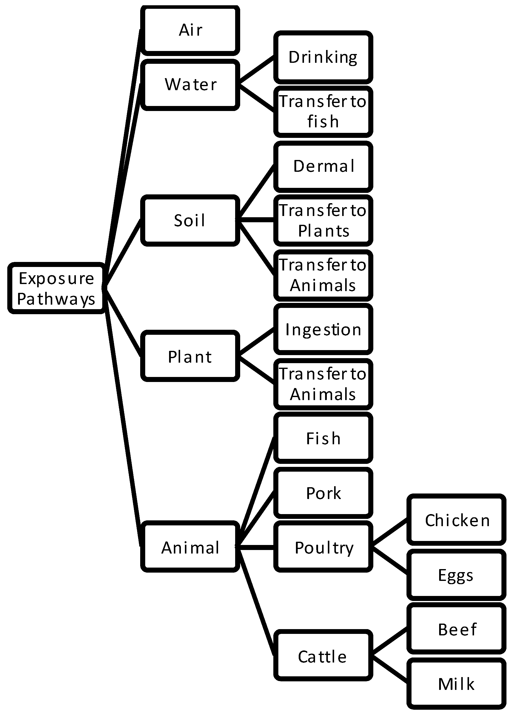
2.4. Methodology for Estimating Exposure to Emissions

Exposure to mercury occurs when the exposure pathway from the source to receptors is completed. Exposure to mercury or other COPCs can occur through direct or indirect exposure pathways. Exposure to mercury can be evaluated using different exposure pathways. The inhalation pathway is used to evaluate the exposure to elemental mercury. Direct and indirect exposure pathways both are used to evaluate the exposure to divalent mercury. Since methyl-mercury is the most toxic form of mercury, only indirect exposure pathways can be used to evaluate the exposure to methyl-mercury (CH₃Hg⁺). In order to perform a health risk assessment, both direct and indirect pathways are used in the present analysis (Figure 1).

2.5. Exposure Scenario Selection

Exposure scenarios are identified to predict the potential health impacts of the proposed industrial plants on the surrounding area. Each exposure scenario defines a particular combination of exposure pathways and the parameter values used to characterize risks and hazards. Since the area of study is located in rural, urban, grassland and water (fresh and sea) areas, seven exposure scenarios were selected for health risk assessment. The seven scenarios are: resident adult, resident child, farmer adult, farmer child, fisher adult, fisher child and acute risk. The exposure scenarios were selected based on an evaluation of the proposed land uses of the area surrounding the proposed industrial plant. The locations of exposure scenarios were the grid nodes (i.e., the actual geographic positions) at which the receptor exposure scenarios were evaluated individually. The locations of exposure scenarios were selected based on the air concentrations and deposition fluxes estimated by AERMOD and land uses within the area of concern. Proposed locations were eliminated as a parameter used to define exposure scenarios by utilizing the maximum off-site impact (based on air dispersion modeling) of all receptors in the evaluated off-property assessment area. This technique effectively maximizes the estimated exposure to every individual regardless of the actual location of the resident/farmer/fisher. Receptor polygons were drawn around each land use area of interest within the area of concern. To estimate the grid nodes within each polygon, the IRAP-h View receptor identification tool was used. These grid nodes were estimated by IRAP-h View, where the utilized air concentrations and depositions were maximized. Mercury emission rates were entered into IRAP-h View in order to estimate the single grid node. At all of these grid nodes identified by IRAP-h View, cancer risks and non-cancer risks and hazards were predicted.

Table 4. Selected exposure scenarios and associated exposure pathways considered in the present analysis.

Exposure Pathways	Exposure Scenarios
	Farmer	Farmer Child	Adult Resident	Child Resident	Fisher	Fisher Child	Acute Risk a
Inhalation of vapors and particulates	X	X	X	X	X	X	X
Incidental ingestion of soil	X	X	X	X	X	X
Ingestion of homegrown produce	X	X	X	X	X	X
Ingestion of homegrown beef	X	X
Ingestion of milk from homegrown cows	X	X
Ingestion of homegrown chicken	X	X
Ingestion of eggs from homegrown chickens	X	X
Ingestion of homegrown pork	X	X
Ingestion of fish					X	X
Ingestion of breast milk b	X		X		X

^aThe acute risk scenario evaluates short-term 1-h maximum pollutant air concentrations based on hourly emission rates.^bCOPC estimated concentrations in the three exposure scenarios indicated are utilized to model exposure to infants. Infant exposure to COPC via the ingestion of their mother’s breast milk is evaluated as an additional exposure pathway, separately from the recommended exposure scenario.

presents the chronic and acute exposure pathways and exposure scenarios considered in this study. Acute exposure was evaluated for residents only.

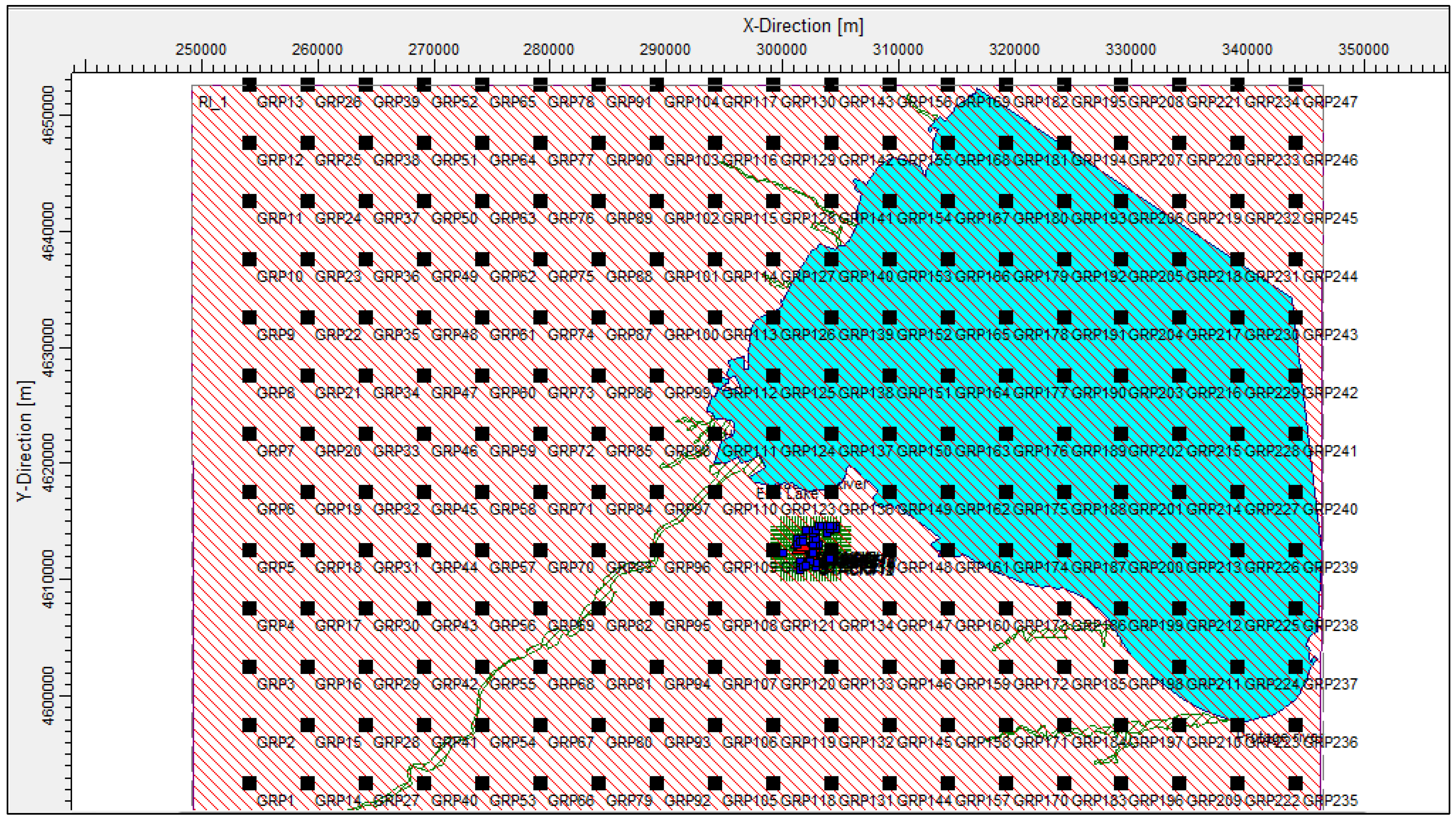
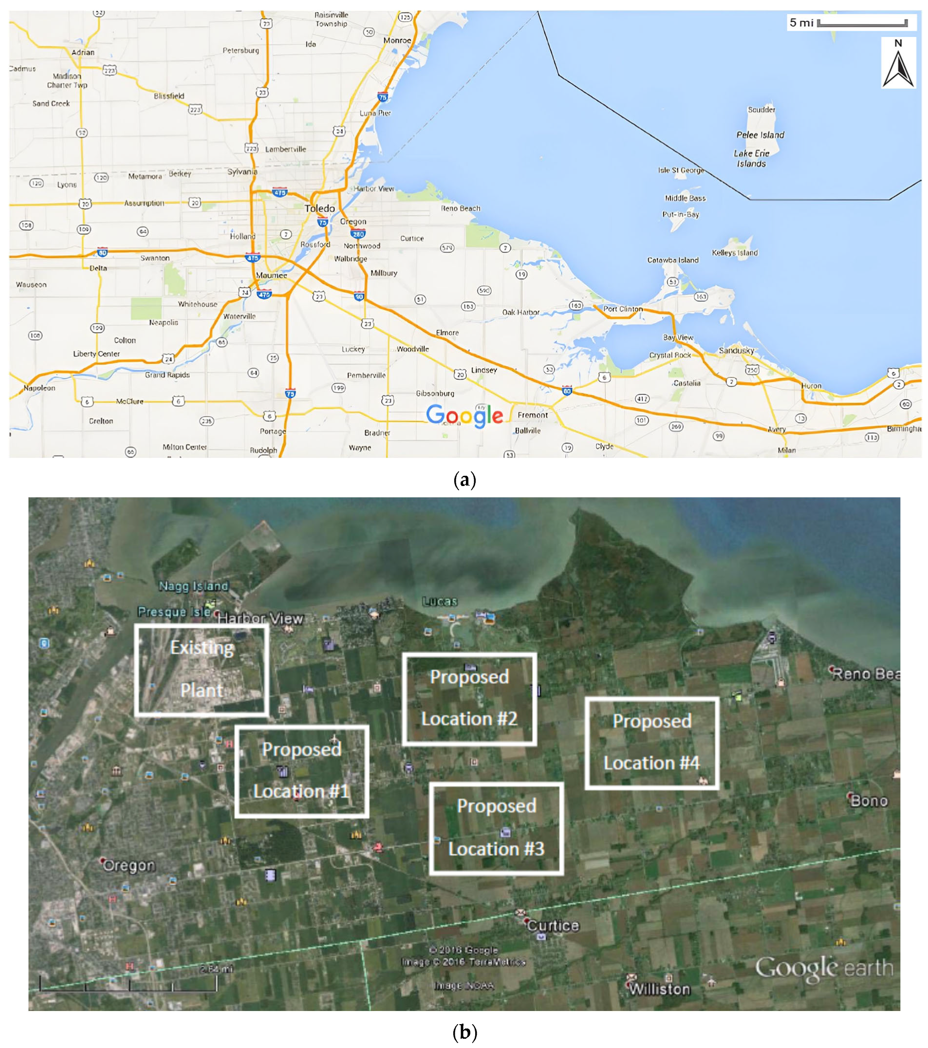
2.6. Exposure Scenario Locations

The current and reasonable potential future land use surrounding the proposed plants is considered when evaluating the potential risk. The locations associated with the exposure scenarios include occupational, residential and sensitive receptors. Sensitive receptors include community centers, hospitals, nursing homes/retirement homes, schools and day-care centers. In this study, receptor grids equal to 264 receptor locations are used for the risk assessment around every proposed plant location. The receptor locations are automatically identified by IRAP every 5000 m as a worst-case scenario, as shown in Figure 2.

2.7. Water Bodies and Watersheds

Water bodies and watersheds were selected for evaluation in order to estimate mercury concentrations in surface water and sediment. These water bodies and watersheds were drawn in IRAP-h View by drawing receptor polygons around the corresponding water bodies. The geographic information system (GIS) shape files were imported into IRAP-h View as the base map in order to define water bodies, watersheds and receptors. In this study, one water body—Lake Erie—and nine watersheds—Maumee River, Portage River, Raisin River, Toussaint River, Ottawa River, Halfway Creek, Plume Creek, Otter Creek and Swan Creek—are considered. The exposure to mercury emissions from the proposed industrial plants that are deposited on surface water bodies used for drinking purposes is considered by the drinking water ingestion pathway. The contributions from deposition onto surface water are considered by the HHRAP equations used to estimate COPC concentrations in the surface water. Lake Erie was used as a water body receptor in order to model the drinking water ingestion pathway. The Lake Erie water body and watershed polygons are shown in Figure 3a, while Figure 3b shows the graphic representation of the four proposed plants. The deposition into the fishable water bodies located near the proposed industrial plant is considered in order to model the fish ingestion pathway. Both cancer risks and non-cancer hazards from the fish ingestion pathway, calculated by considering deposition onto Lake Erie, were added.

2.8. Estimating Media Concentrations

In this study, a portion of the receptor diet is assumed to consist of produce that is either below ground or aboveground, protected or unprotected. The sum of the contamination resulting from the above three mechanisms was used to estimate the concentration of COPCs in aboveground and unprotected produce. The concentration of aboveground produce due to direct deposition (Pd) in mg of COPC per kg of DW is estimated by using Equation (1).

$$Pd=\frac{1000\ast Q\ast \left(1-F_V\right)\ast \left[Dydp+F_W\ast Dywp\right]\ast Rp\ast [1-\exp \left(-kp\ast Tp\right]}{Yp\ast kp}$$

(1)

where Q is the emission rate of COPC in g/s; F_v is the COPC air concentration fraction in the vapor phase (unitless); Dydp is the unitized yearly wet deposition from the particle phase (s/m²·year); Fw is 0.6 for cations and most organics and 0.2 for onions (unitless); Dywp is the unitized yearly wet deposition from the particle phase (s/m²·year); Rp is the interception fraction of the edible portion of a plant (unitless); kp is the plant surface loss coefficient (year⁻¹); Tp is the plant exposure length to deposition per harvest of the edible portion of the ith plant group (year); and Yp is the yield or standing crop biomass of the edible portion of the plant (productivity) (kg DW/m²).

The COPC concentration in the plant resulting from air to plant transfer Pv (µg COPC/g DW) is estimated by using Equation (2).

$$Pv=Q\ast F_V\frac{C_{yv}B{v}_{av}V{G}_{ag}}{{\rho }_a}$$

(2)

where C_yv is the unitized yearly average air concentration from the vapor phase (µg·s/g·m³); Bv_ag is the air to plant bio-transfer factor of COPC ([mg COPC/g DW plant]/[mg COPC/g air]) (unitless); VG_ag is the aboveground produce empirical correction factor (unitless); ρ_a is the air density (g/m³). The COPC concentrations in the produce due to root uptake, Pr (mg/kg), for protected produce—exposed above the ground and below the ground—are estimated by using Equations (3) and (4), respectively.

$$Pr=Cs\ast Br$$

(3)

$$Pr=\frac{Cs\ast RCF\ast V{G}_{rootveg}}{K{d}_s}$$

(4)

where Cs is the average concentration of soil over the exposure duration (mg COPC/kg soil); Br is the bio-concentration factor of plant–soil for produce (unitless); RCF is the concentration factor of roots (unitless); VG_rootveg is the empirical correction factor for belowground produce (unitless), and Kd_s is the partition coefficient of soil/water (L/kg).

The cumulative soil concentration (Cs) with carcinogenic COPCs is calculated using Equations (5) and (6), while, for non-carcinogens, Equation (7) is used.

For carcinogens, if T₂ ≤ tD then

$$Cs=\frac{Ds}{ks\ast \left(td-T_1\right)}\ast \left[\left(tD+\frac{\exp \left(-ks\ast tD\right)}{ks}\right)-\left(T_1+\frac{\exp \left(-ks\ast T_1\right)}{ks}\right)\right]$$

(5)

and if T₁ < tD < T₂, then

$$Cs=\frac{\left(\frac{Ds\ast tD-C{s}_{tD}}{ks}\right)+\left(\frac{C{s}_{td}}{ks}\right)\ast [1-\exp \left(-ks\ast \left(T_2-tD\right)\right]}{T_2-T_1}$$

(6)

$$C{s}_{tD}=\frac{Ds\ast \left[1-\exp \left(-ks\ast tD\right)\right]}{ks}$$

(7)

where Ds is the deposition term (mg COPC/kg soil/year); ks is the soil loss constant of COPC due to all processes (year⁻¹); tD is the time period over which deposition occurs (time period of combustion) (year); T₁ is the time period at the beginning of combustion (year); Cs_tD is the concentration of soil at time tD (mg/kg); T₂ is the length of exposure duration (year). Site-specific data as given in

Table 5. Site-specific data used in IRAP-h View model.

Site-Specific Parameters	Value	Unit
Average annual runoff	73.25	cm/year
Average annual precipitation	86.97	cm/year
Average annual irrigation	0	cm/year
Average annual evapotranspiration	86.36	cm/year
USLE Rainfall Factor	100	(year−1)
Depth of water column	18.90	m
Average volumetric flow rate through water body	175 × 109	m3/year
USLE Cover and Management Factor	0.10	unitless

were obtained for evapotranspiration, irrigation, runoff, watershed area and impervious watershed area, depth of water bodies, rainfall factor and volumetric flow of water bodies.

The COPC concentrations in beef, cow’s milk, pork and chicken or eggs are estimated using Equation (8).

$$A_x=\left(\sum \left(F_i·Q{p}_i·P_i\right)+\left(Q_S{C}_S{B}_S\right)\right)B{a}_X·MF$$

(8)

where A is the concentration of the COPC in x expressed in mg COPC/kg FW tissue; x is beef, cow’s milk, pork and chicken or eggs, respectively; F_i is the plant type i fraction grown on contaminated soil and ingested by the animal (x); Qp_i is the plant type i quantity eaten by the animal (x) per day (kg DW plant/day); P_i is the COPC concentration in each plant type i eaten by the animal (x) (mg/ kg DW); Q_s is the soil quantity eaten by animal (x) each day (kg/day); C_s is the average soil concentration over the exposure duration (mg COPC/kg soil); Bs is the bio-availability factor of soil (unitless); Ba_x is the bio-transfer factor of COPC for x (day/kg FW tissue); and MF is the metabolism factor (unitless).

The concentrations of COPC in fish can be calculated using a bio-accumulation factor (BAF), a bio-concentration factor (BCF) or a biota–sediment accumulation factor (BSAF). Generally, COPC concentrations in fish can be calculated using two methods. In the first method, for COPCs with a log octanol–water partitioning coefficient (K_ow) > 4, it can be estimated by multiplying a chemical-specific bio-accumulation factor by the dissolved phase water concentration. In the second method, for COPCs with a log K_ow < 4, it can be estimated by multiplying a chemical-specific bio-concentration factor by the dissolved phase water concentration. The COPC concentration sorbed to bed sediment (C_sb), used to estimate the concentration of COPC in fish, can be calculated by using Equation (9).

$$C_{sb}=f_{bs}{C}_{wtot}\left(\frac{K{d}_{bs}}{{\theta }_{bs}+K{d}_{bs}{C}_{bs}}\right)·\left(\frac{d_{wc}+d_{bs}}{d_{bs}}\right)$$

(9)

where C_sb is the concentration of COPC sorbed to bed sediment (mg COPC/ kg sediment); f_bs is the fraction of total water body COPC concentration in benthic sediment (unitless); C_wtot is the total water body COPC concentration (mg COPC/L water body); Kd_bs is the bed sediment/sediment pore water partition coefficient (L COPC/kg water body); θ_bs is the porosity of bed sediment; C_BS is the concentration of bed sediment; d_wc is the depth of the water column (m); d_bs is the depth of the upper benthic sediment layer (m).

2.9. Quantification of Exposure

The COPC concentrations in environmental exposure media and human receptor-specific exposure parameter values were combined in order to evaluate the potential for human exposure. The potential impacts of chronic exposure through direct inhalation of vapor and particulate COPCs on human health, as well as the environment, were considered for all receptors. The values of specific-toxicity chemicals were used for individual cancer risk and non-cancer hazard resulting from concentrations of COPC in air. This methodology does not account for time spent indoors, where particulates are more likely not be inhaled and to settle out or for time spent away from the maximum air concentration point. The chemical intake through ingestion can be estimated by using Equation (10) [24].

$$I=\frac{C·IR·EF·ED}{BW·AT}$$

(10)

where I is the intake (mg/kg·day); C is the concentration of COPC in the medium of concern; IR is the ingestion rate; EF is the exposure frequency (day/year); ED is the exposure duration (years); BW is the body weight (kg); and AT is the average time (days).

Animals and plants within the area of concern may deposit onto the Earth’s surface or take up COPCs in the air. The food ingestion pathways consider the potential for human exposure to COPCs. These COPCs have bio-accumulated in locally raised beef, locally grown produce, locally raised chicken, eggs and pork, milk from dairy cows and locally caught fish. There are some factors that influence human exposure through food ingestion. These factors include the food consumption rate, diet, the COPC media concentrations and the percentage of the diet that is influenced by COPC emissions from the existing and proposed plants. The concentration of COPC in the soil varied with distance from the existing and proposed sources based on air dispersion modeling and the deposition of COPCs. The potential for human exposure to COPCs, which is primarily from hand-to-mouth behavior, was considered for the soil ingestion pathway. Human exposure through soil ingestion was influenced by some factors. These factors include the rate of soil ingestion over the exposure time, soil COPC concentrations and the exposure frequency and duration. The potential for human exposure to COPCs from the ingestion of drinking water was considered for the drinking water ingestion pathway. A surface water body that may receive emissions deposition from existing and proposed plants was the main source of drinking water in this study. Human exposure via surface water ingestion was influenced by some factors. These factors include the water consumption rate, the exposure frequency and duration and the estimated COPC concentrations in the surface water. Exposure from groundwater sources used as drinking water was not evaluated since it is generally an insignificant pathway. The exposure frequency used was 350 days/year. The assumed duration of exposure to the modeled concentrations of COPCs varied based on age and the exposure pathway. Additionally, the operating life of the facility being evaluated must be considered in risk calculations. The adult chronic exposure scenarios were based on the assumption that an adult is located at the location of maximum impact continuously for the entire exposure duration. For adult farmers, the direct exposure to emissions by inhalation occurs for the anticipated operating life of the facility, but indirect exposure from the ingestion of home-grown produce and livestock continues for 40 years. Each exposure scenario receives indirect exposure through the ingestion of contaminated homegrown food and direct contact with soil and water. Chronic exposure scenarios for all children in the assessment area are based on the assumption that a child resides at the location of maximum impact from the second through the sixth year of life. During this time, the child also receives indirect exposure to the same pathways as described for adults and contaminated homegrown food. The same considerations for exposure apply to infants for the first year of life. Infants in the assessment area are assumed to be exposed to COPCs through breast milk, the inhalation pathway and the consumption of home-grown food. The HHRAP recommends the exposure duration values presented in

Table 6. Values of exposure duration.

Recommended Exposure Scenario Receptor	Value	Source
Child resident	6 years	US EPA 1990f, 1994r
Adult resident	30 years	US EPA 1990f, 1994r
Fisher	30 years	US EPA 1990f, 1994r
Fisher child	6 years	Assumed to be the same as the child resident
Farmer	40 years	US EPA 1994l, 1994r
Farmer child	6 years	Assumed to be the same as the child resident

.

3. Quantification of Cancer Risk and Non-Cancer Hazard

The carcinogenic risk is estimated as the probability of an individual developing cancer over a lifetime as a result of exposure to specified emissions. In this study, carcinogenic risk was estimated as an incremental probability of fatal cancer from exposure to emissions from each proposed plant. The potential for cancer risk caused by inhalation exposure was calculated by multiplying a chemical-specific unit risk factor by the annual average air concentration. Individual cancer risk from inhalation exposure was calculated by using Equation (11).

$$Cancer Risk=C_a\times URF$$

(11)

where C_a is the annual average concentration of COPC in air (g/m³); and URF is the unit risk factor (g/m³)⁻¹.

The potential for cancer risk caused by indirect exposure pathways was calculated by multiplying the chemical-specific cancer slope factor by the estimated lifetime average daily dose. For COPCs with non-carcinogenic effects, the potential for non-carcinogenic toxic effects in an individual is evaluated by comparing the estimated exposure level over a specified time period with the appropriate non-cancer reference dose. Both direct and indirect exposures are considered in the estimation of non-cancer health effects. In this study, the annual average concentration of COPC in the air was compared to a chronic reference concentration, and the maximum 1-h concentration was also compared to an acute inhalation exposure criterion in order to evaluate the potential for non-cancer health effects associated with inhalation exposure to the COPCs. The potential for non-cancer hazard from inhalation exposure can be calculated by using Equation (12).

$$Hazard Quotient=\frac{C_a}{RfC or AIEC}$$

(12)

where C_a is the annual average concentration of COPC in air (mg/m³); RfC is the reference concentration (mg/m³); and AIEC is the acute inhalation exposure criterion (mg/m³).

4. Results and Discussion

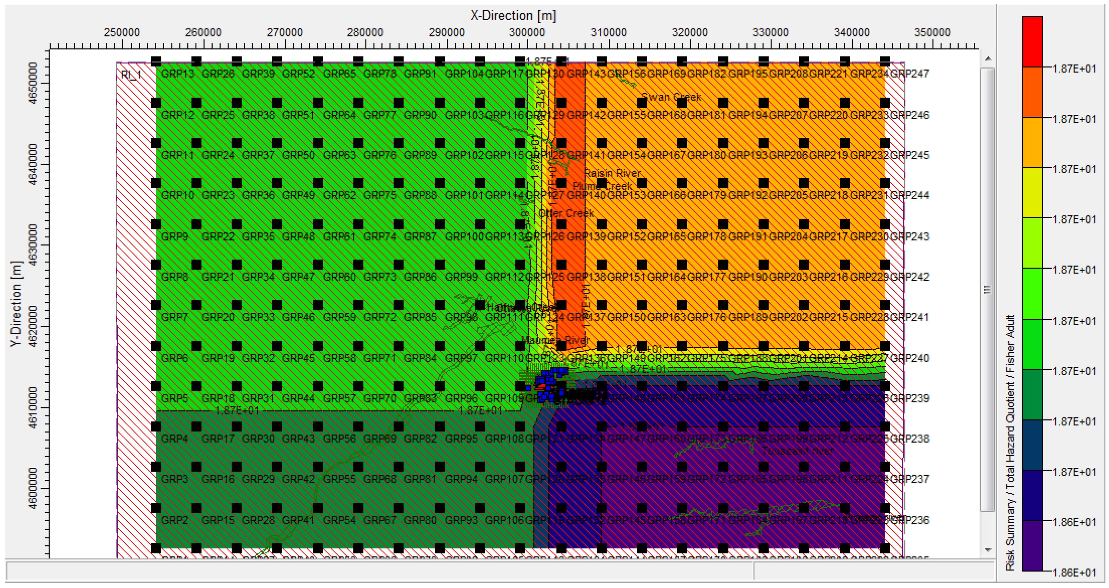
Risk Characterization

The risk characterization for the proposed plant locations was performed in accordance with HHRAP guidelines. Air dispersion modeling results were combined with toxicity information, emissions estimate and other site-specific information to generate risk and hazard values for individuals exposed to COPC emissions. The risk and hazard values for individuals could then be compared to acceptable benchmarks for human health. The magnitude and types of risks depend on the nature, duration and frequency of exposure to the selected chemicals emitted from the process and the characteristics of the exposed human receptors. Quantitative estimates of carcinogenic risks and non-carcinogenic hazards were calculated for direct inhalation exposures and indirect exposures to the COPC emissions. Estimated total carcinogenic risk was compared to an acceptable level of one case in one hundred thousand. The typical benchmark for evaluation of the estimated long-term, non-carcinogenic hazard from airborne unit emissions is 1.0. The US EPA Region 6 recommended that a hazard index (HI) benchmark of 0.25 be utilized to take background concentrations of COPCs into consideration in areas where significant industrial activity takes place. In addition, an acute hazard analysis was performed and the results were compared to an acceptable HI of 1.0. The carcinogenic risk is estimated as the probability of an individual developing cancer over a lifetime as a result of exposure to specified emissions. In this study, carcinogenic risk is estimated as an incremental probability of fatal cancer from exposure to emissions from each proposed plant for specific potential carcinogens (i.e., excess individual lifetime cancer risk).

According to the US EPA website, environmental exposures to mercury are not likely to cause cancer in humans. As a result, carcinogenic health effects will not be discussed in this analysis. The total hazard quotients estimated by the model, based on the air concentrations and depositions predicted by AERMOD for worst-case scenarios and maximum emissions from the proposed plant, were calculated. The health risk assessments for all proposed plant locations are discussed here. This risk assessment is based on the assumption that an individual living in the area surrounding the proposed locations would consume beef, milk, poultry, eggs, pork and vegetables produced from the farms in the areas surrounding these locations. The total non-cancer hazards estimated for each receptor population, for COPC, overall exposure pathways and for all proposed locations, are presented in the following sections. The US EPA generally finds non-cancer hazard indices of less than 1 acceptable. For the first proposed location, the total hazard indices are as shown in

Table 7. Total non-cancer hazards estimated for each receptor population, for COPC and overall exposure pathways for all locations of study.

Location	Resident		Farmer		Fisher
	Adult	Child	Adult	Child	Adult	Child
1	1.07E-02	3.12E-02	2.35E-02	4.86E-02	1.87E+01	1.32E+01
2	1.58E-01	4.24E-01	3.54E-01	7.32E-01	1.10E+02	7.78E+01
3	1.47E-02	3.94E-02	3.28E-02	6.78E-02	1.36E+01	9.58E+00
4	9.83E-03	2.56E-02	2.11E-02	2.79E-03	1.09E+01	7.70E+00

. It can be seen that the highest identified hazard index is for the fisher adult and fisher child exposure pathways, with predicted values of 18.7 and 13.2, respectively. These hazard indices are higher than the target hazard index of 1.

Figure 4 illustrates the contour plot of the total hazard quotient for the first location. It can be seen that the total non-cancer hazards are higher than the target hazard index of 1. In addition, it can be noted that the total non-cancer hazards vary over the area of concern. The lowest identified hazard quotient is in the south-eastern area of the proposed location. In contrast, the highest identified hazard quotient for all exposure scenarios is in the northern area (Lake Erie area) of the proposed location, with the predicted value of 18.7 at receptors 136, 137, 138, 138, 139, 140, 141, 142 and 143 for the hazard quotient. Similarly, Figure 5 shows the contour plot of the total hazard quotient for the second location. From Table 7, it can be seen that the highest identified hazard index is for the fisher adult and fisher child exposure pathways, with predicted values of 110 and 77.8, respectively. It can be seen that the total non-cancer hazards are higher than the target hazard index of 1.

It can be seen from the IRAP results that the total non-cancer hazards vary over the area of concern. The lowest identified hazard quotient is in the whole area of concern except the north-eastern area of the proposed location, with the predicted value of 109.91. In contrast, the highest identified hazard quotient for all exposure scenarios is in the north-eastern area (Lake Erie area) of the proposed location, with the predicted value of 110 at receptor 136 for the hazard quotient. For location 3, from Table 7, it can be seen that the highest identified hazard index is also for the fisher adult and fisher child exposure pathways, with predicted values of 13.6 and 9.58, respectively. It can be seen that the total non-cancer hazards are higher than the target hazard index of 1. From Figure 6, the lowest identified hazard quotient is in the whole area of concern except the northern area of the proposed location, with the predicted value of 9.58. In contrast, the highest identified hazard quotient for all exposure scenarios is in the north-western area (Lake Erie area) of the proposed location, with the predicted value of 13.6 at receptors 149, 150, 151, 152, 153, 154, 155 and 155 for the hazard quotient.

From Table 2, for location 4, it can be seen that the highest identified hazard index is also for the fisher adult and fisher child exposure pathways, with predicted values of 10.9 and 7.70, respectively. From Figure 7, the lowest identified hazard quotient is in the south-eastern area of the proposed location, with the predicted value of 7.70 at receptors 256, 243, 230, 217, 204, 191, 178 and 165. In contrast, the highest identified hazard quotient for all exposure scenarios is in the north-eastern area (Lake Erie area) of the proposed location, with the predicted value of 10.9 at receptor 141 for the hazard quotient. In conclusion, it can be seen that the fourth proposed location has the lowest total hazard quotient. These total hazard quotients are higher than the benchmarks of 1. As a result, the hazard quotients from exposure to the emissions from the fourth proposed location are expected especially for the fisher exposure pathways. Methyl-mercury is the primary form of mercury that poses health risks. Since the consumption of contaminated fish is the common pathway of human exposure to methyl-mercury, it is highly recommended that people, especially women who may become pregnant, pregnant women, nursing mothers and young children, living in the area surrounding the proposed location do not eat fish or shellfish.

For brevity of information, the contour plots for acute inhalation risk, soil, produce, beef, milk, pork, chicken and egg concentrations are not shown, but the results are discussed here. With respect to acute inhalation risk, the ambient air concentration calculated by AERMOD was compared to the non-cancer HQs for COPC to calculate the acute hazard quotient. The potential for non-cancer adverse health effects from cumulative exposure to the COPCs was estimated by summing the chemical-specific HQs. For the first proposed location, the acute inhalation quotient risk ranged from 9.08 × 10⁻⁵ to 1.51 × 10⁻⁴ for all exposure scenarios and for all sources. The acute inhalation quotient risk was less than the target hazard index of 0.25. The lowest identified hazard quotient was in the areas of Lake Erie and Toledo and in the area in between. In contrast, the highest identified hazard quotient for all exposure scenarios was found to be in the western area of the proposed location, with a predicted value of 1.51 × 10⁻⁴ for the hazard quotient. For locations 2, 3 and 4, the hazard index was found to be less than 0.25, but the highest hazard quotient was found to be in the north-western area for location 2 and south-western area for both locations 3 and 4. Among all locations, location 2 was found to have the lowest acute inhalation hazard risk. The average soil concentrations calculated from the wet and dry deposition of particulates and vapor to the soil ranged from 2.45 × 10⁻⁴ to 0.13, 1.78 × 10⁻⁴ to 2.01, 6.81 × 10⁻⁵ to 0.193 and 6.83 × 10⁻⁵ to 0.14 mg COPC/kg soil for locations 1, 2, 3 and 4, respectively. Among all locations, location 3 had the lowest soil concentration, although all soil concentrations found in these locations were within the acceptable limits. Regarding produce concentrations, the evaluation was based on the assumption that the majority of people who live in the area surrounding the proposed locations would consume fruits and vegetables grown in the vicinity of the proposed locations and may be exposed to marginally higher levels of COPCs. The produce concentrations due to direct deposition ranged from 6.54 × 10⁶ to 2.37 × 10⁻⁴, 4.43 × 10⁻⁶ to 4.373 × 10⁻³, 1.85 × 10⁻⁶ to 4.08 × 10⁻⁴ and 1.93 × 10⁻⁶ to 2.46 × 10⁻⁴ mg/kg for locations 1, 2, 3 and 4, respectively. The highest identified hazard quotient for all exposure scenarios was in the north-eastern area of the proposed location, with a predicted value of 4.08 × 10⁻⁴ mg/kg at receptor 141 for the hazard quotient. It was found that location 4 had the lowest concentration level. The results for beef, milk, chicken and egg concentrations (including soil and produce concentrations) are summarized in

Table 8. Concentrations of COPCs evaluated in locations 1, 2, 3 and 4.

COPC	Location 1	Location 2	Location 3	Location 4
Soil (mg/kg soil)	2.4481E-04 to 1.2711E-01	1.7812E-4 to 2.0133E+00	6.8108E-05 to 1.9279E-01	6.8266E-05 to 1.3595E-01
Produce (mg/kg)	6.5395E+06 to 2.3740E-04	4.4271E-06 to 4.3707E-03	1.8472E-06 to 4.0755E-04	1.9313E-06 to 2.4649E-04
Beef (mg/kg FW tissue)	8.2718E-07 to 8.1237E-04	6.0159E-07 to 1.3045E-02	2.4241E-07 to 1.2458E-03	2.6140E-07 to 8.6513E-04
Chicken and eggs (mg/kg FW tissue)	4.4613E-08 to 1.4493E-04	3.2265E-08 to 2.2937E-03	1.2337E-08 to 2.1964E-04	1.2366E-08 to 1.5488E-04
Milk (mg/kg FW tissue)	4.9078E-07 to 3.4000E-04	3.5727E-07 to 5.5037E-03	1.4470E-07 to 5.2485E-04	1.5713E-07 to 3.6137E-04
Pork (mg/kg FW tissue)	1.2554E-09 to 3.4941E-06	9.1348E-10 to 5.5324E-05	3.5269E-10 to 5.2974E-06	3.6070E-10 to 3.7333E-06

.

The emissions from all proposed locations and the potential for exposure to emissions were carefully analyzed in order to select the best location for a new industrial plant. The results indicate that the emissions from the second proposed location will have the largest potential impacts on human and other ecosystems in the area surrounding the proposed location. The emissions from the second proposed location will also pose a concern for ecosystem health, especially for the fisher adult and child scenarios. In contrast, the emissions from the proposed fourth location had the lowest potential impacts on humans and the environment in the surrounding area. Although it had the lowest potential impacts, the fisher adult and child scenarios still faced risks and hazards, in lower levels, resulting from the emissions. Based on the assumption and scenarios used to predict the potential hazards and risks associated with emissions from the proposed locations, at the proposed fourth location, the risks and hazards were found to be within or less than the acceptable range. Based on a comprehensive assessment of the potential for human health risks, it is concluded that the fourth proposed location is the best location for the new industrial plant.

5. Conclusions

The main objective of this study was to assess the potential impacts associated with the emissions of toxic air contaminants from new industrial plants in order to select the best location based on a human health risk assessment. The effects of human exposure from emissions to air from four proposed locations were considered in this study. This study was carried out in accordance with the US EPA HHRAP for hazardous waste combustion facilities. Exposure assessment was incorporated into the results of dispersion and deposition modeling with health effects known to be associated with COPC and potential exposure pathways to produce an estimated health risk. Worst-case scenarios were considered for all receptors in assuming multiple exposure conditions, where all pathways of exposure in each land use scenario were considered to be viable. The IRAP-h View model, which is based on the US EPA HHRAP, was used to calculate the transport and fate of mercury from all proposed industrial plants. The geographical area considered in this study, together with the locations of the various sources, is located in Toledo City, OH, USA. The total hazard quotient estimated by the IRAP-h View model, based on the air dispersion modeling prediction of air concentrations and depositions by the AERMOD model for the worst-case scenarios, and the maximum emissions from all proposed plants were calculated. The risk characterization was undertaken by examining the toxicity of the mercury to which individuals have been exposed and evaluating the significance of the calculated dose in the context of probabilistic risk. After a profound analysis and understanding of all results estimated by the IRAP-h View model, it was concluded that the potential exposure to emissions from the fourth proposed location (farthest east) had the lowest risk levels and represented the best location for the new industrial plant. These conclusions are based on the available pollutant exposure data for this case study and some valid assumptions used in the IRAP-h View model and AERMOD.

References

1. Visscher, A.D. Air Dispersion Modeling: Foundations and Applications; Wiley: Hoboken, NJ, USA, 2013. [Google Scholar]
2. Guldmann, J.-M.; Shefer, D. Industrial Location and Air Quality Control: A Planning Approach; John Wiley & Sons Inc.: New York, NY, USA, 1980. [Google Scholar]
3. Cai, T.; Wang, S.; Xu, Q. Monte Carlo optimization for site selection of new chemical plants. J. Environ. Manag. 2015, 163, 28–38. [Google Scholar] [CrossRef] [PubMed]
4. Seangkiatiyuth, K.; Surapipith, V.; Tantrakarnapa, K.; Lothongkum, A.W. Application of the AERMOD modeling system for environmental impact assessment of NO2 emissions from a cement complex. J. Environ. Sci. 2011, 23, 931–940. [Google Scholar] [CrossRef]
5. Zou, B.; Wilson, J.; Zhan, F.B.; Zeng, Y. Performance of AERMOD at different time scales. Simul. Model. Pract. Theory 2010, 18, 612–623. [Google Scholar] [CrossRef]
6. Macêdo, M.F.M.; Ramos, A.L.D. Vehicle atmospheric pollution evaluation using AERMOD model at avenue in a Brazilian capital city. Air Qual. Atmos. Health 2020, 13, 309–320. [Google Scholar] [CrossRef]
7. Huang, D.; Guo, H. Dispersion modeling of odour, gases, and respirable dust using AERMOD for poultry and dairy barns in the Canadian Prairies. Sci. Total Environ. 2019, 690, 620–628. [Google Scholar] [CrossRef] [PubMed]
8. Kakareka, S.V.; Salivonchyk, S.V.; Kakosh, Y.G. AERMOD application for assessment of formaldehyde emission dispersion from chipboard production. Russ. Meteorol. Hydrol. 2019, 44, 338–344. [Google Scholar] [CrossRef]
9. Amoatey, P.; Omidvarborna, H.; Affum, H.A.; Baawain, M. Performance of AERMOD and CALPUFF models on SO2 and NO2 emissions for future health risk assessment in Tema Metropolis. Hum. Ecol. Risk Assess. Int. J. 2019, 25, 772–786. [Google Scholar] [CrossRef]
10. Omidvarborna, H.; Baawain, M.; Al-Mamun, A.; Al-Muhtaseb, A. Dispersion and deposition estimation of fugitive iron particles from an iron industry on nearby communities via AERMOD. Environ. Monit. Assess 2018, 190, 655. [Google Scholar] [CrossRef] [PubMed]
11. dos Santos Cerqueira, J.; de Albuquerque, H.N.; de Assis Salviano de Sousa, F. Atmospheric pollutants: Modeling with Aermod software. Air Qual. Atmos. Health 2019, 12, 21–32. [Google Scholar] [CrossRef]
12. Matacchiera, F.; Manes, C.; Beaven, R.P.; Rees-White, T.C.; Boano, F.; Mønster, J.; Scheutz, C. AERMOD as a Gaussian dispersion model for planning tracer gas dispersion tests for landfill methane emission quantification. Waste Manag. 2019, 87, 924–936. [Google Scholar] [CrossRef] [PubMed] [Green Version]
13. Askariyeh, M.H.; Kota, S.H.; Vallamsundar, S.; Zietsman, J.; Ying, Q. AERMOD for near-road pollutant dispersion: Evaluation of model performance with different emission source representations and low wind options. Transp. Res. Part D Transp. Environ. 2017, 57, 392–402. [Google Scholar] [CrossRef]
14. Tamer, A.; Ramadan, M.A.E.; Hesham, G.; Bahnassy, M.H.; Kishk, F.M.; Selim, H.M. Heavy metals accumulation and spatial distribution in long term wastewater irrigated soils. J. Environ. Chem. Eng. 2003, 1, 925–933. [Google Scholar]
15. Afsaneh, A.; Rashid, M.; Afzali, M.; Younesi, V. Prediction of air pollutants concentrations from multiple sources using AERMOD coupled with WRF prognostic model. J. Clean. Prod. 2017, 166, 1216–1225. [Google Scholar]
16. Fernando, A.S.A.; Ricardo, C.A.; Nelson, L.C.D. Statistical evaluation of a new air dispersion model against AERMOD using the Prairie Grass data set. J. Air Waste Manag. Assoc. 2014, 64, 219–226. [Google Scholar]
17. Awkash, K.; Rashmi, S.P.; Anil Kumar, D.; Rakesh, K. Application of WRF Model for Air Quality Modelling and AERMOD—A Survey. Aerosol Air Qual. Res. 2017, 17, 1925–1937. [Google Scholar]
18. Yusef, O.K.; Pierre, S.; Adewale, M.T.; Alessandra, M.; Shirin, E.; Rajab, R. Modeling of particulate matter dispersion from a cement plant: Upwinddownwind case study. J. Environ. Chem. Eng. 2018, 6, 3104–3110. [Google Scholar]
19. Wark, K.; Warner, C.F.; Davis, W.T. Air Pollution: Its Origin and Control, 3rd ed.; Prentice Hall: Menlo Park, CA, USA, 1997. [Google Scholar]
20. USEPA. User’s Guide for the AMS/EPA Regulatory Model AERMOD; Office of Air Quality Planning and Standards Emissions, Monitoring, and Analysis Division: Durham, NC, USA, 2005.
21. Bhardwaj, K.S. Examination of Sensitivity of Land Use Parameters and Population on the Performance of the AERMOD Model for an Urban Area; University of Toledo: Toledo, OH, USA, 2005. [Google Scholar]
22. USEPA. Mercury Study Report to Congress. Available online: http://www.epa.gov/mercury/mercury-study-report-congress (accessed on 27 February 2016).
23. USEPA. Human Health Risk Assessment Protocol for Hazardous Waste Combustion Facilities; Office of Solid Waste and Emergency Response (5305W): Washington, DC, USA, 2005.
24. USEPA. Expobox. Available online: https://www.epa.gov/expobox/exposure-assessment-tools-routes-ingestion#calculations (accessed on 1 March 2021).
Figure 1. Direct and indirect exposure pathways considered in health risk assessment [23].
Pollutants 02 00030 g001
Figure 2. Receptor location identified by IRAP model.
Pollutants 02 00030 g002
Figure 3. (a) Water body and watershed polygons. (b) The layout of existing and proposed plant locations.
Pollutants 02 00030 g003
Figure 4. Contour plot of the total hazard quotient for location 1.
Pollutants 02 00030 g004
Figure 5. (a) Contour plot of the total hazard quotient for location 2. (b) Magnification of the area enclosed by white rectangle in (a).
Pollutants 02 00030 g005aPollutants 02 00030 g005b
Figure 6. Contour plot of the total hazard quotient for location 3.
Pollutants 02 00030 g006
Figure 7. (a) Contour plot of the total hazard quotient for location 4. (b) Magnification of the area enclosed by white rectangle in (a).
Pollutants 02 00030 g007