1. Introduction
The ever-increasing need for “green” energy has forced attention towards geothermal energy sources, aiming mostly at the utilization of geothermal steam to run electricity plants. Such applications require that the fluid enthalpy extracted from the reservoir is high enough to deliver enough power to the steam turbine and end up with a reasonable electric energy production rate bearing in mind that the production efficiency of such plants is very low.
The geology of Greece supports geothermal energy exploitation as various sites such as Methana and the islands of Milos, Kimolos and Nisiros lie on the so-called Aegean Sea volcanic arc. The Milos high enthalpy field has been proven to bear a reservoir temperature of 320 °C of single phase liquid water, which ends up at a slightly lower temperature at the wellhead [
1]. Well testing has shown a strong hydraulic potential with a maximum deliverable power rate of approximately 110 MW.
Clearly, the management of fields of such a size is not an easy task. Poor management may lead to the quick “death” of the reservoir by various reasons such as its inability to recharge in both hydraulic and thermal terms or, in most cases, a lack of sustainability of energy production. The reservoir lifetime may shrink to only a few decades as opposed to the commonly expected span of 100–300 years [
2]. The poor monitoring problem stems from the fact that very limited information on the state of the reservoir can be obtained at the surface. Flowrate, pressure and temperature measurements are collected at the wellhead conditions with only a few of them being measured downhole. Additionally, the number of wells is limited due to the huge cost of drilling projects, thus also limiting the number of information sampling points in the reservoir.
To anticipate that situation, we rely on combined mathematical and physics approaches to infer the state of the reservoir at each point and at each time during its life. The traditional approach requires that the reservoir simulation mathematical model is set up using all information that has been collected during the exploitation phase such as geological estimations, the interpretation of geophysical scans, well logs and production tests. Subsequently, the model is history matched to optimize its uncertain parameter values and ensure that the tuned model can reproduce the recorded production, pressure and temperature history. Finally, the tuned model is used to test various production scenarios to identify the weak points of the system and design the production scheme that optimally exploits the geothermal resource.
Two approaches can be envisaged towards reservoir modeling: distributed and lumped modeling [
3]. In the first case, the mass and heat flow differential equations are solved numerically in the reservoir domain, which in turn requires the discretization of space and time into small blocks so that the exact derivatives are approximated accurately enough by the numerical ones. Properties of interest such as pressure, temperature and gas saturation (i.e.,
,
and
, with the latter being applicable only to saturated reservoirs) can be estimated individually at any point in the reservoir, thus allowing for their detailed spatial and temporal description. The price to be paid is the need to accurately determine the rock and fluid properties at each point of the reservoir—a task that can only be accomplished approximately by means of interpolation methods. Most commercial software assumes that the rock and fluid temperature at any point in the reservoir share the same value; hence, conductivity between those two is not considered and heat is assumed to be transferred uniformly to or from them. Dirichlet-type boundary conditions—that is, fixed temperature (and/or pressure) and specific points—are considered to apply to both the rock and the fluid.
The second approach is based on the overall mass and heat balance equations that treat the reservoir as a tank, thus justifying the name of a “tank model” [
4]. Although pressure, temperature and saturation are only determined in terms of their average values over time, i.e.,
,
,
and
, such models can provide performance predictions by utilizing only average values of the rock and the fluid properties as opposed to the distributed models. Note that rock temperature
is considered independently of the fluid one, thus allowing for conduction to be taken into account individually. Of course, as mentioned above, the properties need to be history matched to reduce uncertainty and increase the model accuracy.
In this work, we consider the application of both approaches for the modeling, study and optimization of a high enthalpy field that has borrowed features of the Milos island high enthalpy reservoir in Greece. The setup of both models is considered and their ability to be history matched is examined. We focus on the overwhelming advantages of the distributed parameter modeling as well as the numerical difficulties that may be encountered that may lead to an entire lack of a physical interpretation. Such inconsistencies may completely destroy the capability of the model to provide reasonable and accurate predictions of the future behavior of the reservoir as far as both its hydraulic and thermal conditions are concerned and eventually lead to an erroneously predicted sustainability of geothermal fluid production.
2. Distributed and Lumped Parameter Models
2.1. Distributed Model Setup
The basic equations as shown below describe the conservation of fluid mass and momentum (i.e., Darcy’s law) and the conservation of heat [
5]:
that need to be solved for temperature
and hydraulic head
. The first equation states that the injection and production of fluids are responsible for the hydraulic head changes whereas Equation (2) is the vector form of Darcy’s law. Equation (3) implies that the change in the fluid and rock heat content is due to the heat transferred from and to the producing and the injecting wells, respectively, due to thermal conductivity as well as any external heat source such as magmatic intrusions.
In the formulation above, denotes the depth-integrated specific storage coefficient, is the hydraulic head, is the depth-integrated Darcy velocity, is the overall sink/source term of mass, is the overall sink/source term of internal energy, is the transmissivity tensor, is the viscosity relation function, is the aquifer thickness, is the fluid volume fraction (porosity) and is the depth-integrated conductivity tensor; and denote the fluid mass density and specific heat capacity, respectively.
Note that both the pressure and temperature are indirectly involved in the equations above through the fluid properties (sometimes those of the rock as well) [
6]. For example, the hydraulic head depends on the fluid density, which in turn depends on both
and
as well as on the phase behavior of water for conditions lying inside the phase envelope. Fluid enthalpy, compressibility and heat capacity also depend on both intensive properties whereas when a very detailed static model is available and the pressure variance is extensive, porosity compressibility might also be considered to be a function of pressure.
2.2. Lumped (Tank) Model Setup
The basic equations to describe the conservation of the fluid mass and of the fluid and rock heat are similar to those given in the previous paragraph and are listed below [
4]:
where
,
,
and
denote the reservoir rock volume, porosity, heat capacity and temperature, respectively;
and
denote the fluid density and enthalpy; and
denotes the thermal conductivity between the rock and fluid. The pressure appears implicitly in the fluid density and enthalpy as well as in the porosity when the rock is considerably elastic. The temperature appears explicitly in the equations but it also affects the fluid properties. This time rock temperature does not coincide with the fluid one and the two are related through the heat conduction term.
It can be readily seen that when comparing Equations (4)–(6) against Equations (1)–(3) all space related terms (such as gradients) have vanished and the tensors have simplified to scalars. Note that complex reservoir structures may be split into more than one tank, each one exhibiting its own temperature and pressure value that interact both hydraulically and thermally.
Subscripts
and
are used to denote the mass and heat rates taken and given to the reservoir through the producers and injectors, respectively, or through faults that contribute to the reservoir heating.
denotes the heat rate transferred to the reservoir from a magmatic intrusion and it is assumed to be given by a Cauchy-type boundary condition of the form:
where
and
denote the area and heat transfer rate between the magmatic intrusion of a constant temperature
.
Despite its simplicity, the lumped parameter model has been shown to efficiently handle the complexity of high enthalpy reservoir dynamics whilst avoiding numerical instability, as will be shown in the next section.
2.3. Supporting Algebraic Equations and State Laws
The differential equations above are further supported by physical models, closeness equations and state models [
3]. As examples, the dependence of fluid density and rock porosity on pressure and temperature might be considered. For liquid water simulations, compressed water tables or correlations can be used to determine the property values.
Note that such properties need to be quite accurate and their dependence on pressure and temperature may have a huge role in the solution. For example, as water is quite incompressible even at high temperatures, a small change in the reservoir mass content due to the mass influx and outflux (i.e., the RHS or Equation (4)) can cause a huge change in the average system pressure. Similarly, the cooling and depressurizing of a reservoir have the opposite effect on fluid density as the latter tends to increase and decrease, respectively.
2.4. History Matching
The uncertainty that is inherent to all estimated values of the reservoir parameters needs to be reduced by means of history matching [
7]. The reservoir is produced for a period of time and the well pressure and temperature are recorded together with the fluid production. Subsequently, the model is utilized to reproduce the recorded history by incorporating the flowrates observed in real life. With history matching, the model properties are regressed to minimize the difference between the recorded pressure and temperature and the corresponding values obtained by the simulator.
When high enthalpy reservoirs are considered, the pressure (rather than the hydraulic head) and temperature are measured at the wellhead and need to be converted to bottom hole values by considering the hydrostatic and frictional pressure losses as well as the thermal loss along the wells.
This step may become even more complex when considering lumped parameter models as the values utilized for their history matching need to be average ones that are not directly available. Therefore, the averaging of the recorded values needs to be done over the volume of the reservoir, which in turn requires a fair estimation of the drainage area of each well.
3. High Enthalpy Reservoir Model Setup
3.1. Static Model
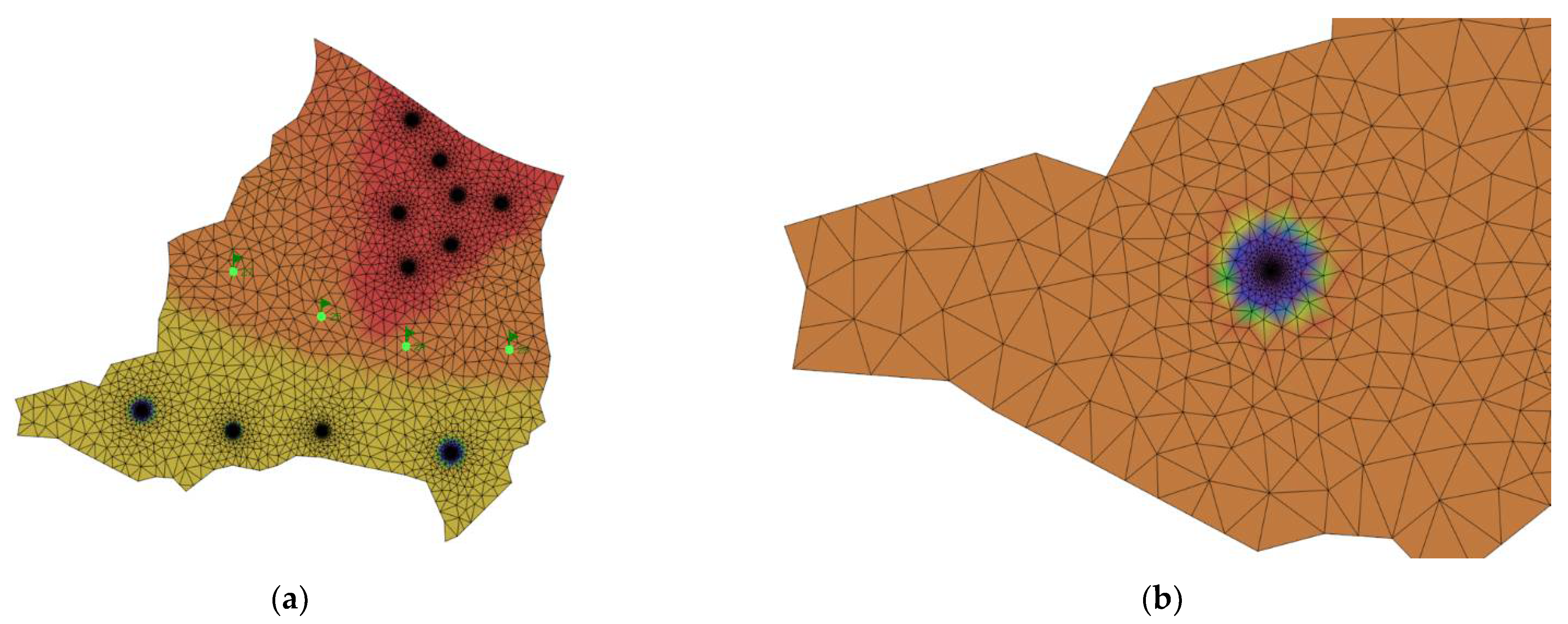
To simulate the field under study, a realistic 3D model was set up by utilizing the information available. The reservoir area was 25 km
2, its average thickness was 100 m and it was confined in that it was not affected naturally by any hydraulic source/sink term. The reservoir bottom exhibited a 15 m elevation difference in the north-south direction. The hydraulic and thermal conductivity were attributed regular values that were further interpolated based on point measurements. The wellhead pressure and temperature conditions were converted to downhole ones by considering the well effects. The reservoir is shown in
Figure 1a.
It should be noted that the geothermal field utilized in this study is a real one which lies in south Germany with its static model being developed (i.e., field dimensions, permeability and porosity distribution etc.) as suggested by the GnG group that worked on the study and analysis of that particular field. To bring it closer to the Greek high enthalpy subsurface the reservoir temperature (i.e., the effect of the magmatic intrusion) was deliberately elevated to 320 °C which is representative of the prevailing situation in Milos high enthalpy reservoir. Similarly, the depth was set equal to that of the field that was produced in the past and the pressure distribution of the original geothermal field was shifted accordingly. This procedure ensures that the static model utilized is realistic and to some extent it shares properties of the real high enthalpy reservoir in Milos.
The reservoir was heated by a magmatic intrusion that lay deeply below its bottom and forced an initial equilibration of the reservoir temperature that varied between 280 and 320 °C. The heat source continued to offer heat to the reservoir upon departing from the equilibrium. Note that the high prevailing pressure always ensured a single phase liquid phase reservoir.
To set up the distributed model, 6844 nodes were defined in four slices, thus generating 13,532 finite elements in three layers. A total of 11 wells, 7 producers and 4 injectors penetrating the reservoir were defined and the mesh was densified near the wellbore areas. The producers penetrated the top layers of the reservoir whereas the injectors were perforated along the lower ones.
To model the magmatic intrusion heat effect, all nodes in the lowest slice (bottom of the reservoir) were split into three groups and assigned appropriate
values. The north-east side of the reservoir was assigned the highest temperature (320 °C) whereas the south one was assigned a 280 °C source. The remaining part of the reservoir bottom thermal source was set at 300 °C (
Figure 1b). Note that in real life, the source temperature varies smoothly rather than exhibiting abrupt changes; however, such a setting is not possible with most available commercial geothermal reservoir simulation software.
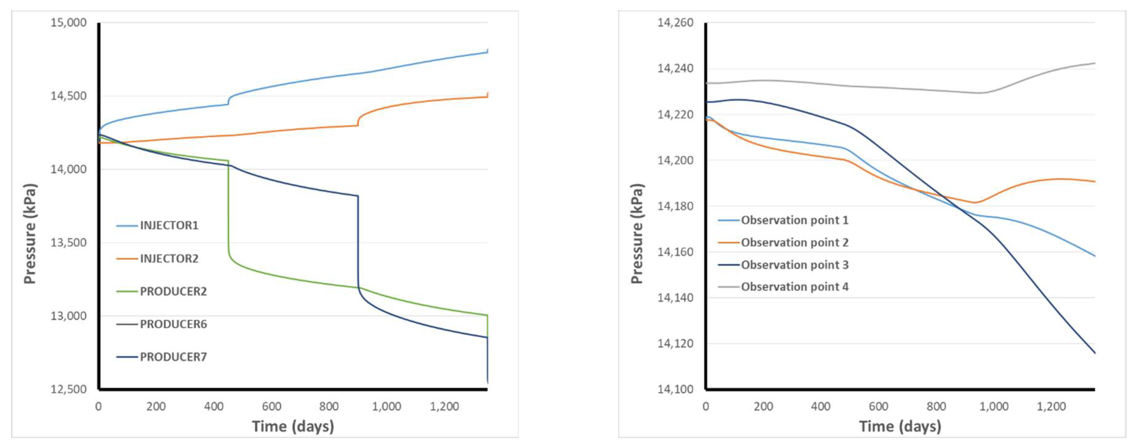
3.2. Production and Injection Schedule
As no production history data is available for the field under study, the distributed model has been considered as an already history matched one, therefore its early performance, as obtained, by solving the governing differential equations is considered to be the ground truth against which the lumped is further history matched, thus ensuring a common starting point for both approaches.
The history matching period accounted for 3.6 years (1350 days) of operation and it was separated into three different periods, as shown in
Table 1, with increasing production and injection rates. As the production of electric power was the main goal, losses in the power plant due to phase changes of up to 10% were envisaged as a result of the smaller amount of fluid injected compared with what was produced.
All three periods lasted 450 days with the second one ending on day 900 and the last one ending on day 1350. Briefly, the schedule considered the production by 3 producers (P4, P5, P6) and 2 injectors (I1, I4) for 15 months, the production of another 2 producers (P1, P2) and one injector (I2) for another 15 months and a third period of the same duration where all producers and injectors were active. This choice aimed at revealing as much as information as possible for the pressure and temperature variations with time, thus collecting useful historical data against which the material balance model was to be calibrated. On top of that, transient phenomena taking place were pronounced, thus forcing the material balance model to reproduce. This increasing production schedule was a realistic approach to what an operating company would do; starting with a small-sized plant and gradually increasing its power by drilling new wells is a common practice [
8].
The prediction scenario that followed the history matching period was set up for almost 300 years (from day 1350 to 100,000) to examine sustainability as defined in [
3] with maximum production rates, higher than those of the history matching period, of the order of 9300. The maximum heat power extracted under this scheme was equal to 162 MW before the surface and plant losses were considered.
All simulation of the distributed model were run using the FEFlow software which is capable of solving underground fluid flow problems in porous media while considering both their hydraulic and the thermal effects.


