A Response Surface Methodology Approach to Develop a Multiphysics Simulation Model of a Tensile Friction Test ^†

Abstract

High Strength Steels (HSS) are widely used in the automotive industry to reduce the vehicle’s weight and improve fuel efficiency. The press hardening process is used, for instance, to form and harden low-alloyed steel simultaneously. A deep understanding of the interfacial phenomena and the friction behavior at high temperatures is significant in describing the process, especially when considering Finite Elements (FE) analysis. In this paper, the results of a series of tensile friction tests carried out with aluminum-silicon coated low alloyed steel 22MnB5 for different values of drawing speed, temperature, and die pressure are investigated. All tests were conducted by a special test rig designed by the authors. Following the Surface Response Methodology approach, a Central Composite Design was used to identify the best fitting friction model that approximates the friction coefficient behavior depending on the main testing parameters. The identified model can explain up to 88% of the variability of the response variable and predict the friction coefficient with acceptable error. In conclusion, a FE multi-physical model of the tensile friction test, which combines a structural and a thermal analysis, was created and validated by LS Dyna software simulations.

1. Introduction

In the last decades, High Strength Steels (HSS) have been introduced in the automotive industry to reduce the weight of vehicles, improve safety, and reduce CO₂ emissions. However, the formability and shape accuracy of HSS decrease with increasing strength. An approach to reduce the springback behavior at cold forming and to improve the formability is press hardening, which allows adjusting the desired properties of the final product in terms of the microstructure, surface condition, and strength. However, to optimize this process, knowledge of the interfacial phenomena and material behavior at high temperatures is required.

Nowadays, there is a great demand for effective process design using Finite Elements (FE) analysis to predict the feasibility of forming complex shaped parts. In particular, when the press hardening process is analyzed, the numerical results are strongly affected by the state of the contact between the blank and the tool. Therefore, the friction coefficient plays an important role in numerical simulation. Several studies have been conducted to understand how the friction coefficient varies during the forming phase of the process.

Yanagida [1] carried out experiments on 22MnB5 steel, which showed that the mean coefficient of friction decreases with increasing temperature up to 300 °C while above 300 °C it tends to increase with rising temperatures. Moreover, the coefficient of friction increases with accelerated drawing speed up until the value of 10 mm/s is reached. Above this value, the coefficient of friction becomes constant. The mean coefficient of friction is independent of the die pressure in the range of compression load from 15 MPa to 45 MPa.

Ghiotti [2] presented an investigation to identify the friction coefficient between the 22MnB5 blanks and the dies as a function of the most relevant process parameters: normal pressure, blank temperature, sliding velocity, and tool surface finishing. The results from high-temperature pin-on-disk experiments show that the friction coefficient is not affected by both the sliding speed or surface quality of the pin. On the contrary, it was found that the blank temperature and contact pressure are the process parameters with a major influence on the friction coefficients.

Mozgovoy [3] studied the influence of pressure, sliding velocity, tool temperature, and sheet coating on the friction behavior of tool steel specimens sliding against 22MnB5 steel sheets under press hardening contact conditions. It was discovered that the influence of sliding velocity on the coefficient of friction is negligible, while there is a decrease in friction coefficient with increasing load. A higher load leads to a lower and more stable coefficient of friction independent of the applied sliding velocity or material.

The aim of this research is to identify and validate a friction model capable of predicting the value of the coefficient of friction during the tensile friction test of high-strength steel 22MnB5. The relevant varying test parameters are contact pressure, speed, and temperature of the steel strip. In addition, a statistical analysis based on the Response Surface Methodology (RSM) is conducted to identify a regression equation that could approximate the friction coefficient behavior and understand which process parameters influence the coefficient of friction.

Considering the high costs of test series, a multi-physical model of the friction tensile test that combines a structural and a thermal analysis, was created by the FEA software LS Dyna. It can predict the behavior of the steel strip during the test.

2. Materials and Methods

A scheme of the flat drawing testing apparatus used to measure the coefficient of friction at high temperatures is shown in Figure 1.

By the tensile friction test, the friction coefficient can be evaluated using Equation (1):

$$\mathsf{\mu }=\frac{F_T}{2·F_P}$$

(1)

where F_T is the tensile force applied to the specimen; F_P is the compressive force between the jaws. The testing device used to apply the pressure on the die and the tensile load on the steel strip is the Instron Structure Testing System Portal 100 kN. This testing machine is equipped to apply vertical compression and horizontal tension forces. Both are driven by pneumatic pistons, capable of applying a maximum force of 100 kN. Before passing through the die, the strip was heated by a custom-shaped inductor powered by an Eldec HFG 50 generator, which has a maximum output of 50 kW. An Optris Quotient pyrometer is used to evaluate the temperature value reached by the samples in the heating phase. The specimens were pulled through a pair of jaws applied to an area where the specimen faced the test pressure. This experimental setup was created in the laboratories of the Fraunhofer IWU (Dresden, Germany) with equipment provided by the Chemnitz University of Technology (Chemnitz, Germany).

The examined material, 22MnB5 steel, is extensively used for the press hardening process because of its excellent formability at elevated temperatures and high strength after hardening. To prevent oxidation of the metal sheet while press hardening, coatings are used. Currently, the most common is an aluminum-silicon-based layer. The specimens used have a width of 30 mm, a length of 1250 mm, and a thickness of 1.5 mm. The samples have an Al-Si coating that has been diffused on the base material by specific heat treatment. The material used for the jaws is 1.2367 tool steel; it is widely used to produce press-hardening tools because of its high hardness and wear resistance.

To identify a friction model based on the experimental data produced, the Response Surface Methodology (RSM) was used. As reported by Erto [4], it is a technique that analyses the relationships between several independent variables or factors, known as predictor variables, and one or more dependent variables, known as response variables. The main objective of RSM is to use a sequence of designed experiments to obtain an optimal response.

The Central Composite Design (CCD) is the most commonly used response surface-designed experiment. The CCD consists of three distinct sets of experimental runs:

• A factorial (or fractional factorial) design in the factors studied; each has two levels;
• A set of center points, experimental runs whose values of each factor are the medians of the values used in the factorial portion. This point is often replicated to improve the precision of the experiment;
• A set of axial points, experimental runs equal to the center points except for one factor, which will assume values below and above the median of the two factorial levels. These allow us to estimate curvature.

Studying k factors using Central Composite Design requires a number of design point (N) evaluations equal to:

N = 2^k + 2k + n

(2)

being n the number of repetitions in the center point.

The analyzing aspect of this design can be explained by the following equation:

$$\begin{array}{c}Y=b_0+b_1{X}_1+\cdots +b_k{X}_k+b_{12}{X}_1{X}_2+b_{13}{X}_1{X}_3+\cdots +b_{k-1,k}{X}_{k-1}{X}_k+\\ b_{11}{X}_1^2+\cdots +b{k}_k{X}_k^2+ϵ\end{array}$$

(3)

The above equation represents the quadratic model, which is near to the optimization. In this equation: Y = Dependent variables, X₁, …, X_k = independent variables, b₀ = overall mean response, b₁, …, b_k = regression model coefficients, K = number of independent variables, ϵ = error. Equation (3) is a mathematical model to approximate the observed values of the dependent variables y, that considers the main effects for factor (X₁, …, X_k), their interactions (X₁X₂, X₁X₃, …, X_k−1X_k) and their quadratic components (X₁², ……, X_k²).

To determine the local axial point, it is necessary to identify the alpha value in the CCD model. It can be calculated in the following way by Equation (4):

$$\alpha ={[\frac{2^{k-f}{n}_c}{n_s}]}^{\frac{1}{4}}$$

(4)

With: k = number of factors; f = fraction of the design; n_c = number of corner points; n_s = number of star points. The main factors that influence the press hardening process, according to the literature, are:

• Metal sheet temperature at which the semi-finished product enters the tool before being formed;
• Sliding speed, namely the relative speed between the die and the metal sheet during the forming phase of the piece;
• Mold pressure; that is, the pressure value with which the metal sheet is formed.

These three parameters have been chosen as control factors of the design of the experiments study. Regarding the response variable, the friction coefficient has been selected. The typical ranges of values obtained by these parameters in the press hardening process are the following:

• Metal sheet temperature: 400–720 °C;
• Sliding speed: 10–80 mm/s;
• Pressure: 10–40 MPa.

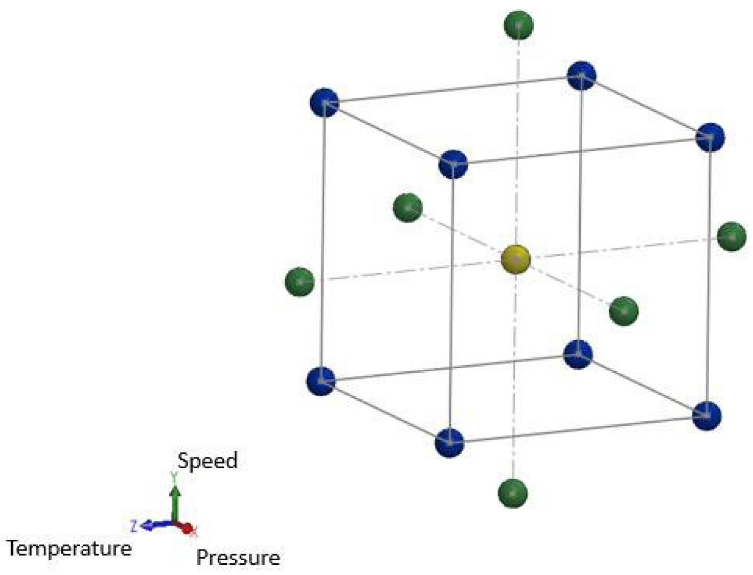
The values above were identified from the literature. A 3-factor CCD was created from these values, with 2 levels for each factor. In Figure 2, the blue dots represent the base factorial design, with 3 factors and 2-levels for each factor, the yellow dot represents the center point, and the green dots represent the axial points.

The control factors (Temperature, Speed, and Pressure) have been set at two levels each that are listed in

Table 1. Control Factors levels.

	Level −	Level +
Temperature [°C]	465	655
Speed [mm/s]	24	66
Pressure [MPa]	16	34

. Therefore, the base factorial design consists of 2³ = 8 combinations of parameters.

A number of repetitions equal to 6 were chosen for the central point. Using Equation (4), the number of tests to be performed is 20. To conduct this analysis, the statistical software Minitab has been applied.

This design of experiments was created using the study of Lanzotti [5] as a reference.

FEA Model

As the tensile friction test involves large displacements and thermal exchange, an explicit approach has been used to model and simulate the process. Furthermore, a multiphysics model must be created that combines a structural and thermal analysis. The creation of the models started with the integration of the applied geometries. As the process presents symmetry, it was possible to study one-half of the complete geometry. For the mesh of the parts, solid type elements were used with a mean size equal to 0.5 mm for the strip and 2 mm for the jaws. Regarding the material properties, for the jaws, the rigid Material (*MAT_RIGID) is used. The material used for the strip is CWM (*MAT_CWM). This is a thermo-elastic-plastic material model with kinematic hardening dependent on temperature. The component’s thermal properties have been modeled using a thermal isotropic material (*MAT_THERMAL_ISOTROPIC) for the jaws and *MAT_THERMAL_CWM for the strip.

To reproduce the same loading conditions of the tensile friction test, all the degrees of freedom of the jaws were constrained except for the vertical displacement of the upper jaw. Pressure at interfaces between the strip and jaws was generated by applying a vertical load along the top face of the upper jaw. To move the strip at a given speed, a displacement history was imposed on the nodes of the end face of the strip. Finally, an initial temperature value of 550 °C is applied to the strip, which during the tensile friction test is heated by an inductor to a predetermined temperature value. To model the contact between the model components, the *CONTACT_AUTOMATIC_SURFACE _TO_SURFACE subroutine was chosen. Moreover, it was chosen to adopt the same value for the static and dynamic friction coefficient since we are interested in the traction force trend when we are in the dynamic regime of the test.

3. Results

All the tests were carried out by using the test parameters’ combinations given by the Central Composite Design, and the corresponding results have been analyzed by the statistical software Minitab. According to Equation (5), the following regression equation describes the friction coefficient as a function of the control factors (temperature, speed, and pressure), with X₁ the strip speed, X₂ the strip temperature, and X₃ the jaws pressure:

$$\begin{array}{c}\mu =1.252-0.00549·X_1-0.002063·X_2-0.0191·X_3+0.00032·\\ x_1^2+0.000002·x_2^2+0.000456·x_3^2+0.00005·X_1{X}_2-0.000106·\\ X_1{X}_3-0.000003·X_2{X}_3\end{array}$$

(5)

To verify if this regression model gives reliable predictions, the coefficient of determination, $R^2$, is studied. One problem with the R-square parameter is that it increases each time an independent variable is added to the model, even though this variable is not explanatory at all. To avoid this situation, in regression models with many independent variables, it is preferred to analyze the value of the adjusted R-square ($R_{adj}^2$) and predicted R- square ($R_{pred}^2$). For ourmodel, the values of $R^2$, $R_{adj}^2$ and $R_{pred}^2$ are shown in

Table 2. Model summary of the first model.

S	R-sq (${\mathit{R}}^2$)	Adjusted R-sq (${\mathit{R}}_{\mathit{a}\mathit{d}\mathit{j}}^2$)	Predicted R-sq (${\mathit{R}}_{\mathit{p}\mathit{r}\mathit{e}\mathit{d}}^2$)
0.0212	95%	90%	79%

.

The values of $R^2$ and $R_{adj}^2$, which are equal respectively to 95% and 90%, indicate a model having independent variables that succeed in explaining almost entirely the variability of the response variable around its average. In other words, knowing the values of the independent variables, it is possible to predict with acceptable accuracy the value of the response variable. The value of predicted R-square, equal to 79%, indicates that the model manages to predict the response variable well. Another kind of analysis allowing for checking the model accuracy is the analysis of variance (ANOVA), also carried out by the Minitab code.

Of all the considered factors, only those with a p-value lower than our confidence level, which has been taken equal to 0.05, are statistically significant. It can be seen in

Table 3. ANOVA for the first model.

Model Components	p-Value
Speed	0.000
Temperature	0.000
Pressure	0.001
Speed × Speed	0.088
Temperature × Temperature	0.011
Pressure × Pressure	0.000
Speed × Temperature	0.225
Speed × Pressure	0.027
Temperature × Pressure	0.722

that all 3 main parameters (temperature, velocity, and pressure) affect the friction coefficient. It is also evident that some terms are not significant to the model, namely speed × speed, speed × temperature, and temperature × pressure.

To see how the $R^2$ values vary, a new model was created that does not account for the non-significant terms identified above. In this case, the new regression equation may be written as:

$$\begin{array}{c}\mu =1.135+0.00042·X_1-0.002015·X_2-0.02139·X_3+0.000002·X_2^2\\ +0.000456·X_3^2+0.000106·X_1{X}_3\end{array}$$

(6)

The corresponding values of $R^2$, $R_{adj}^2$ and $R_{pred}^2$ are given in

Table 4. Model summary of the second model.

S	${\mathit{R}}^2$	${\mathit{R}}_{\mathit{a}\mathit{d}\mathit{j}}^2$	${\mathit{R}}_{\mathit{p}\mathit{r}\mathit{e}\mathit{d}}^2$
0.0233	92%	88%	79%

.

As expected, both $R^2$ and $R_{adj}^2$ decrease slightly while $R_{pred}^2$ remains un-changed. The decrease of $R^2$ and $R_{adj}^2$ is due to the smaller number of factors that constitute the model. However, since this decrease is small, we may say that the eliminated factors contribute little to the explanation of the model. In addition, the unchanged value of predicted $R^2$ indicates that removing those factors does not affect the model’s ability to predict COF values. 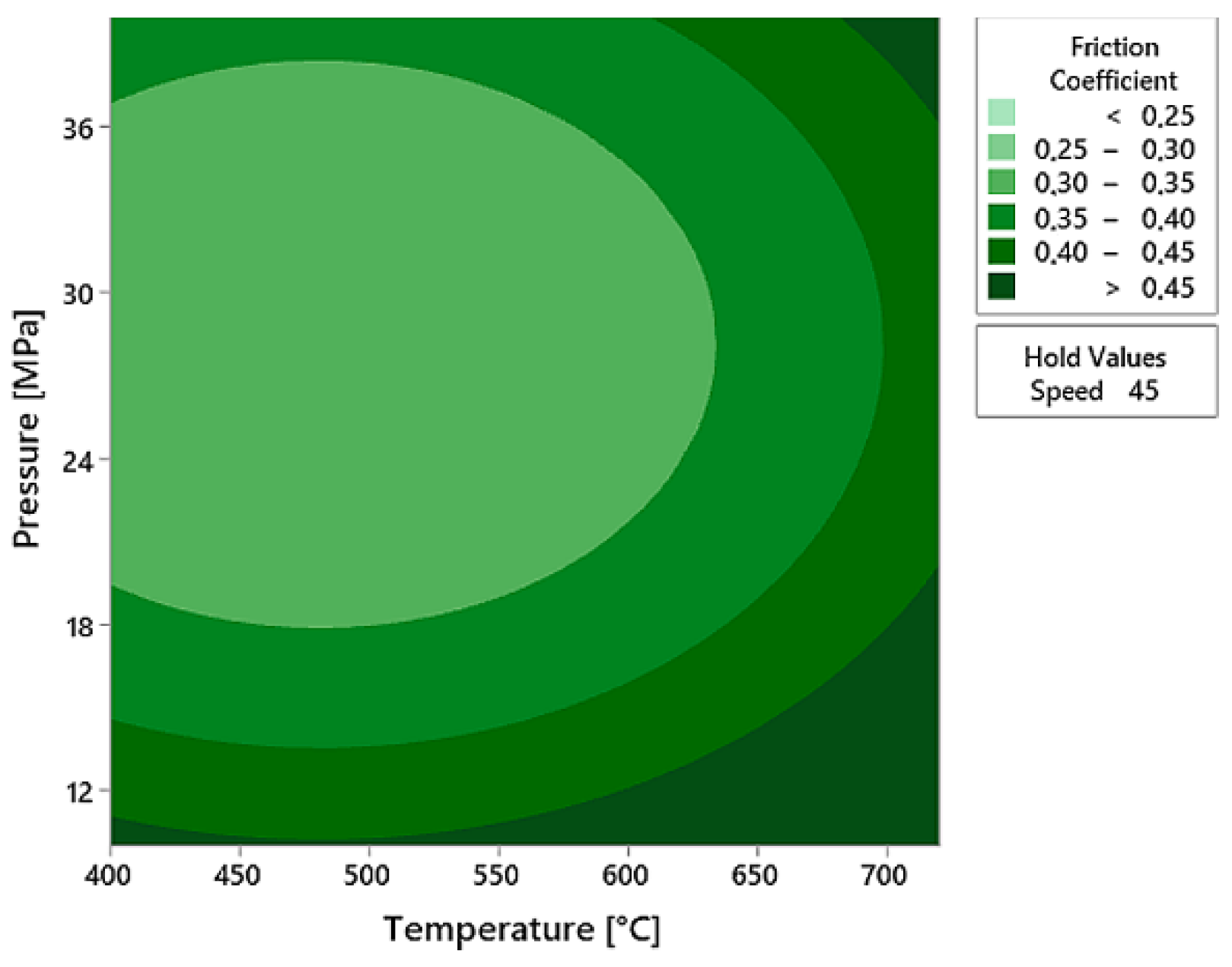In Figure 3 and Figure 4, the contour plots of the model adopting only the significant factors are reported. They highlight the trend followed by the friction coefficient as the combinations of control parameters vary.

Figure 3a shows how, for a fixed pressure value (25 MPa), the friction coefficient increases as temperature increases and speed decreases; this trend is similar to that obtained by Yanagida [1]. In Figure 3b, for a fixed temperature value of 560 °C, the COF increases as speed decreases and assumes an unusual behavior as pressure varies. In Figure 4, for a value of velocity equal to 45 mm/s, the COF decreases when the temperature varies between 400 °C and 500 °C and increases to over 500 °C. This trend can be explained by the fact that for high-temperature values, adhesion phenomena occur between the jaws and the strip, leading to an increase in tensile force and, consequently, in the COF. Instead, regarding the pressure effects, the trend is uncertain, and further studies are required to understand better the correlation between this parameter and the response variable. The observed trends are new compared with those that emerged from the state-of-the-art analysis.

FEA Results

The numerical results are reported for one arbitrarily chosen combination of parameters. In particular, the combination of parameters chosen is the following:

• Metal sheet temperature: 550 °C;
• Sliding speed: 45 mm/s;
• Mould pressure: 25 MPa.

The main aim of the FE simulation was the analysis of the stress field acting in the strip during the friction test. In Figure 5, a plot of the strip Von Mises stress field is shown. It corresponds to the last steps of the analysis when all mechanical and thermal transient effects have been overcome, and both stress and thermal field in the strip region close to the jaws are stationary.

In Figure 5, the upper jaw is not shown to allow better visualization of the stress field. It can be seen in this figure the area of the strip that is most stressed is at the exit of the jaws. In particular, in this region, Von Mises stress attains the maximum value of 181 MPa at the edges of the strip. The part of the strip pressed by the jaws has lower stress and, in some areas (the ones in blue), is almost free of stress. During the test, the strip does not deform because the stress generated is lower than the yield stress of the material at 500 °C. Another parameter of interest is the tensile load (the force along the x-axis) that is applied at the end of the specimen to pull it through the jaws. It assumes a constant trend during the performance of the test. For this simulation, the average tensile force applied to the strip is about 7.23 kN. Finally, regarding the heat transfer between the components, the strip temperature decreases from the value of 550 °C attained in the inductor heater to the value of 470 °C reached at exiting the jaws. Consequently, we may affirm that the average thermal gradient in the process zone was equal to:

ΔT_strip = 550 °C − 470 °C = 80 °C

(7)

The values of the average tensile force and thermal exchange obtained in the simulation are consistent with the ones obtained in the experimental tests.

4. Discussion

Of the two friction models that have been built, the one that considers only significant factors has to be preferred since it has a simpler and equally reliable regression equation to predict the COF. To test this model, a series of random combinations of parameters were chosen. From there, the friction coefficient was calculated using the identified regression equation, and the estimated COF value was compared with the experimental COF evaluated with a tensile friction test.

It is well known that when a statistical estimation of a parameter is carried out to quantify the estimated accuracy, a range of the probable values, called confidence interval (CI), for that parameter is identified. For this study, a confidence level of 95% has been chosen, and starting from the punctual estimates carried out by the model, the extremes of the CIs were calculated by adding and subtracting the standard deviation.

For the parameter combinations used as testers, the estimated COF value was calculated using the regression model given by Equation 6. With these results, a graph was created where on the abscissa axis, the identifying number of the parameters combination is reported while the ordinates are referred to as the Mean COF. In addition, for each parameter’s combination, the estimated COF value (orange indicator) with the corresponding confidence interval and the COF value evaluated by experimental data (blue indicator) are reported.

As proven in Figure 6, for parameter combinations 4, 5, 6, 8, 9, 11, and 13, the experimental COF lies inside the CI. On the other hand, for combinations 1, 2, 3, 7, 10, and 12, the experimentally evaluated COF value is outside the CI. A deeper analysis of these parameter combinations reveals that, except for combination 3, all combinations are at the upper extremes of the chosen parameter ranges. Hence, we deduce that the model is not fully reliable for extreme values of the selected control parameters, and more measurements are required to refine the model. In addition, by inspection of Figure 6, it is noted that the error does not have a uniform distribution over the response surface. In particular, the error is smaller at the center of the response surfaces and increases moving toward the response surface boundary. This limits the applicability of the identified friction model.

5. Conclusions

Starting from the experimental tests carried out for different parameter combinations, a friction model was identified. Initially, an analysis of variance was conducted, and, with the help of a Pareto chart, no significant factors of the starting model were found. Then a reduced model, which considered only the significant factors, was identified. It is capable of explaining a large part of the variability of the response variable, which shows a value of $R^2$ and $R_{adj}^2$ equal to 92% and 88%, and it is also good to predict the friction coefficient for new observation, with a value of $R_{pred}^2$ equal to 79%.

A multiphysics model was created in the LS-Dyna FE simulation environment to reproduce the tensile friction tests conducted experimentally. The model couples a structural analysis to evaluate the magnitude of the forces for a certain combination of parameters and a coefficient of friction, and a thermal analysis to quantify the heat transfer that occurs between the various components.

So far, a design of experiments that provides only one repetition for each parameter combination has been chosen. Better results could be reached if more repetitions were taken for the parameter combinations used to create the model. Hence further studies have to be planned to better clarify the relationship between the friction coefficient and applied pressure.