Mastering the Complexity of Incremental Forming: Geometry-Based Accuracy Prediction Using Machine Learning ^†

Abstract

The envisaged flexibility of Single Point Incremental Forming is contradicted by its highly complex deformation behavior, making the process easy to implement but difficult to fully control. This paper describes a regression method that uses Gradient Tree Boosting to predict the deviations for a given input geometry, which can replace the physical part production needed for the optimization of generating toolpaths. This paper elaborates on the calculation of the geometric features used by the regressor and the selection of an appropriate training dataset. The method is validated using a generated dataset of fully freeform ellipsoid workpiece geometries.

1. Introduction

Despite years of supporting research, commercial use of the Single Point Incremental Forming (SPIF) process remains limited. The main reason for this, is the inadequate accuracy of the produced parts due to the elastic springback and unwanted plastic deformations occurring in-process. Different strategies have been proposed to combat the resulting inaccuracy: removing its source through modification of the process itself, optimizing the process parameters or compensating the generating toolpaths [1,2]. Since the occurrence of unwanted deformations is inherently linked to the SPIF process, the last method seems the most efficient to improve accuracy without increasing process complexity. The main problem is that in a conventional approach multiple iterations are typically needed in order to obtain a toolpath that provides a satisfactory result. This implies multiple resource consuming production runs or time-consuming full simulations.

Machine learning is introduced here as a tool that enables the conversion of generic process knowledge to a predictive model that provides new opportunities for softwarebased control. The method proposed in this paper has been validated with clusters of similarly shaped workpiece geometries and will be illustrated for a set of ellipsoid fully freeform part shapes.

The accuracy of a produced workpiece can be resolved by locally calculating the deviations to the desired CAD (Computer Aided Design) model. Often, the workpiece consists of a desired component embedded in a larger sheet to facilitate production. In this case, it may be desirable to only compare the CAD data of the part rather than the full workpiece. Taking these contexts into account, the alignment of the actual measured and nominal CAD surfaces has a big influence on the calculated accuracy. The deviation of a vertex belonging to the actual surface can also be defined in a number of different ways [3]. When aiming to compensate for process inaccuracies, it is advisable to align the measured surfaces to the production frame of reference. In this way, the calculated deviations clearly show over- or under-forming behavior that needs to be counteracted in order to produce an accurate workpiece.

By calculating the deviations normal to the actual surface, these can be represented as a one-dimensional magnitude vector, which constitutes a pragmatic solution for the generation of compensated workpiece geometries on one hand and opens opportunities for the use of Machine Learning techniques for the prediction of these deviation values.

2. Predicting Workpiece Accuracy

Research by Verbert et al. [4] and Behera et al. [5] has demonstrated a strong link between part geometry features and the resulting workpiece accuracy. The inherent geometric stiffness of the SPIF part, depending on local wall angles and curvatures, plays an important role in the deformation behavior of the workpiece. Using a spline-based regression approach, it was feasible to create an offline prediction model that could be used to compensate specific part features (cones, pyramid walls, etc.). The translation of this type of approach to complex freeform geometries was achieved using the power of machine learning methods to process a large dataset of highly variable geometric parameters. The proposed methodology leverages this prior knowledge by selecting parameters that influence part accuracy.

2.1. Describing Freeform Geometry

In order to preserve the workflow of the non-automated iterative compensation, a vertex-based approach is used. For each vertex belonging to the input mesh, geometric parameters are calculated describing the local geometry. These parameters are subsequently used by the regression method to generate predictions for the deviation magnitude. The vertex-based parameters are selected to be compatible with complex asymmetric freeform parts and can be classified in one of following categories: position indicators, process limit indicators, curvature-based parameters, and geometric features, as listed in

Table 1. Vertex-based geometric parameters.

Category	Parameter	Calculation Details
Curvature	Parallel Curvature	Locally parallel to backing plate plane
	Normal Curvature	Locally normal to backing plate plane
Position	XY-Backing distance	Closest XY-distance to backing plate
	XY-Top distance	Closest XY-distance to deepest point
	Z height relative	(0, 1), within workpiece
	Z height absolute	Height in mm, for comparison between different workpieces
	Roll direction factor	Angle between local toolpath direction and sheet rolling direction
Process limits	Wall angle	Local angle defined by vertex normals
	Wall thickness factor	Residual thickness fraction using sine rule
Geometric features	Planar factor	Small principal curvatures
	Saddle factor	Large negative first principal curvature and large positive second principal curvature
	Parabolic Convex factor	Large positive first principal curvature and small second principal curvature
	Convex factor	Large positive principal curvatures
	Parabolic Concave factor	Large negative first principal curvature and small second principal curvature
	Concave factor	Large negative principal curvatures

. The use of the STL (Surface Tessellation Language) format to describe workpiece geometry means curvatures must be estimated using the orientation of the surface facets. The vertex normals can be estimated using the neighboring facets [6]. These vertex normals are then used to analytically calculate the curvature tensors for the individual facets following the approach reported by Theisel et al. [7]. From the curvature tensor, the principal curvatures κ₁ and κ₂ can be calculated, where κ₁ is the maximum and κ₂ the minimum local curvature, occurring in orthogonal directions (κ₁ ≥ κ₂). These principal curvatures are further converted to curvatures in directions parallel and normal to the backing plate.

The feature recognition methods developed by Verbert [5] and Behera [6] are not readily transferrable to freeform surfaces. A curvature-based approach however does lend itself to the classification of general freeform topology types or features. Based on the sign and magnitude of the principal curvatures κ₁ and κ₂, six different freeform features can be categorized: planar, saddle, convex, parabolic convex, concave, and parabolic concave. Convex and parabolic convex features with a high curvature tend to provide geometric stiffness resulting in more accurate parts, while planar features are most susceptible to springback and unwanted plastic deformation.

It is possible to link a single unique feature to each vertex based on its local curvatures, but when dealing with complex freeform shapes, this results in a semi-arbitrary definition of discrete feature borders. A more natural approach is the use of a fuzzy feature classification. Here, each vertex can get assigned a score for each of the feature categories. The classification is based on the calculation of two measures to determine the ‘flatness’ and ‘curvedness’ of a principal curvature. The formulas are shown in Equations (1) and (2):

flatness = {|κ| ≤ L: 1/(1 + |κ|) − 1/(1 + L) × |κ|/L, 0},

(1)

curvedness = |κ|/H × [1 − (H − |κ|)/H],

(2)

Here κ can be substituted by either κ₁ or κ₂. A threshold L is selected where curvatures can be considered ‘low’ for categorization, this threshold determines the cutoff point of the flatness measure. Since curvature values can get arbitrarily large, an upper limit H is used to control the curvedness factor: At a curvature of H, the curvedness measure will be equal to 1. Both flatness and curvedness functions are shown in Figure 1 for L = 0.01 (corresponding to a curvature radius of 100 mm) and H = 0.02 (corresponding to a curvature radius of 50 mm). The resulting overlap between both measures allows for the fuzzy classification of the principal curvature values. The full feature classification and score calculation is summarized in

Table 2. Calculation of curvature based geometric parameters.

Geometric Feature Score			Curvature Condition		Score Calculation
Planar factor			-		flatness(κ1) × flatness(κ2)
Saddle factor			κ1 × κ2 ≤ 0		curvedness(κ1) × curvedness(κ2)
Parabolic Convex factor			κ1 ≥ 0		curvedness(κ1) × flatness(κ2)
Convex factor			κ1, κ2 ≥ 0		curvedness(κ1) × curvedness(κ2)
Parabolic Concave factor			κ2≤ 0		flatness(κ1) × curvedness(κ2)
Concave factor			κ1, κ2≤ 0		curvedness(κ1) × curvedness(κ2)
	Examples		(L = 0.01, H = 0.02)
κ1	κ2	Plan.	Sad.	Par. Conv.	Conv.	Par. Conc.	Conc.
		0	-	0	6.250	-	-
0.050	0.020	(0%)	(0%)	(0%)	(100%)	(0%)	(0%)
		0	-	0.500	0.063	-	-
0.020	0.005	(0%)	(0%)	(89%)	(11%)	(0%)	(0%)
		0	0.015	5.625	-	0	-
0.020	−0.001	(0%)	(<1%)	(>99%)	(0%)	(0%)	(0%)
		0.400	<0.001	0.050	-	0.005	-
0.005	−0.002	(>87%)	(<1%)	(11%)	(0%)	(1%)	(0%)
		0.400	-	-	-	0.050	<0.001
−0.002	−0.005	(>88%)	(0%)	(0%)	(0%)	(11%)	(<1%)
		0	-	-	-	0.500	0.063
−0.005	−0.020	(0%)	(0%)	(0%)	(0%)	(89%)	(11%)
		0	-	-	-	0	6.25
−0.020	−0.050	(0%)	(0%)	(0%)	(0%)	(0%)	(100%)

. For all features except planar, an extra condition is imposed that looks at the sign of either one or both principal curvatures. This way, categorization as convex, concave or saddle remains mutually exclusive. The accumulated score vector is normalized, making the sum of scores equal to 1 for every vertex. Depending on the local geometry, a vertex can still be classified as a single feature if its score is 1 for one feature and 0 for the others, some possible combinations are demonstrated in the latter half of Table. In transition zones between geometric features, the feature scores will be much more distributed. This has two advantages: firstly, it indicates how close a vertex is located to the theoretical edge of a geometric feature, and secondly, the scores indicate which other features are expected to be found in its direct neighborhood. This is valuable information for the prediction algorithm, since feature interaction was shown to be an important factor correlated to the workpiece deviations [5].

2.2. Gradient Tree Boosting Regression

In total, a 15-dimensional parameter vector, calculated for each vertex data point, is used to predict the normal deviations. Since an average workpiece STL input easily contains thousands of vertices, the chosen regression method should be able to handle relatively large (O(106)) multidimensional datasets. When observing the complex relationship between deviations and individual parameters, it becomes clear that the required machine learning method needs to express highly nonlinear behavior.

Boosting is a so-called ensemble method that combines the predictions of a large number of simpler base regressors instead of using a single complex model, such as Neural Networks. The advantage of boosting methods is that they offer good generalizability and scalability [8].

A well-documented implementation of the boosting regressor is Gradient Tree Boosting (GTB) [9], which uses simple decision trees as base regressors due to their interpretability and robustness. By choosing an appropriate maximum depth of the tree regressors, the tree can represent highly complex if this then that behavior, making it compatible with the feature-based prediction methodology. In the construction of the boosting regressor, new base learners are added over several iterations, fitted to the residual prediction obtained by the combination of the preceding regressors. With appropriately chosen input parameters, the regressor will perform gradient descent to monotonously decrease the regression error, terminating the addition of new regressors when the accuracy improvement becomes too small.

Each decision tree regressor is constructed by repeatedly calculating split points that separate the data into two subsets, creating branches. The best split point is the parameter value that minimizes the error of the subset residuals. For this work, a Least Squared Error (LSE) approach is selected to capitalize on the full spectrum of the sparsely and non-uniformly distributed parameter combinations. Evaluating the tree regressor for a new data point is as simple as determining which leaf in the tree the data point belongs, based on its parameter values (Table 1). The prediction for the point is then the mean training residual attached to that leaf.

2.3. Reconstructing a Spif Output Geometry

The predicted deviations can be used to reconstruct a predicted SPIF output mesh. This is performed by individually offsetting each vertex of the input mesh in its local normal direction using the predicted deviation values. Because the prediction is based on the calculated vertex values, which are still influenced by the triangulation of the mesh, the resulting output surface can be noisy. It is advised to use a local smoothing technique to remove these random numerical errors. In order to maximally preserve the predicted geometry, Taubin smoothing, which uses a filtering approach is used here. This way, high frequency oscillations, which physically cannot occur in produced sheet metal parts, can be effectively removed, improving the quality of the prediction.

3. Accuracy Prediction Validation for Ellipsoid Geometries

3.1. Geometries and Materials

3.1.1. Training Data

The different workpiece shapes were defined by generating ellipsoids using six workpiece parameters (large and small diameter, z height, x and y offset of the center point and angle offset), see

Table 3. Ellipsoid training and test set workpiece parameters.

	d [mm]	D [mm]	h [mm]	x [mm]	y [mm]	α [°]
Min	30	30	30	0	0	0
Max	75	75	40	15	15	45
Training geometries
Sphere 30 1	30	30	30	15	15	45
Ellipse 30-75 1	75	30	30	0	0	45
Ellipse 30-75 2	30	75	30	0	15	0
Sphere 75 1	75	75	30	15	0	0
Sphere 30 2	30	30	40	15	0	0
Ellipse 30-75 3	75	30	40	0	15	0
Ellipse 30-75 4	30	75	40	0	0	45
Sphere 75 2	75	75	40	15	15	45
Test geometries
Ellipse 30-45	30	45	35	8	8	30
Ellipse 45-60	45	60	38	10	5	10
Ellipse 60-75	60	75	34	5	10	35
Sphere 45	45	45	32	12	0	0

. The generated ellipsoid was then embedded in a flat sheet surface of 180 × 180 mm using non-Rigid Registration based morphing [4].

This set of initial training geometries was generated by using a combination of min and max values for the defined workpiece parameters. Theoretically, 64 (2⁶) different workpiece geometries can thus be created. Using an exhaustive method to generate the training dataset, is however, not a good idea, since it will contain many similar shapes, contributing little to the prediction performance while still requiring physical production tests. Therefore, a reduced training set is defined using particular combinations of minimum and maximum workpiece parameter values. The parameter combinations for such a reduced set of training workpieces are obtained using a ‘fractional factorial’ approach as used in the design of experiments methodology. This approach allows the definition of a small number of parts that show good variation in local geometry. In this case, the 2_III⁶⁻³ reduced factorial results in 2⁶⁻³ = 8 parameter combinations, shown in the second section of Table 2. The fractional factorial methodology ensures that among all generated test geometries, each workpiece parameter is used the same number of times at its maximum and minimum levels. The resulting workpieces are shown in Figure 2.

3.1.2. Materials, Production, and Methods

The sheet material used was commercially pure Zn of 1 mm thickness. The parts were formed on a horizontal 3-axis CNC (Computer Numerically Controlled) milling machine at a feed rate of 2000 mm/min using a non-rotating hemispherical tool ∅10 mm. Lubrication was achieved using a single application of Nuto H46 hydraulic oil. The formed parts were digitized using a GOM Atos Compact Scan fringe projection scanner (GOM GmbH, Braunschweig, Germany). The recorded deviations of the training set were within a relatively small range, from −2 mm to 1 mm, typical for this ductile material.

To feed the regressor with data, the eight produced workpieces were digitized using the fringe projection scanner. The resulting training set contained ~250,000 vertices. The GTB regressor was trained using the normal deviation magnitudes calculated from the scanned produced parts using alignment according to the production machine, since this deviation calculation method was shown to be most suited for use in geometry compensation in [2].

3.2. Training Results

Figure 3 Shows the comparison between the actual measured deviations of the produced workpieces and the predicted deviations obtained by comparing the reconstructed output surface to the initial CAD model. The prediction accuracy is obtained by comparing the reconstructed output surface to the measured SPIF output. The Gradient Tree Boosting Regressor can provide a good reconstruction of the deviations using the geometry-based vertex parameters. The average Mean Absolute Error (MAE) achieved by the reconstruction of the eight training geometries was around 0.065 mm and absolute errors generally did not exceed 0.3 mm. The results are also characterized by a very low average Mean Squared Error (MSE) value of 0.007 mm, indicating a low spread in the errors. As a general observation, the predicted deviations are more symmetrical, since the regressor only has information on the part geometry. Some specific deviations introduced by the toolpath strategy, such as the twist phenomenon are thus unable to be represented.

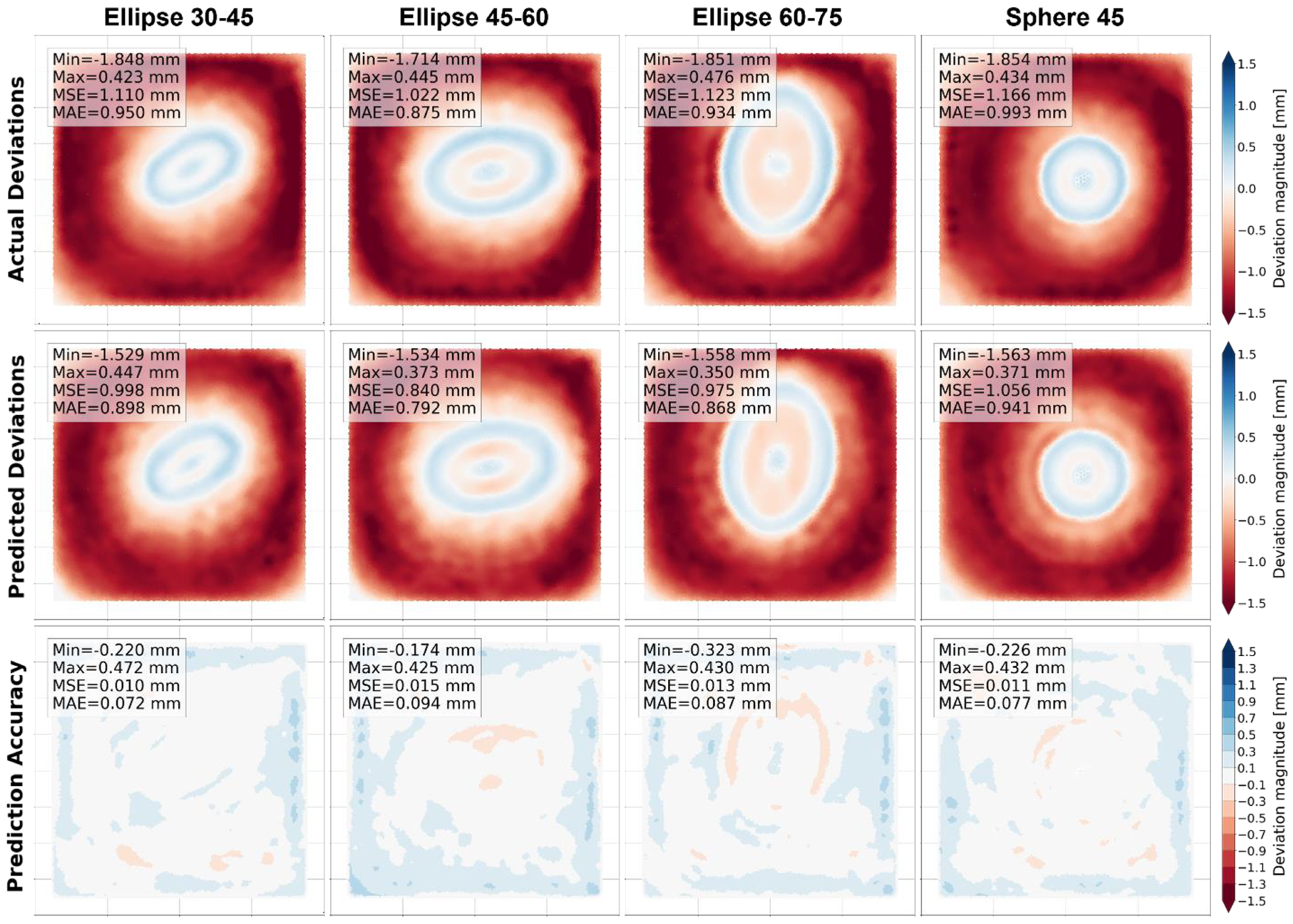
3.3. Testing Results

While the prediction of the deviations of training geometries can tell us something about the representation capabilities of the geometry-based prediction approach, the validation of the methodology is performed by making predictions for new workpieces. The main benefit of the technique will be the ability to generate compensated inputs without having to waste any material in iterative production tests.

To test the effectiveness of the method, geometry based GTB prediction was used to generate SPIF output geometries for four new derived ellipsoid workpieces. These workpieces are defined in Table 2, considering the predefined minimum and maximum workpiece parameter values. While none of the parameter combinations used for the generation of the test workpieces appears in the training dataset, the representation of these workpieces by the training data can differ. In general, the closer the resemblance of the new workpieces to the training data, the better the prediction and subsequent compensation results.

As can be seen in Figure 4, the GTB regressor was able to make good predictions for the SPIF output geometries of the test workpieces. As expected, the average MSE (0.012 mm) and MAE (0.082 mm) were both higher than for the training geometries because the regressor now encounters unknown parameter combinations. The good performance for this interpolation example, however, makes it possible for the methodology to be used as a replacement for actual production and measurement in compensation strategies.

4. Discussion

The proposed prediction method succeeds in representing the accuracy of produced parts without needing to manufacture them. The machine learning-based method implemented in a mobile workstation with a 4 GHz quad-core processor can perform the prediction for a workpiece consisting of 15,000 vertices in approximately 2 min, of which the majority of the time is used to calculate the geometric parameters. Further optimizations to the parameter calculation are possible by making use of parallelization, since normals and curvatures can be calculated completely independently for different vertices. This makes the prediction approach suitable for integration in an automated process planning procedure. There are however some limitations that need to be considered. The GTB Regressor successfully links vertex-based geometric parameters to the workpiece’s deviation behavior. The high dimensionality of the parameter vector implies that a large dataset is needed, containing a wide variety in parameter combinations, to generate a prediction model that is broadly applicable. However, for a series of similar workpiece geometries with limited variability, the prediction method can already achieve useful results with a small training data set. Another limitation is the model’s dependence on geometric information only. This means prediction results can only be used when all production parameters (materials, machines, tooling and toolpath strategies) remain fixed. For many industrial applications, this is not an immediate problem since material and tooling often remain unchanged for part production after optimization. Systematically collecting data for a growing number of produced parts, the performance of the Gradient Tree Boosting methodology can allow these to be included in a single overarching regression model, covering a widening application area.

References

1. Duflou, J.R.; Habraken, A.; Cao, J.; Malhotra, R.; Bambach, M.; Adams, D.; Vanhove, H.; Mohammadi, A.; Jeswiet, J. Single point incremental forming: State-of-the-art and prospects. Int. J. Mater. Form. 2018, 11, 743–773. [Google Scholar] [CrossRef]
2. Hirt, G.; Ames, J.; Bambach Kopp, R. Forming strategies and process modelling for CNC incremental sheet forming. CIRP Ann. 2004, 53, 203–206. [Google Scholar] [CrossRef]
3. Carette, Y.; Vanhulst, M.; Duflou, J.R. Geometry Compensation Methods for Increasing the Accuracy of the SPIF Process. Key Eng. Mater. 2021, 883, 217–224. [Google Scholar] [CrossRef]
4. Verbert, J.; Behera, A.K.; Lauwers, B.; Duflou, J.R. Multivariate adaptive regression splines as a tool to improve the accuracy of parts produced by FSPIF. Key Eng. Mater. 2011, 473, 841–846. [Google Scholar] [CrossRef]
5. Behera, A.K.; Verbert, J.; Lauwers, B.; Duflou, J.R. Tool path compensation strategies for single point incremental sheet forming using multivariate adaptive regression splines. Comput. Aided Des. 2013, 45, 575–590. [Google Scholar] [CrossRef]
6. Max, N. Weights for computing vertex normals from facet normals. J. Graph. Tools 1999, 4, 1–6. [Google Scholar] [CrossRef]
7. Theisel, H.; Rossl, C.; Zayer, R.; Seidel, H.-P. Normal Based Estimation of the Curvature Tensor for Triangular Meshes. In Proceedings of the 12th Pacific Conference on Computer Graphics and Applications, Seoul, Korea, 6–8 October 2004; pp. 288–297. [Google Scholar]
8. Friedman, J. Greedy function approximation: A gradient boosting machine. Ann. Stat. 2001, 29, 1189. [Google Scholar] [CrossRef]
9. Ke, G.; Meng, Q.; Finley, T.; Wang, T.; Chen, W.; Ma, W.; Ye, Q.; Liu, T.Y. LightGBM: A highly efficient gradient boosting decision tree. Adv. Neural Inf. Process. Syst. 2017, 30, 3146–3154. [Google Scholar]
Figure 1. Curvature based functions to determine ‘flatness’ and ‘curvedness’ for a principal curvature (L = 0.01, H = 0.02, see Equations (1) and (2)).
Engproc 26 00012 g001
Figure 2. 8 Ellipsoid training geometries determined using the fractional factorial method 2III6−3.
Engproc 26 00012 g002
Figure 3. Comparison between measured and predicted deviations and resulting prediction accuracy for four out of eight training geometries (see Table 3).
Engproc 26 00012 g003
Figure 4. Prediction of deviations of SPIF output for four new test geometries (see Table 3). Shown deviation magnitudes are calculated normal to CAD geometry.
Engproc 26 00012 g004