
Dynamic Asymmetric Causality Tests with an Application †

College of Business and Economics, UAE University, Al Ain P.O. Box 1551, United Arab Emirates
†
Presented at the 8th International Conference on Time Series and Forecasting, Gran Canaria, Spain, 27–30 June 2022.
Eng. Proc. 2022, 18(1), 41; https://doi.org/10.3390/engproc2022018041
Published: 2 August 2022
(This article belongs to the Proceedings of The 8th International Conference on Time Series and Forecasting)
Abstract
:Testing for causation—defined as the preceding impact of the past value(s) of one variable on the current value of another when all other pertinent information is accounted for—is increasingly utilized in empirical research using the time-series data in different scientific disciplines. A relatively recent extension of this approach has been allowing for potential asymmetric impacts, since this is harmonious with the way reality operates, in many cases. The current paper maintains that it is also important to account for the potential change in the parameters when asymmetric causation tests are conducted, as several reasons exist for changing the potential causal connection between the variables across time. Therefore, the current paper extends the static asymmetric causality tests by making them dynamic via the use of subsamples. An application is also provided consistent with measurable definitions of economic, or financial bad, as well as good, news and their potential causal interactions across time.
Keywords:
dynamic causality; asymmetric causality; positive changes; negative changes; oil; stock market; the USJEL Classification:
C32; C51; D82; G15; E171. Introduction
From cradle to grave, one of the most prevalent and persistent questions in life is figuring out what is the cause and what is the effect when certain pertinent events are observed. This subject must have been one of the most inspirational and important issues since the dawn of humankind. Throughout history, many philosophers have devoted their pondering to causality as an abstraction. Yet there is no common definition of causality, and above all, there is no common or universally accepted approach for detecting or measuring causality. Since the pioneer notion of [1] and the seminal contribution of [2], testing for the predictability impact of one variable on another has increasingly gained popularity and practical usefulness in different fields when the variables are quantified across time. This approach is known as Granger causality in the literature, and it describes a situation in which the past values of one variable (i.e., the cause variable) are statistically significant in an autoregressive regression model of another variable (i.e., the effect variable) when all other relevant information is also accounted for. The null hypothesis is defined as zero restrictions imposed on the parameters of the cause variable in the autoregressive model when the dependent variable is the potential effect variable. If the null hypothesis is not accepted empirically, it is taken as empirical evidence for causality, according to the Wiener–Granger method (alternative designs exist, such as those detailed by [3,4]). There have been several extensions of this method, especially since the discovery of unit roots and stochastic trends, which is a common property of many time-series variables, that quantify economic or financial processes across time. Refs. [5,6,7] suggested testing for causality via an error correction model if the variables are integrated. Ref. [8] proposed a modified [9] test statistic in order to take into account the impact of unit roots when causality tests are conducted within the vector autoregressive (VAR) model by adding additional unrestricted lags. Ref. [10,11] suggested bootstrapping with leverage adjustments in order to generate accurate critical values for the modified Wald test, since the asymptotical values are not precise when the desirable statistical assumptions for a good model are not satisfied, according to the Monte Carlo simulations conducted by the authors. The bootstrap corrected tests appear to have better size and power properties compared to the asymptotic tests, especially in small sample sizes.
However, there are numerous reasons for the potential causal connection between the variables to have an asymmetric structure. It is commonly agreed to in the literature that markets with asymmetric information prevail (based on the seminal contributions of [12,13,14]). People frequently react more strongly to a negative change, in contrast to a comparable positive one (According to [15,16,17,18], among others, there is indeed an asymmetric behavior by the investors in the financial markets, since they have a tendency to respond more strongly to negative compared to positive news). There are also natural restrictions that can lead to the asymmetric causation phenomenon. For instance, there is a limit on the potential price decrease of any normal asset or commodity, since the price cannot drop below zero. However, there is no restriction on the amount of the potential price increase. In fact, if the price decreases by a given percentage point and then increases again by the same percentage point; it will not end up at the initial price level, but at a lower level. This is true even if the process occurs in the reverse order. There are also moral and/or legal limitations that can lead to an asymmetric behavior. For example, if a company manages to increase its profit by the P% at a given period, it is feasible and easy to expand the business by that percentage point. However, if the mentioned company experiences a loss by the P%, it is not that easy to implement an immediate contraction of the business operation by the P%. The contraction is usually less than the P%, and it can take a longer time to realize this contraction compared to the corresponding expansion. It is naturally easier for the company to hire people than to fire them. In the markets for many commodities, it can also be clearly observed that there is an inertia effect for price decreases compared to price increases. Among others, the fuel market can be mentioned. When the oil price increases, there seems to be an almost immediate increase in fuel prices, and by the same proportion, if not more. However, when the oil price decreases, there is a lag in the decrease in fuel prices, and the adjustment might not be fully implemented. This indicates that the fuel prices adjustments are asymmetric with regard to the oil price changes under the ceteris paribus condition. In order to account for this kind of potential asymmetric causation in the empirical research based on time-series data, ref. [19] suggests implementing asymmetric causality tests, which the author introduces. However, these asymmetric causality tests are static by nature.
The objective of the current paper is to extend these asymmetric causality tests to a dynamic context by allowing for the underlying causal parameters to vary across time, which can be achieved by using subsamples. There are several advantages for using this dynamic parameter approach. One of the advantages of the time-varying parameter approach is that it takes into account the well-known [20] critique, which is an essential issue from the policy-making point of view. Peoples’ preferences can change across time, resulting in a change in their behavior, thereby changing the economic or financial process. There are ground-breaking technological innovations and progresses that happen with time. Major organizational restructuring can take place across time. Unexpected major events, such as the current COVID-19 pandemic, can occur. All these events can result in a change in the potential causal connection between the underlying variables in a model. Thus, a dynamic parameter model can be more informative, and it can better present the way things operate in reality. Moreover, from a correct model specification perspective, the dynamic parameter approach can be preferred to the constant parameter approach, as it is also more informative. Since the dynamic testing of the potential causation connection is more informative than the static approach, it can shed light on the extent of the pertinent phenomenon known, in the financial literature, as the correlation risk. According to [21], correlation risk is defined as the potential risk that the strength of the relationship between financial assets varies unfavorably across time. This issue can have crucial ramifications for investors, institutions, and the policy makers.
The rest of the paper is organized as follows. Section 2 introduces the methodology of dynamic asymmetric causality testing. Section 3 provides an application of the potential causal impact of oil prices on the world’s largest stock market, accounting for rising and falling prices, using both the static and the dynamic asymmetric causality tests. Conclusions are offered in the final section.
2. Dynamic Asymmetric Causality Testing
The subsequent definitions are utilized in this paper.
Definition 1.
An n-dimensional stochastic processmeasured across time is integrated of degree 1, signified as I(1), if it must be differenced once for becoming a stationary process. That is, xt ~~ I(1) if ∆xt ~~ I(0), where the denotation ∆ is the first difference operator.
Definition 2.
Defineas an n-dimensional stochastic process. Thus, during any time period, the positive and negative shocks of this random variable εt (i.e.,and) are identified as the following:
and
The definition of the positive and negative shocks was suggested by [22] for testing for hidden cointegration.
The implementation of the causality tests in the sense of the Wiener–Granger method is operational within the vector autoregressive (VAR) model of [23]. The asymmetric version of this test method is introduced by [19] (Ref. [24] extends the test to the frequency domain). Consider the following two I(1) variables with deterministic trend parts (For the simplicity of expression, we assume that n = 2. However, it is straightforward to generalize the results):
and
where a, b, c, and d are parametric constants and t is the deterministic trend term. The positive and negative partial sums of the two variables can be recursively defined as the following, based on the definitions of shocks presented in Equations (1) and (2):
where x10 and x20 are the initial values. Note that the required conditions of having and are fulfilled (For the proof of these results and for the transformation of I(2) and I(3) variables into the cumulative partial sums of negative and positive components see [25]). Interestingly, the values expressed in Equations (5)–(8) also have economic or financial implications in terms of measuring good or bad news that can affect the markets. It should be mentioned that the issue of whether to include the deterministic trends in the data generating process for a given variable is an empirical issue. In some cases, there might be the need for both a drift and a trend, and in other cases, it might be sufficient to include a drift without any trend. It is also possible to have no drift and no trend. For the selection of the deterministic trend components, the procedure suggested by [26] can be useful.
The asymmetric causality tests can be implemented via the vector autoregressive model of order p, as originally introduced by [22], i.e., the VAR(p). Let us consider testing for the potential causality between the positive components of these two variables. Then, the vector consisting of the dependent variables is defined as , and the following VAR(p) can be estimated based on this vector:
where is the 2 × 1 vector of intercepts, is a 2 × 2 matrix of parameters to be estimated for lag length r (r = 1, …, p), and is a 2 × 1 vector of the error terms. An important issue consideration before using the VAR(p) for drawing inference is to determine the optimal lag order p. This can be achieved, among other methods, by minimizing the information criterion suggested by [27], which is expressed as the following:
where is the determinant of the variance–covariance matrix of the error terms in the VAR model that is estimated based on the lag length p, ln is the natural logarithm, n is the number of time-series included in the VAR model, and T is the full sample size used for estimating the parameters in that model (The Monte Carlo simulations conducted by [28] demonstrate clearly that the information criterion expressed in equation (10) is successful in selecting the optimal lag order when the VAR model is used for forecasting purposes. In addition, the simulations show that this information criterion is robust to the ARCH effects and performs well when the variables in the VAR model are integrated. See also [29] for more information on this criterion). The lag order that results in the minimum value of the information criterion is to be selected as the optimal lag order. It is also important that the off-diagonal elements in the variance-covariance matrix are zero. Therefore, tests for multivariate autocorrelation need to be performed in order to verify this issue. The null hypothesis that the jth element of does not cause the kth element of can be tested via a [9] test statistic (It should be mentioned that the additional unrestricted lag has been added to the VAR model for taking into account the impact of one unit root, consistent with the results of [8]. Multivariate tests for autocorrelation also need to be implemented to make sure that the off-diagonal elements in the variance and covariance matrix are zero). The null hypothesis of non-causality can be formulated as the following:
For a dense representation of the Wald test statistic, we need to make use of the following denotations (It should be pointed out that this formulation requires that the p initial values for each variable in the VAR model are accessible. For the particulars on this requirement, see [30]):
as a (n × T) matrix, as a (n × (1 + n × (p + 1))) matrix, as a ((1 + n × (p + 1)) × 1) matrix, as a ((1 + n × ((p + 1) + 1)) × T) matrix and as a (n × T) matrix. Via these denotations, we can express the VAR model and the Wald test statistic compactly as the following:
The parameter matrix is estimated via the multivariate least squares as the following:
Note that and vec is the column-stacking operator. That is
The denotation is the Kronecker product operator, and C is a ((p + 1) × n) × (1 + n × (p + 1)) indicator matrix that includes one and zero elements. The restricted parameters are defined by elements of ones, and the elements of zeros are used for defining the unrestricted parameters under the null hypothesis. is an (n × n) identity matrix. represents the variance–covariance matrix of the unrestricted VAR model as expressed by Equation (12), which can be estimated as the following:
Note that the constant q represents the number of parameters that are estimated in each equation of the VAR model. By using the presented denotations, the null hypothesis of no causation might also be formulated as the following expression:
The Wald test statistic expressed in (13) that is used for testing the null hypothesis of non-causality, as defined in (11) based on the estimated VAR model in Equation (12), has the following distribution, asymptotically:
This is the case if the assumption of normality is fulfilled. Thus, the Wald test statistic for testing for potential asymmetric causal impacts has a distribution, with the number of degrees of freedom equal to the number of restrictions under the null hypothesis of non-causality, which is equal to p in this particular case. This result also holds for a corresponding VAR model for negative components, or any other combinations. For the proof, see Proposition 1 in [25].
However, if the assumption of the normal distribution of the underlying dataset is not fulfilled, the asymptotical critical values are not accurate, and bootstrap simulations need to be performed in order to obtain accurate critical values. If the variance is not constant, or if the ARCH effects prevail, then the bootstrap simulations need to be conducted with leverage adjustments. The size and power properties of the test statistics, based on the bootstrap simulation approach with leverage corrections, has been investigated by [10,11] via the Monte Carlo simulations. The simulation results provided by the previously mentioned authors show that the causality test statistic based on the leveraged bootstrapping exhibits correct size and higher power, compared to a causality test based on the asymptotic distributions, especially when the sample size is small or when the assumption of normal distribution and constant variance of the error terms are not fulfilled.
The bootstrap simulations can be conducted as the following. First, estimate the restricted model based on regression Equation (12). The restricted model imposes the restrictions under the null hypothesis of non-causality. Second, generate the bootstrap data, i.e., , via the estimated parameters from the regression, the original data, and the bootstrapped residuals. This means generating . Note that the bootstrapped residuals (i.e., ) are created by T random draws, with replacement from the modified residuals of the regression. Each of these random draws, with replacement, has the same likelihood, which is equal a probability of 1/T. The bootstrapped residuals need to be mean-adjusted in order to ensure that the residuals have zero expected value in each bootstrap sample. This is accomplished via subtracting the mean value of the bootstrap sample from each residual in that sample. Note that the residuals need to be adjusted by leverages in order to make sure that the variance is constant in each bootstrap sample. Next, repeat the bootstrap simulations 10,000 times and estimate the Wald test each time (For more information on the leverage adjustments in univariate cases, see Davison and [31], and in multivariate cases, see [10]). Use these test values in order to generate the bootstrap distribution of the test. The critical value at the α significance level via bootstrapping (denoted by ) can be acquired by taking the (α)th upper quantile of the distribution of the Wald test that is generated via the bootstrapping. The final step is to estimate the Wald test value based on the original data and compare it to the bootstrap critical value at the α level of significance. The null hypothesis of non-causation is rejected at the α significance level if the estimated Wald test value is higher than the (i.e., the bootstrap critical value at α level).
In order to account for the possibility of the potential change in the asymmetric causal connection between the variables, these tests can be conducted using subsamples. A crucial issue within this context is to determine the minimum subsample size that is required for testing for the dynamic asymmetric causality. The following formula, developed by [32], can be used for determining the smallest subsample size (S):
where T is the original full sample size. Note that S needs to be rounded up.
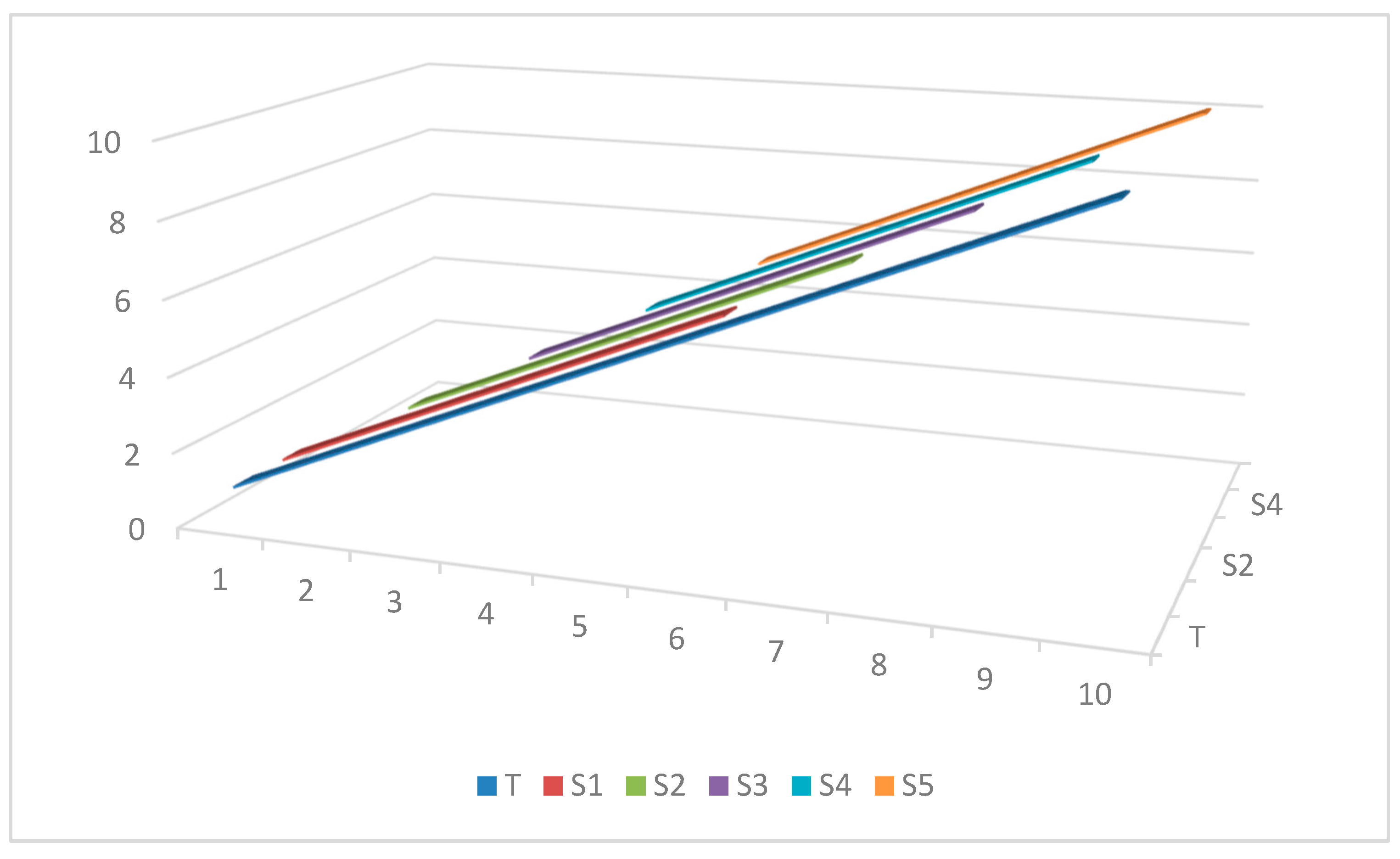
Two different approaches regarding the subsamples can be implemented for this purpose. The first one is the fixed rolling window approach, which is based on repeated estimation of the model, with a subsample size of S each time, and the window is moved forward by one observation each time. That is, we need to estimate the time varying causality for the following subsamples, where each number represents a point in time:
This means that the first subsample consists of the range covering the first observation to the S observation. The next subsample removes the first observation from S and adds the one after S. The process is continued until the full range is covered. For example, assume that T = 10 and then we have S = 6 based on Equation (19) when S is rounded up (Obviously, the sample size normally needs to be bigger than 10 observations in the empirical analysis. Here, a very small sample size is assumed for the sake of the simplicity of the expression). Thus, we have the following subsamples (where each number represents the corresponding time):
The graphical illustration of this approach for the current example is depicted in Figure 1.
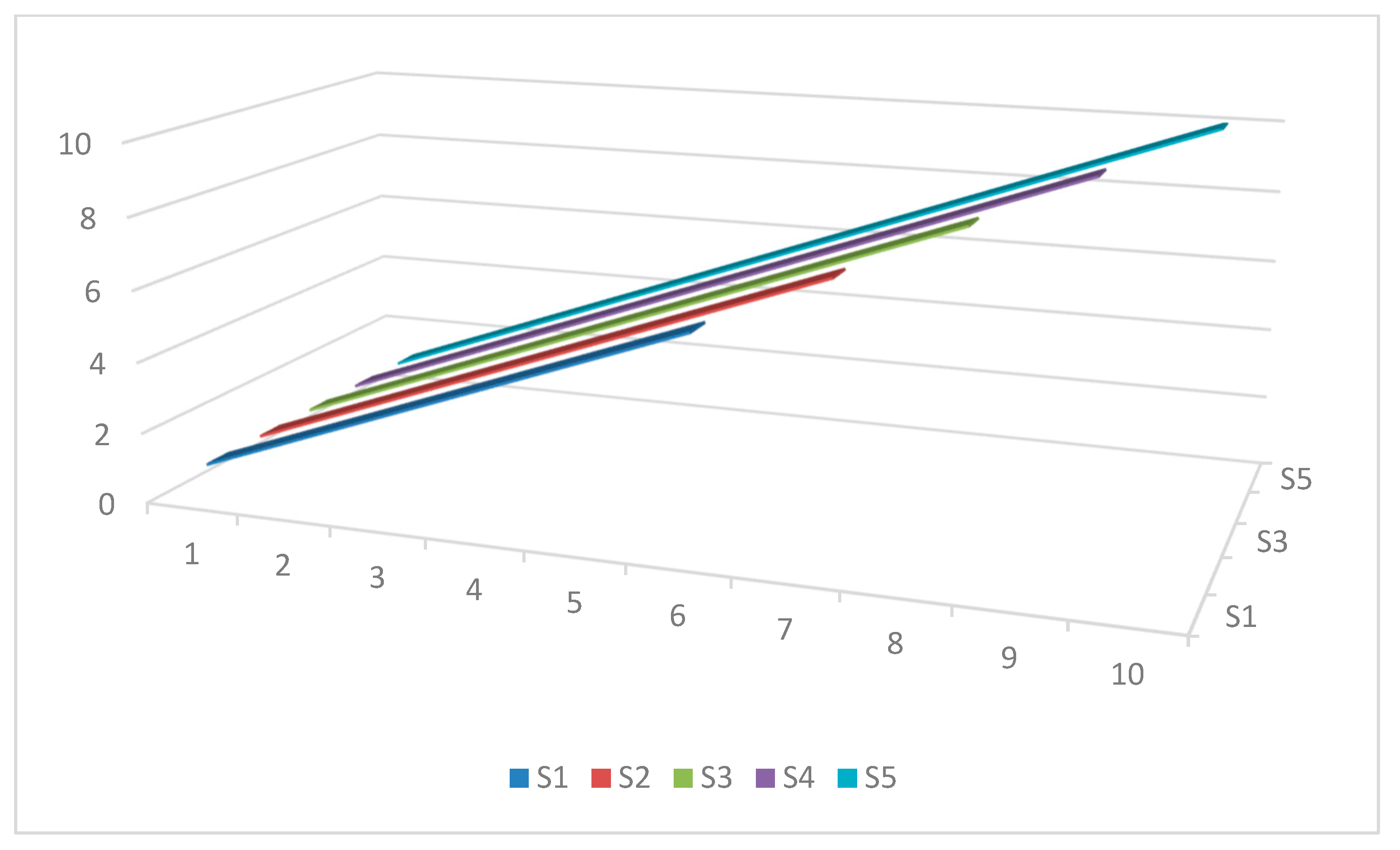
The second method for determining multiple subsamples is to start with S and recursively add an observation to S each time for obtaining the next subsample without removing any observation from the beginning. In this approach, the sample size increases by one observation in each subsample until it covers the full range. That is, the size of the first subsample is equal to S and the size of the last one is equal to T. This is a recursive rolling window approach that is anchored at the start. The graphical drawing of this method for the mentioned example is shown in Figure 2.
The next step in order to implement the dynamic asymmetric causality tests is to calculate the Wald test statistic for each subsample and produce its bootstrap critical value at a given significance level. Then, the following ratio can be calculated for each subsample:
where TVpCV signifies the test value per the critical value at a given significance level using a particular subsample. If this ratio is higher than one, it implies that the null hypothesis of no causality is rejected at the given significance level for that subsample. The 5% and the 10% significance levels can be considered. A graphical illustration of (20) for different subsamples can be informative to the investigator in order to detect the potential change of the asymmetric causal connection between the underlying variables in the model.
An alternative method for estimating and testing the time-varying asymmetric causality tests is to make use of the [33] filter within a multivariate setting. However, this method might not be operational if the dimension of the model is rather high and/or the lag order is large.
3. An Application
An application is provided for detecting the change in the potential causal impact of oil prices and the world’s largest financial market. Two indexes are used for this purpose. The first one is the total share prices index for all shares for the US. The second index is the global price of Brent Crude in USD per barrel. The frequency of the data is yearly, and it covers the period of 1990–2020. The source of the data is the FRED database, which is provided by the Federal Reserve Bank of St. Louis. Let us denote the stock price index by S and the oil price index by O. The aim of this application is to investigate whether the potential impact of rising or falling oil prices on the performance of the world’s largest stock market is time dependent or not. Interestingly, the US market is not only the largest market and its financial market is the most valuable in the word, but the US is also the biggest oil producer in the world. These combinations might make the empirical results of this pragmatic application more useful and general.
The variables are expressed in the natural logarithm format. The unit root test results of the conducted Phillips–Perron test confirm that each variable is integrated at the first order (The unit root test results are not reported, but they are available on request). First, the following linear regression is estimated via the OLS technique for the stock price index (i.e., ):
Next, the residuals of the above regression are estimated. That is
Note that the circumflex implies the estimated value. The positive and negative shocks are measured as the following, based on the definitions presented in Equations (1) and (2):
The positive and negative partial sums for this variable are defined as the following, based on the results presented in Equations (5) and (6):
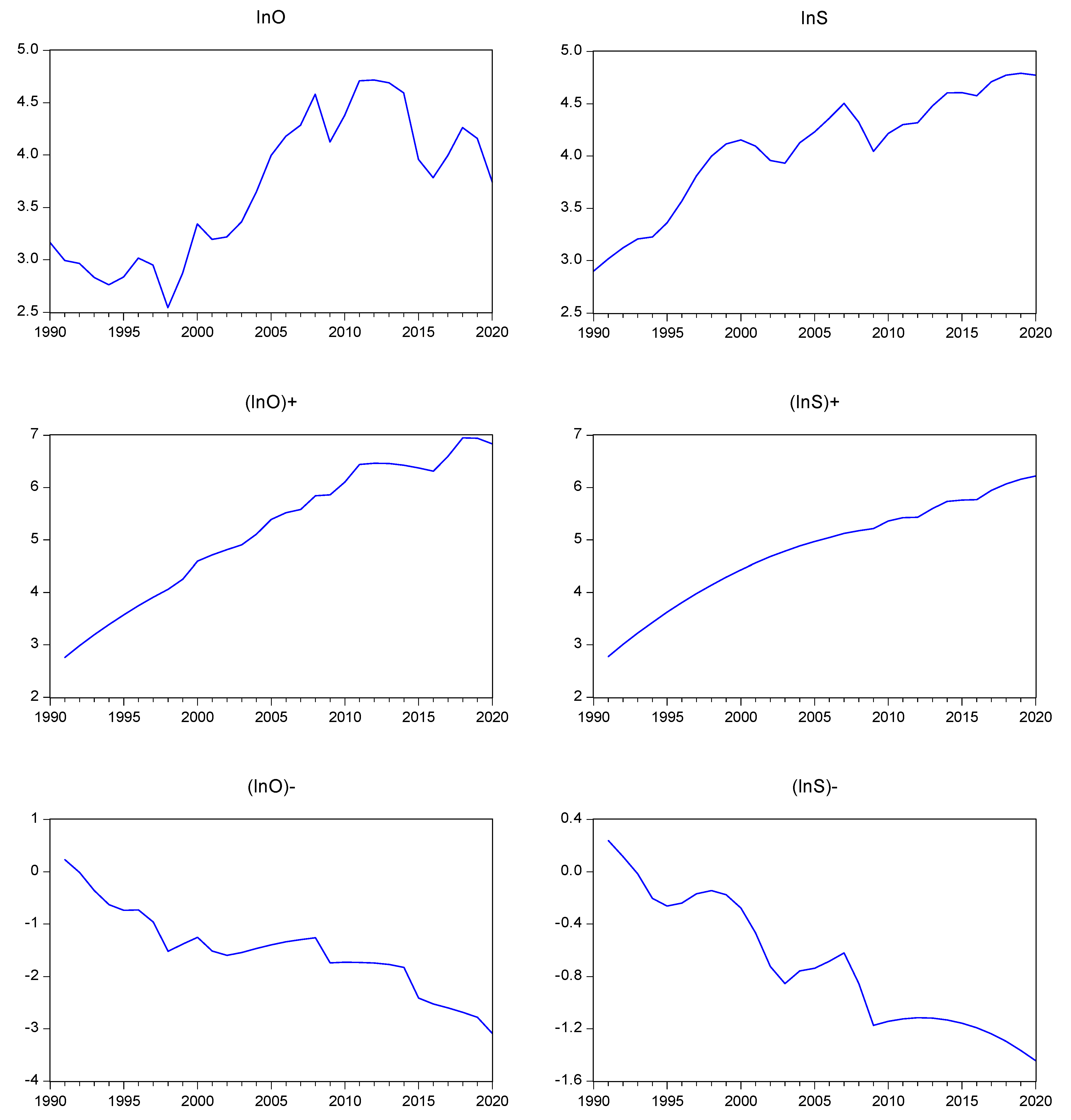
where signifies the initial value of the stock price index in the logarithmic format, which is assumed to be zero, in this case. Note that the equivalency condition is fulfilled. It should be mentioned that the value expressed by Equation (22) represents the good news with regard to the stock market, while the value expressed by Equation (23) signifies the bad news pertaining to the same market. The oil price index can also be transformed into cumulative partial sums of positive and negative components in an analogous way. Note that a drift and a trend were included in the equation of each variable, since it seems to be needed, based on the graphs presented in Figure 3.
The dataset can be transformed by a number of user-friendly statistical software components. Prior to implementing causality tests, diagnostic tests were also implemented. The results of these tests are presented in Table A1, which indicate that the assumption of normality is not fulfilled, and the conditional variance is not constant, in most cases. Thus, making use of the bootstrap simulations with leverage adjustments is necessary in order to produce reliable critical values. This is particularly the case for subsamples, since the degrees of freedom are lower.
Both symmetric and the asymmetric causality tests are implemented in a dynamic setting using the statistical software component created by [34] in Gauss. The results for the symmetric causality tests are presented in Table A2 and Table A3, based on the 5% and the 10% significance levels. Based on these results, it can be inferred that the oil price does not cause the results of the stock market price index, not even at the 10% significance level.
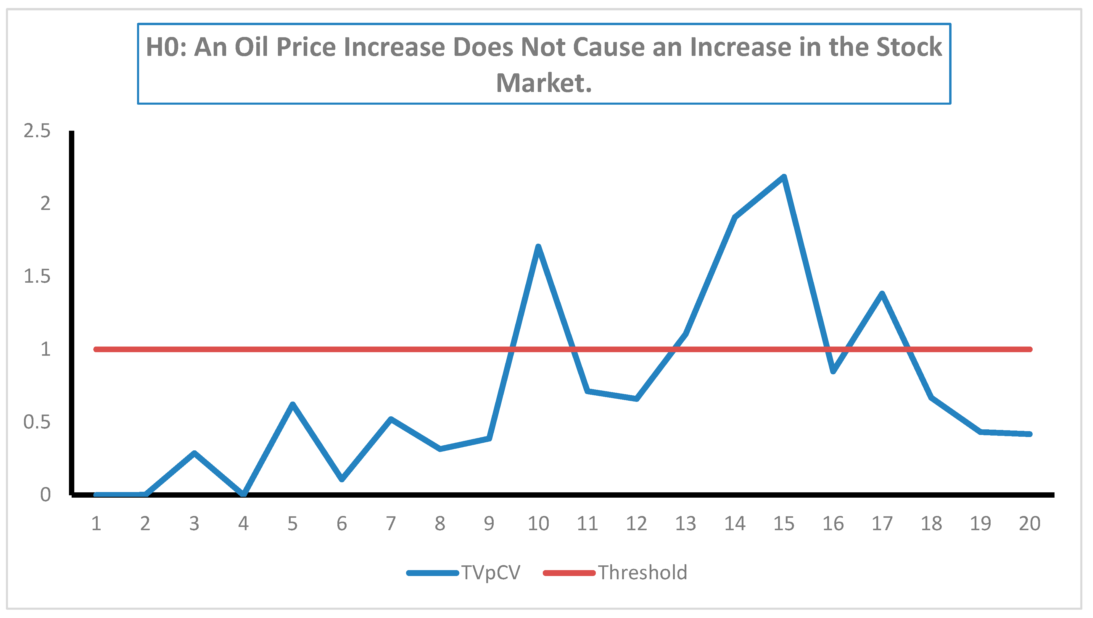
The results are also robust regarding the choice of the subsamples because the same results are obtained with all subsamples. An implication of this empirical finding is that the market is informationally efficient in the semi-strong form with regard to oil prices, as defined by [35]. However, when the tests for dynamic asymmetric causality are implemented, the results show that an oil price decrease does not cause a decrease in the stock market price index, and these results are the same across subsamples, even at the 10% significance level (see Table A4, Table A5 and Table A6). Conversely, the null hypothesis that an oil price increase does not cause an increase in the stock market price index is rejected during four subsamples.
4. Conclusions
Tests for causality in the Wiener–Granger method are regularly used in empirical research regarding the time series data in different scientific disciplines. A popular extension of this approach is the asymmetric casualty testing approach, as developed by Hatemi-J (2012). However, this approach is static by nature. A pertinent issue within this context is whether the potential asymmetric causal impacts between the underlying variables in a model are steady or not over the selected time span. In order to throw light on this issue, the current paper suggests implementing asymmetric causality tests across time to see whether the potential asymmetric causal impact is time dependent or not. This can be achieved by using subsamples via two different approaches.
An application is provided in order to investigate the potential causal connection of oil prices with the stock prices of the world’s largest financial market within a time-varying setting. The results of the dynamic symmetric causality tests show that the oil prices do not cause the level of the market price index, regardless of the subsample size. However, when the dynamic asymmetric causality tests are implemented, the results show that positive oil price changes cause a positive price change in the stock market using certain subsamples. In fact, if only three fewer observations are used compared to the full sample size, the results show that there is causality from the oil price increase to the stock market price increase. Conversely, if the full sample size is used (i.e., only three more degrees of freedom), no causality is found. This shows that it can indeed be important to make use of the dynamic causality tests in order to see whether or not the causality result is robust across time.
It should be pointed out that an alternative method for estimating and testing the time-varying asymmetric causality tests is to make use of the [33] filter within a multivariate setting. However, this method might not be operational if the dimension of the VAR model is rather high and/or the lag order is large.
The time-varying asymmetric causality tests results can shed light on whether the causal connection between the variables of interest is general or time dependent. This has important practical implications. If the causal connection changes across time, then the decision or policy based on this causal impact needs to be time dependent as well. This is the case because a static strategy is likely to be inefficient within a dynamic environment.
At the end, the following English proverb that has been quoted by Wiener (1956) [1] says it all.
“For want of a nail, the shoe was lost;For want of a shoe, the horse was lost;For want of a horse, the rider was lost;For want of a rider, the battle was lost;For want of a battle, the kingdom was lost!”
Funding
This research received no external funding.
Institutional Review Board Statement
Not applicable.
Informed Consent Statement
Not applicable.
Data Availability Statement
FRED DATA BASE, https://fred.stlouisfed.org (accessed on 26 June 2021).
Acknowledgments
This paper was presented at the 8th International Conference on Time Series and Forecasting (ITISE 2022), Spain. The author would like to thank the participants for their comments. The usual disclaimer applies, nevertheless.
Conflicts of Interest
The author declares no conflict of interest.
Appendix A

Table A1.
Test results for multivariate normality and multivariate ARCH in the VAR model.
| Variables in the Model | The p-Values of the Multivariate Normality Tests | The p-Values of the Multivariate ARCH Tests |
|---|---|---|
| 0.0814 | 0.3743 | |
| 0.5555 | 0.0028 | |
| 0.0087 | 0.0150 |
Notes: (1) lnOt signifies the oil price index and lnSt indicates the US stock price index for all shares. The vector denotes the cumulative partial sum of the positive changes, and the vector indicates the cumulative partial sum of the negative changes. (2) The multivariate test of [36] was implemented for testing the null hypothesis of multivariate normality in the residuals in each VAR model. (3) The multivariate test of [37] was conducted for testing the null hypothesis of no multivariate ARCH (1).
Table A2.
Dynamic symmetric causality test results at the 5% significance level. (H0: The oil price does not cause the stock market price index).
Table A2.
Dynamic symmetric causality test results at the 5% significance level. (H0: The oil price does not cause the stock market price index).
| SSP | Test Value | 10% Bootstrap CV | TVpCV |
|---|---|---|---|
| 1 | 1.788 | 572.528 | 0 |
| 2 | 1.431 | 52.787 | 0.034 |
| 3 | 0.832 | 20.977 | 0.068 |
| 4 | 0.863 | 13.312 | 0.062 |
| 5 | 0.112 | 10.484 | 0.082 |
| 6 | 0.317 | 4.592 | 0.024 |
| 7 | 0.365 | 5.385 | 0.059 |
| 8 | 0.429 | 5.135 | 0.071 |
| 9 | 0.239 | 4.678 | 0.092 |
| 10 | 0.525 | 4.502 | 0.053 |
| 11 | 0.5 | 4.76 | 0.11 |
| 12 | 0.538 | 4.054 | 0.123 |
| 13 | 0.642 | 4.561 | 0.118 |
| 14 | 0.757 | 4.606 | 0.139 |
| 15 | 0.591 | 4.859 | 0.156 |
| 16 | 0.281 | 4.211 | 0.14 |
| 17 | 0.623 | 3.68 | 0.076 |
| 18 | 0.635 | 4.571 | 0.136 |
| 19 | 0.638 | 4.252 | 0.149 |
| 20 | 0.627 | 4.403 | 0.145 |
| 21 | 0.627 | 4.129 | 0.152 |
DENOTATIONS: SSP: The subsample period. CV: the critical value; TVpCV: the test value per the critical value; TVpCV = (test value)/(bootstrap critical value at the given significance level). If the value of TVpCV > 1, it implies that the null hypothesis of no causality is rejected at the given significance level.
Table A3.
Dynamic symmetric causality test results at the 10% significance level. (H0: The oil price does not cause the stock market price index).
Table A3.
Dynamic symmetric causality test results at the 10% significance level. (H0: The oil price does not cause the stock market price index).
| SSP | Test Value | 10% Bootstrap CV | TVpCV |
|---|---|---|---|
| 1 | 0.187 | 139.42 | 0.001 |
| 2 | 1.788 | 22.105 | 0.081 |
| 3 | 1.431 | 10.186 | 0.14 |
| 4 | 0.832 | 8.851 | 0.094 |
| 5 | 0.863 | 7.811 | 0.11 |
| 6 | 0.112 | 2.957 | 0.038 |
| 7 | 0.317 | 3.574 | 0.089 |
| 8 | 0.365 | 3.231 | 0.113 |
| 9 | 0.429 | 3.188 | 0.135 |
| 10 | 0.239 | 3.043 | 0.079 |
| 11 | 0.525 | 3.011 | 0.174 |
| 12 | 0.5 | 2.876 | 0.174 |
| 13 | 0.538 | 3.083 | 0.174 |
| 14 | 0.642 | 2.95 | 0.218 |
| 15 | 0.757 | 3.218 | 0.235 |
| 16 | 0.591 | 2.835 | 0.209 |
| 17 | 0.281 | 2.623 | 0.107 |
| 18 | 0.623 | 3.04 | 0.205 |
| 19 | 0.635 | 2.894 | 0.219 |
| 20 | 0.638 | 2.981 | 0.214 |
| 21 | 0.627 | 3.05 | 0.206 |
DENOTATIONS: SSP: the subsample period; CV: the critical value; TVpCV: the test value per the critical value; TVpCV = (test value)/(bootstrap critical value at the given significance level). If the value of TVpCV > 1, it implies that the null hypothesis of no causality is rejected at the given significance level.
Table A4.
Dynamic asymmetric causality test results at the 10% significance level. (H0: An oil price increase does not cause an increase in the stock market price index).
Table A4.
Dynamic asymmetric causality test results at the 10% significance level. (H0: An oil price increase does not cause an increase in the stock market price index).
| SSP | Test Value | 10% Bootstrap CV | TVpCV |
|---|---|---|---|
| 1 | 0 | 0.104 | 0 |
| 2 | 0 | 0 | 0.001 |
| 3 | 0.003 | 0.01 | 0.287 |
| 4 | 0 | 10.351 | 0 |
| 5 | 5.292 | 8.517 | 0.621 |
| 6 | 0.838 | 7.86 | 0.107 |
| 7 | 2.89 | 5.562 | 0.52 |
| 8 | 1.052 | 3.335 | 0.315 |
| 9 | 1.124 | 2.905 | 0.387 |
| 10 | 10.014 | 5.873 | 1.705 |
| 11 | 2.309 | 3.245 | 0.712 |
| 12 | 3.688 | 5.594 | 0.659 |
| 13 | 6.353 | 5.749 | 1.105 |
| 14 | 9.888 | 5.188 | 1.906 |
| 15 | 11.778 | 5.392 | 2.184 |
| 16 | 2.607 | 3.074 | 0.848 |
| 17 | 7.435 | 5.378 | 1.382 |
| 18 | 2.136 | 3.2 | 0.667 |
| 19 | 1.279 | 2.965 | 0.432 |
| 20 | 1.288 | 3.085 | 0.417 |
DENOTATIONS: SSP: the subsample period; CV: the critical value; TVpCV: the test value per the critical value; TVpCV = (test value)/(bootstrap critical value at the given significance level). If the value of TVpCV > 1, it implies that the null hypothesis of no causality is rejected at the given significance level.
Table A5.
Dynamic asymmetric causality test results at the 5% significance level. (H0: An oil price decrease does not cause a decrease in the stock market price index).
Table A5.
Dynamic asymmetric causality test results at the 5% significance level. (H0: An oil price decrease does not cause a decrease in the stock market price index).
| SSP | Test Value | 10% Bootstrap CV | TVpCV |
|---|---|---|---|
| 1 | 40.802 | 415.432 | 0.098 |
| 2 | 1.021 | 34.228 | 0.030 |
| 3 | 1.001 | 19.468 | 0.051 |
| 4 | 1.245 | 14.706 | 0.085 |
| 5 | 0.44 | 11.328 | 0.039 |
| 6 | 0.525 | 9.4 | 0.056 |
| 7 | 0.616 | 10.372 | 0.059 |
| 8 | 0.036 | 5.526 | 0.007 |
| 9 | 0 | 5.221 | 0 |
| 10 | 0.353 | 4.948 | 0.071 |
| 11 | 0.362 | 4.86 | 0.075 |
| 12 | 0.373 | 4.692 | 0.080 |
| 13 | 0.382 | 4.387 | 0.087 |
| 14 | 0.387 | 4.717 | 0.082 |
| 15 | 0.372 | 4.664 | 0.080 |
| 16 | 0.081 | 4.374 | 0.019 |
| 17 | 0.085 | 4.338 | 0.020 |
| 18 | 0.087 | 5.029 | 0.017 |
| 19 | 0.084 | 4.757 | 0.018 |
| 20 | 0.078 | 4.499 | 0.017 |
DENOTATIONS: SSP: the subsample period; CV: the critical value; TVpCV: the test value per the critical value; TVpCV = (test value)/(bootstrap critical value at the given significance level). If the value of TVpCV > 1, it implies that the null hypothesis of no causality is rejected at the given significance level.
Table A6.
Dynamic asymmetric causality test results at the 10% significance level. (H0: An oil price decrease does not cause a decrease in the stock market price index).
Table A6.
Dynamic asymmetric causality test results at the 10% significance level. (H0: An oil price decrease does not cause a decrease in the stock market price index).
| SSP | Test Value | 10% Bootstrap CV | TVpCV |
|---|---|---|---|
| 1 | 40.802 | 93.964 | 0.434 |
| 2 | 1.021 | 19.269 | 0.053 |
| 3 | 1.001 | 10.783 | 0.093 |
| 4 | 1.245 | 9.204 | 0.135 |
| 5 | 0.44 | 7.935 | 0.055 |
| 6 | 0.525 | 6.316 | 0.083 |
| 7 | 0.616 | 6.836 | 0.09 |
| 8 | 0.036 | 3.601 | 0.01 |
| 9 | 0 | 3.339 | 0 |
| 10 | 0.353 | 3.275 | 0.108 |
| 11 | 0.362 | 3.048 | 0.119 |
| 12 | 0.373 | 3.248 | 0.115 |
| 13 | 0.382 | 3.076 | 0.124 |
| 14 | 0.387 | 3.199 | 0.121 |
| 15 | 0.372 | 2.938 | 0.127 |
| 16 | 0.081 | 2.862 | 0.028 |
| 17 | 0.085 | 2.784 | 0.031 |
| 18 | 0.087 | 3.205 | 0.027 |
| 19 | 0.084 | 2.884 | 0.029 |
| 20 | 0.078 | 3.066 | 0.025 |
DENOTATIONS: SSP: the subsample period; CV: the critical value; TVpCV: the test value per the critical value; TVpCV = (test value)/(bootstrap critical value at the given significance level). If the value of TVpCV > 1, it implies that the null hypothesis of no causality is rejected at the given significance level.
Table A7.
Dynamic asymmetric causality test results at the 5% significance level. (H0: An oil price increase does not cause an increase in the stock market price index.).
Table A7.
Dynamic asymmetric causality test results at the 5% significance level. (H0: An oil price increase does not cause an increase in the stock market price index.).
| SSP | Test Value | 5% Bootstrap CV | TVpCV |
|---|---|---|---|
| 1 | 0 | 0.157 | 0 |
| 2 | 0 | 0 | 0 |
| 3 | 0.003 | 0.039 | 0.072 |
| 4 | 0 | 16.548 | 0 |
| 5 | 5.292 | 12.61 | 0.42 |
| 6 | 0.838 | 11.836 | 0.071 |
| 7 | 2.89 | 8.299 | 0.348 |
| 8 | 1.052 | 5.009 | 0.21 |
| 9 | 1.124 | 4.334 | 0.259 |
| 10 | 10.014 | 8.446 | 1.186 |
| 11 | 2.309 | 4.543 | 0.508 |
| 12 | 3.688 | 7.523 | 0.49 |
| 13 | 6.353 | 7.967 | 0.797 |
| 14 | 9.888 | 7.387 | 1.339 |
| 15 | 11.778 | 7.529 | 1.564 |
| 16 | 2.607 | 5.282 | 0.494 |
| 17 | 7.435 | 7.514 | 0.989 |
| 18 | 2.136 | 4.334 | 0.493 |
| 19 | 1.279 | 4.311 | 0.297 |
| 20 | 1.288 | 4.536 | 0.284 |
DENOTATIONS: SSP: the subsample period; CV: the critical value; TVpCV: the test value per the critical value; TVpCV (test value)/(bootstrap critical value at the given significance level). If the value of TVpCV > 1, it implies that the null hypothesis of no causality is rejected at the given significance level.
References
- Wiener, N. The Theory of Prediction. In Modern Mathematics for Engineers; Beckenbach, E.F., Ed.; McGraw-Hill: New York, NY, USA, 1956; Volume 1. [Google Scholar]
- Granger, C.W. Investigating Causal Relations by Econometric Models and Cross-spectral methods. Econometrica 1969, 37, 424–439. [Google Scholar] [CrossRef]
- Sims, C.A. Money, Income and Causality. Am. Econ. Rev. 1972, 62, 540–552. [Google Scholar]
- Geweke, J. Measurement of Linear Dependence and Feedback between Multiple Time Series. J. Am. Stat. Assoc. 1982, 77, 304–324. [Google Scholar] [CrossRef]
- Granger, C.W. Developments in the Study of Cointegrated Economic Variables. Oxf. Bull. Econ. Stat. 1986, 48, 213–228. [Google Scholar] [CrossRef]
- Granger, C.W. Some Recent Development in a Concept of Causality. J. Econom. 1988, 39, 199–211. [Google Scholar] [CrossRef]
- Engle, R.F.; Granger, C.W. Co-integration and error correction: Representation, estimation, and testing. Econometrica 1987, 55, 251–276. [Google Scholar] [CrossRef]
- Toda, H.Y.; Yamamoto, T. Statistical Inference in Vector Autoregressions with Possibly Integrated Processes. J. Econom. 1995, 66, 225–250. [Google Scholar] [CrossRef]
- Wald, A. Contributions to the Theory of Statistical Estimation and Testing Hypotheses. Ann. Math. Stat. 1939, 10, 299–326. [Google Scholar] [CrossRef]
- Hacker, S.; Hatemi-J, A. Tests for Causality between Integrated Variables using Asymptotic and Bootstrap Distributions: Theory and Application. Appl. Econ. 2006, 38, 1489–1500. [Google Scholar] [CrossRef]
- Hacker, S.; Hatemi-J, A. A Bootstrap Test for Causality with Endogenous Lag Length Choice: Theory and Application in Finance. J. Econ. Stud. 2012, 39, 144–160. [Google Scholar] [CrossRef] [Green Version]
- Akerlof, G. The Market for Lemons: Quality Uncertainty and the Market Mechanism. Q. J. Econ. 1970, 84, 488–500. [Google Scholar] [CrossRef]
- Spence, M. Job Market Signalling. Q. J. Econ. 1973, 87, 355–374. [Google Scholar] [CrossRef]
- Stiglitz, J. Incentives and Risk Sharing in Sharecropping. Rev. Econ. Stud. 1974, 41, 219–255. [Google Scholar] [CrossRef] [Green Version]
- Longin, F.; Solnik, B. Extreme correlation of international equity markets. J. Financ. 2001, 56, 649–676. [Google Scholar] [CrossRef]
- Ang, A.; Chen, J. Asymmetric correlations of equity portfolios. J. Financ. Econ. 2002, 63, 443–494. [Google Scholar] [CrossRef]
- Hong, Y.; Zhou, G. Asymmetries in stock returns: Statistical test and economic evaluation. Rev. Financ. Stud. 2008, 20, 1547–1581. [Google Scholar] [CrossRef]
- Alvarez-Ramirez, J.; Rodriguez, E.; Echeverria, J.C. A DFA approach for assessing asymmetric correlations. Phys. A Stat. Mech. Its Appl. 2009, 388, 2263–2270. [Google Scholar] [CrossRef]
- Hatemi-J, A. Asymmetric Causality Tests with an Application. Empir. Econ. 2012, 43, 447–456. [Google Scholar] [CrossRef]
- Lucas, R.E. Econometric Policy Evaluation: A Critique. In The Phillips Curve and Labor Markets. Carnegie-Rochester Conference Series on Public Policy; Brunner, K., Meltzer, A., Eds.; Elsevier: New York, NY, USA, 1976; Volume 1, pp. 19–46. [Google Scholar]
- Meissner, G. Correlation Risk Modelling and Management; Wiley Financial Series; Wiley: Hoboken, NJ, USA, 2014. [Google Scholar]
- Granger, C.W.; Yoon, G. Hidden Cointegration; Department of Economics Working Paper; University of California: San Diego, CA, USA, 2002. [Google Scholar]
- Sims, C.A. Macroeconomics and Reality. Econometrica 1980, 48, 1–48. [Google Scholar] [CrossRef] [Green Version]
- Bahmani-Oskooee, M.; Chang, T.; Ranjbarc, O. Asymmetric causality using frequency domain and time-frequency domain (wavelet) approaches. Econ. Model. 2016, 56, 66–78. [Google Scholar] [CrossRef]
- Hatemi-J, A.; El-Khatib, Y. An Extension of the Asymmetric Causality Tests for Dealing with Deterministic Trend Components. Appl. Econ. 2016, 48, 4033–4041. [Google Scholar] [CrossRef]
- Hacker, S.; Hatemi-J, A. The Properties of Procedures Dealing with Uncertainty about Intercept and Deterministic Trend in Unit Root Testing; Working Paper Series in Economics and Institutions of Innovation 214; Royal Institute of Technology, CESIS—Centre of Excellence for Science and Innovation Studies: Stockholm, Sweden, 2010. [Google Scholar]
- Hatemi-J, A. A new method to choose optimal lag order in stable and unstable VAR models. Appl. Econ. Lett. 2003, 10, 135–137. [Google Scholar] [CrossRef]
- Hatemi-J, A. Forecasting properties of a new method to choose optimal lag order instable and unstable VAR models. Appl. Econ. Lett. 2008, 15, 239–243. [Google Scholar] [CrossRef]
- Mustafa, A.; Hatemi-J, A. A VBA Module Simulation for Finding Optimal Lag Order in Time Series Models and Its Use on Teaching Financial Data Computation. Appl. Comput. Inform. 2022, 18, 208–220. [Google Scholar] [CrossRef]
- Lutkepohl, H. New Introduction to Multiple Time Series Analysis; Springer: Berlin/Heidelberg, Germany, 2005. [Google Scholar]
- Davison, A.C.; Hinkley, D.V. Bootstrap Methods and Their Application; Cambridge University Press: Cambridge, UK, 1999. [Google Scholar]
- Phillips, P.C.; Shi, S.; Yu, J. Testing for multiple bubbles: Historical episodes of exuberance and collapse in the S&P 500. Int. Econ. Rev. 2015, 56, 1043–1078. [Google Scholar]
- Kalman, R.E. A New Approach to Linear Filtering and Prediction Problems. J. Basic Eng. 1960, 82, 35–45. [Google Scholar] [CrossRef] [Green Version]
- Hatemi-J, A.; Mustafa, A. DASCT01: Gauss Module for estimating Dynamic Asymmetric and Symmetric Causality Tests, Statistical Software Components D00001, Boston College Department of Economics. 2021. Available online: https://ideas.repec.org/c/boc/bocode/d00001.html (accessed on 11 May 2021).
- Fama, E.F. Efficient Capital Markets: A Review of Theory and Empirical Work. J. Financ. 1970, 25, 383–417. [Google Scholar] [CrossRef]
- Doornik, J.A.; Hansen, H. An omnibus test for univariate and multivariate normality. Oxf. Bull. Econ. Stat. 2008, 70, 927–939. [Google Scholar] [CrossRef]
- Hacker, S.; Hatemi-J, A. A multivariate test for ARCH effects. Appl. Econ. Lett. 2005, 12, 411–417. [Google Scholar] [CrossRef]
Figure 1.
The illustration of the subsamples compared to the entire sample based on the fixed rolling window approach. Notes: T represents the full sample size, and Si represents subsample i (for i = 1, …, 5.), in this case.
Figure 1.
The illustration of the subsamples compared to the entire sample based on the fixed rolling window approach. Notes: T represents the full sample size, and Si represents subsample i (for i = 1, …, 5.), in this case.

Figure 2.
The graphical presentation of the subsamples based on the recursive rolling window approach. Notes: Si represents subsample i (for i = 1, …, 5.), in this example. Note that the S5 = T, in this case.
Figure 2.
The graphical presentation of the subsamples based on the recursive rolling window approach. Notes: Si represents subsample i (for i = 1, …, 5.), in this example. Note that the S5 = T, in this case.

Figure 3.
The time plot of the variables, along with the cumulative partial components for positive and negative parts. Notes: The notation lnOt represents the oil price index, and lnSt represents the US stock market price index for all shares. The corresponding sign indicates the positive and negative components.

Figure 4.
The time plot of the causality test results for the positive components at the 10% significance level.
Figure 4.
The time plot of the causality test results for the positive components at the 10% significance level.

Publisher’s Note: MDPI stays neutral with regard to jurisdictional claims in published maps and institutional affiliations. |
© 2022 by the author. Licensee MDPI, Basel, Switzerland. This article is an open access article distributed under the terms and conditions of the Creative Commons Attribution (CC BY) license (https://creativecommons.org/licenses/by/4.0/).
Share and Cite
MDPI and ACS Style
Hatemi-J, A. Dynamic Asymmetric Causality Tests with an Application. Eng. Proc. 2022, 18, 41. https://doi.org/10.3390/engproc2022018041
AMA Style
Hatemi-J A. Dynamic Asymmetric Causality Tests with an Application. Engineering Proceedings. 2022; 18(1):41. https://doi.org/10.3390/engproc2022018041
Chicago/Turabian StyleHatemi-J, Abdulnasser. 2022. "Dynamic Asymmetric Causality Tests with an Application" Engineering Proceedings 18, no. 1: 41. https://doi.org/10.3390/engproc2022018041