Using Forecasting Methods on Crime Data: The SKALA Approach of the State Office for Criminal Investigation of North Rhine-Westphalia ^†

Abstract

In this article, we introduce the topic of crime forecasting performed in North Rhine-Westphalia, Germany. We give a brief overview of three forecasting methods used in theory and practice: predictive policing, risk terrain modeling, and time series analysis. As a result, spatio-temporally-based statistical techniques offered high potential to optimize operational and strategic planning for policing.

1. Introduction

Crime is a complex social phenomenon that has a lasting impact on the population’s sense of security and can burden society. The complexity of this phenomenon makes it difficult to predict. Every day, new crimes of different types occur because of different decisions and the routine activities of perpetrators, victims, and capable guardians, resulting in many new trends in crime. Investigating these crime characteristics, crime patterns, and criminal behavior is a major objective of criminology. In the last decades, many new options in criminal investigation have arisen as a result of rapid technological development and newly designed technologies. Because of the difficulty in dealing with the massive amount of data produced every day, data mining techniques have also become increasingly crucial in terms of criminal investigation. The digitalization of society also led to the development of different policing strategies and philosophies, which are often based on extensive data systems (Big Data). In addition, the importance of system-related decision-making processes in policing increases [1]. Nowadays, in the investigation, prosecution, and prevention of crime, crime analysis and the use of big data play a significant role.

Attempting to anticipate the future is not a new way of thinking in the context of policing, but rather a standard approach. For example, prevention efforts—which are a foremost task of the police—aim to prevent potential future threats in a pre-emptive manner. Two insights are essential for the idea of crime forecasting: First, human actions can vary due to different values and preferences and also due to the influence of spatial/temporal changes [2]; and second, crimes do not occur uniformly or randomly in space and time [3] (p. 5). What is new is the systematic use of technical solutions, big data, and the gaining complexity of data analytics in policing. With the police trying to explore what they might already know based on their existing data, police open the door to using big data and linking data to intelligence. In this spirit of optimism, a wide variety of data analysis methods have been implemented in German police forces since 2014. These include methods such as predictive policing. The State Office for Criminal Investigation of North Rhine-Westphalia (LKA NRW) tested and implemented its own predictive policing model as part of a holistic crime analysis and forecasting approach, called SKALA (System for Crime Analysis and Anticipation). The SKALA approach intends to understand the main use of crime analysis and forecast algorithms, such as predictive policing methods, risk terrain modeling, and time series analysis, to investigate crime patterns at different spatial and temporal scales to support crime prevention. Currently, the focus is on residential burglaries, commercial burglaries, and motor vehicle offenses. This is because numerous theoretical and empirical scientific works are already available both on the phenomenology and explanation of these particular offenses and on the distribution of crime phenomena in space and time. These formed an essential cornerstone for the conception and evaluation of the models and of the forecast development.

This paper gives an overview of the different methods used to forecast crimes in the context of SKALA. The crime-forecasting project in North Rhine-Westphalia is presented in the first part. The second part presents the three forecasting procedures, crime forecasting, risk terrain modeling, and time series analysis. We present the (classical) forecasting approach of the LKA NRW, which has already been in operational use since 2015. Afterward, we discuss the spatial risk assessment of crime for NRW, including risk terrain modeling. The temporal component is then considered, taking into account the time series decomposition and ARIMA modeling of crime data. Finally, the conclusions on the three procedures are drawn, and the potential and limitations of each are discussed.

2. Crime Forecasting in North Rhine-Westphalia

In Germany, crime rates of residential burglaries increased rapidly between 2009 (113,800 cases) and 2015 (167,136 cases) [4] (p. 70). This increase and the high level of public and political attention to the issue of a residential burglary led to the need for innovative approaches to tackling this crime phenomenon. Because predictive policing ought to be a successful method for reducing crime in countries, this approach was tested in Germany. Predictive policing is still an umbrella term that describes methodological processes utilized by law enforcement agencies to predict crime and aid in planning operational responses [5] (p. 47). Available definitions range from calculating the probability of future crimes to specific methods to investigate crimes already omitted [6] (pp. 8–9). Pearsall defines predictive policing as “… taking data from disparate sources, analyzing them, and then using results to anticipate, prevent and respond more effectively to future crime” [7] (p. 16). In Germany, predictive policing is commonly defined as a computer-assisted method for spatially-based probability calculations of crime [8]. This method aims to identify risk areas so that the police can plan appropriate policing measures and optimally allocate their limited forces.

In North Rhine-Westphalia, predictive policing was tested between 2015 and 2018 within the project SKALA to study the spatio-temporal dimension of crime phenomena. In detail, the objectives of the project were (1) to examine the possibilities and limits of predicting crime hot spots, and (2) to examine the efficiency and effectiveness of police interventions based on them [9]. For this purpose, an attempt was made to calculate the crime risks using spatial data for each residential district of the participating cities. The method used was initially simple decision tree models and later random forest models. After successfully completing the project in 2018, SKALA was expanded into an independent research area within the Criminological Research Department of the LKA NRW, and the crime forecasts were extended to the entire state of NRW in 2021. Several tests of other forecasting methods followed these initial experiences with the predictive policing method to support police work in NRW by SKALA. These methods include a variant of the classic predictive policing approach for operational planning, risk terrain modeling, and trend analysis for long-term predictions. Although there is a difference between prediction and forecasting, for the purpose of this study, we use them inter-changeably. Perry et al. [6] (p. xiii) argued that the most common distinction is that forecasting is objective, scientific, and reproducible, whereas prediction is subjective, mostly intuitive, and non-reproducible.

3. Material and Methods

3.1. Crime Forecasting

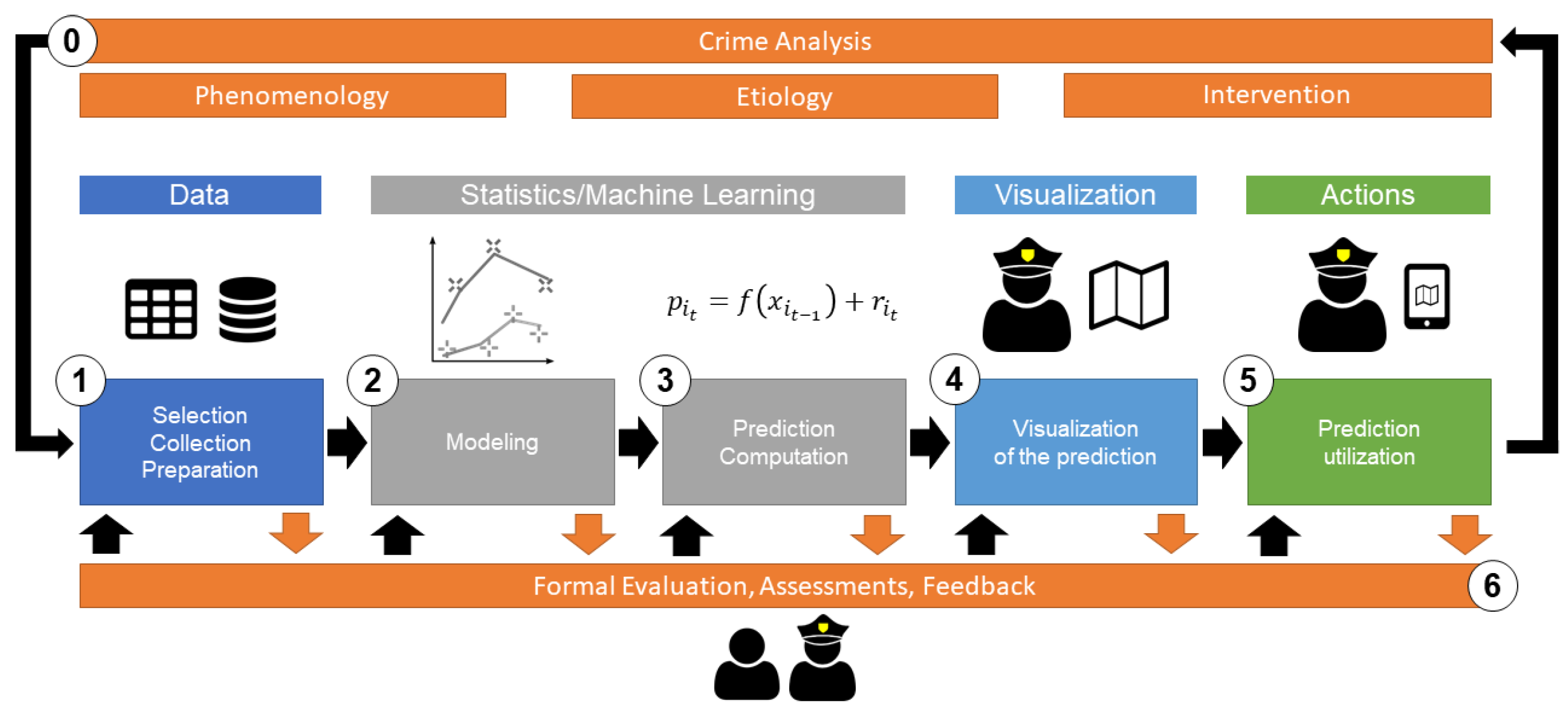
The classical crime forecasting approach in the SKALA project focuses on using predictive policing as a method to compute spatial crime risks. In practice, predictive policing involves several steps and processes that build on each other, starting with analyzing the specific offense and the collection and processing of data required for crime prediction. The illustrated methodical process (Figure 1) allows an insight into the individual steps for implementing predictive policing from the police department’s point of view, as it also took place in SKALA. Deviations are conceivable, but at least similar designs are likely to be present whenever machine learning technologies are used.).

All process steps depend on the available data, the data acquisition, and the preparation of the data for further processing. For predictive policing, data quality is therefore of crucial importance. In this context, data acquisition problems are conceivable, for example, when recording a residential burglary’s suspected and not precisely determinable time. Moreover, data uncertainties can arise on the side of the police forces if crimes are legally misjudged or reported late by the victims, which cannot be ruled out for the crime of residential burglary, for example. In addition, the fundamental problem is that crime phenomena cannot usually be fully described with the available data, especially when unobservable or unquantifiable effects are important. Thus, when making crime forecasts, the question must be asked whether the anticipated crime event occurred independently of the criminological and mathematical models used.

A deliberate decision was made to avoid an exclusively data-driven approach in order to produce crime forecasts, and a theory-driven approach was adopted. Specifically, due to the increasing digital availability of data and the further development in the field of big data processing, data mining approaches—for the prediction of feature characteristics or data points—are also increasingly represented in the methodological discussion on predictive policing [11] (p. 8). Data mining covers (partially) automated methods for analyzing data sets, which can find statistical correlations and provable patterns [12]. Data mining approaches go beyond assumption-driven multivariate data analysis. They can also find non-linear or only partially existing correlations that might have remained undetected during the theoretical derivation of hypotheses from tentatively proven theories. An exclusively data-driven approach must be viewed critically, especially in the context of predictive policing, since plausible assumptions about possible causal relationships already exist for the vast majority of criminal phenomena, which cannot simply be ignored. Likewise, methods of data-driven approaches are subject to the assumption that the input data describe the phenomenon to be analyzed to the degree that automatic pattern and group identification do not occur based on spurious correlations. Especially with regard to data protection, principles such as data economy, and the difficulty of analyzing highly complex phenomena such as crime, it becomes clear that purely data-driven methods should not be used alone in the area of predictive policing. This is based on the fact that crime cannot always be clearly objectified and thus represented within a data set [13].

The theory-driven approach ensured that the used model was based on robust scientific theories and research findings. This distinguished the approach from many other predictive policing methods, which are often based only on the near-repeat approach, which refers to the empirically-proven observation that crime recurs in the same or adjacent locations within a given period [14] (p. 414) [15] (pp. 368 ff.). In practice, the probabilities of residential burglaries, burglaries from commercial properties, and motor vehicle offenses were calculated based on spatial data for residential quarters in selected police districts of NRW.

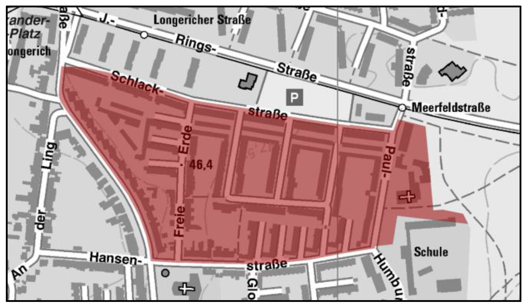
A three-stage procedure was chosen for this purpose. First, spatio-temporal clusters of crime data were calculated based on the near-repeat approach, which refers to a period of 14 days and a radius of 500 m for the residential burglary. The collected crime data mainly included the time and location of the offense, the modus operandi, and the proceeds of the crimes (property stolen). The calculated spatio-temporal clusters were transferred to the residential district level. The residential districts were areas characterized by a number of 400 households per quarter (see Figure 2). For NRW, this resulted in 18,875 residential districts. A uniform size at the household level was chosen because grid cells can lead to over- or underestimation of offenses.

Second, random forest models got a subset of influencing variables out of the socio-economic data. These data were chosen because of their statistical impact on the occurrence of crime. They included information on the residential location, such as population structure, building construction, income, infrastructure connections, and mobility indicators. In this step, random forest models were used to avoid overfitting [16,17]. The advantage of this application is the relatively easy operability and the possibility to perform initial data analysis tasks in a short time, including model and forecast generation. The decision tree models had a comparatively good performance. In addition, they are transparent and comprehensible, so they were favored within this framework. Third, the modeling and forecasting were performed based on the previous results and selected data within a linear regression model.

The areas for which the highest crime probabilities were calculated compared with other areas of the entire forecast area are defined as forecast areas. Their share was limited to about 1.5 percent of the total number of quarters in each police district for practical reasons, such as planning policy measures and allocating and distributing limited police resources.

The calculation of crime probabilities was based on the total area of every single police authority. This procedure ensured that the individual risk of residential burglary for each residential quarter could be determined in the forecast week, as many other predictive policing methods only refer to sub-areas of cities or regions.

The methodological implementation of the model and forecast generation described above focuses primarily on long-term statistical considerations. In the course of SKALA, the pilot authorities repeatedly criticized that future crime series, such as a particular modus operandi, was not reflected in the forecasts. Analyses based on the available series of crimes from the police authorities showed that differentiation from other series or individual crimes was not possible based on the available data material. However, the homogeneity of the characteristics within the respective series was always high. Nevertheless, as a supplement to the statistical and decision tree-based approach of the model and prognosis generation, a second forecast model was developed, which focused on possible series of crimes. This so-called analytical model was independent of the more comprehensive statistical model and supplemented it, depending on the data situation.

3.2. Risk Terrain Modelling

The Risk Terrain Modelling (RTM) approach is a method used to compute the future risk of crime in specific places. Unlike other methods such as hotspot mapping, the calculations with RTM are not, or rather not only, based on crime data but also include geographical characteristics of places [6] (p. 50). RTM is a classification approach that characterizes an area’s risk for crime based on its environmental characteristics [6] (p. 51). Therefore, new hotspots are predicted based on their similarities to other ‘known’ hotspots. The result might be a map of places that did not see any crime but should be considered risky places because of their similar spatial risks compared to crime hotspots. The spatial risk profiles generated are derived from the respective geographic characteristics of the space, which can be identified as risk factors for crime. Studies suggest that the prediction accuracy of the RTM models is better than that of classic hotspot models [18]. However, the correlations found in such models do not necessarily imply a meaningful and substantively justifiable causality. They are usually the results of the “unsupervised learning” method, intended to identify previously unknown correlations or patterns without categorizing the data [19].

In SKALA, the RTM instrument should primarily be made available to police forces with a deficient number of cases in relation to their area (rural regions), as this makes it difficult to use the previously described crime forecasting model, which particularly results from the fact that the models are primarily based on patterns of crime events that are close in time and space. Therefore, alternative model approaches were sought that are more strongly based on the influence and distribution of socio-economic, building-specific, and infrastructural attributes and their distribution in space.

In the classical RTM, risk factors are determined from a large number of space-specific attributes using statistical methods, which significantly influence the risk burden (number of events per unit of space and time) for a selected offense. The mathematical model underlying the relationship between the significant characteristics and the risk burden enables a forecast calculation of the expected risk of crime. Following this, a risk map can be generated for the entire space of a selected authority. The temporal validity of such a map is strictly linked to changes in the area-specific characteristics and the number of cases, which in rural regions are subject to relatively minor changes on short time scales.

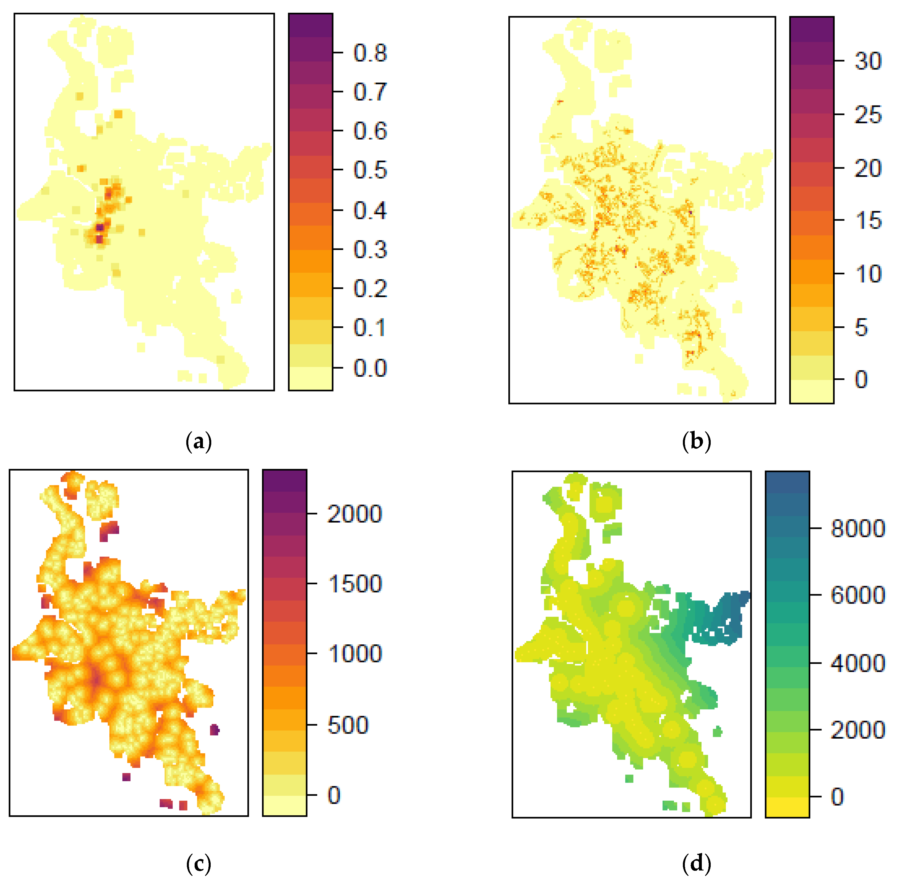
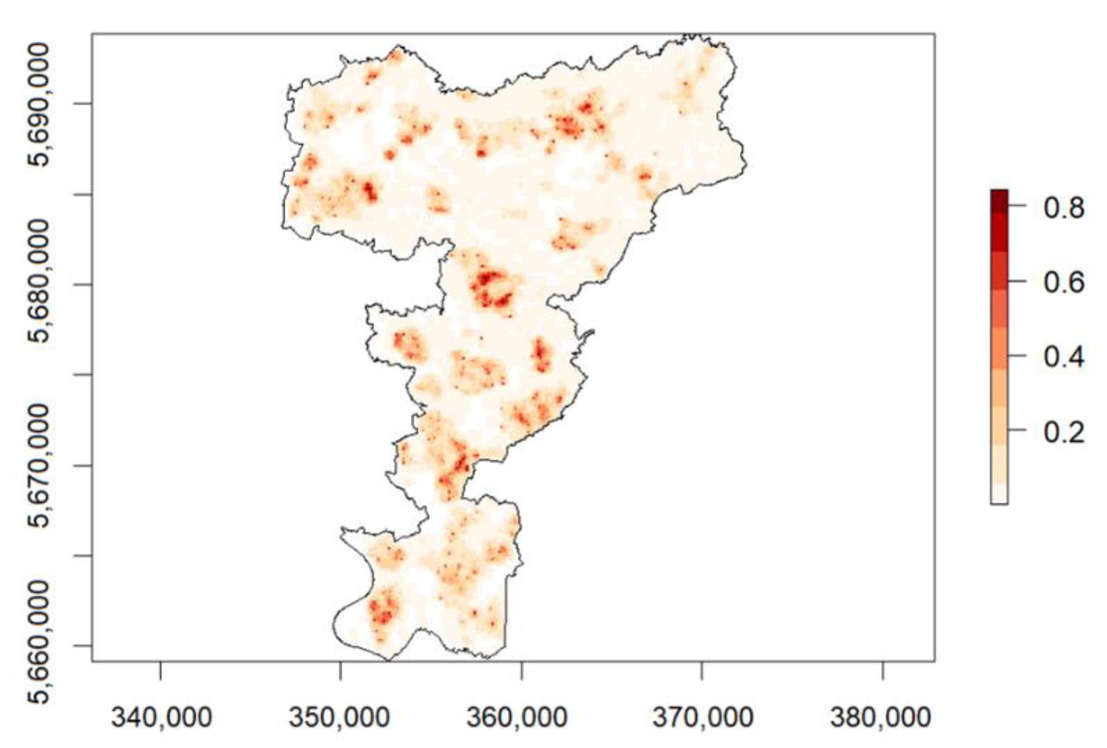
The existing socio-economic and other freely available data, such as point data of bus stops, banks, and supermarkets, were processed, calculated, and aggregated for a uniform grid of 100 × 100 m to test the RTM approach. Figure 3 shows example density maps of different variables for the same city. In the classic RTM approach, the individual input variables are processed in binary form for each raster cell. This means that for each variable and raster cell, it is determined whether the variable is present in the raster cell or not. In the course of development, it quickly became apparent that this approach was insufficient to provide satisfactory results. Therefore, a modified approach was used to convert the existing variables to density-based units, allowing better differentiation of the individual variables’ spatial distribution. Another deviation from the classical RTM is the inclusion of variables calculated from the characteristics of the historical processes, such as the average distance of residential burglary to the three nearest residential burglaries (relative to the center of each grid cell).

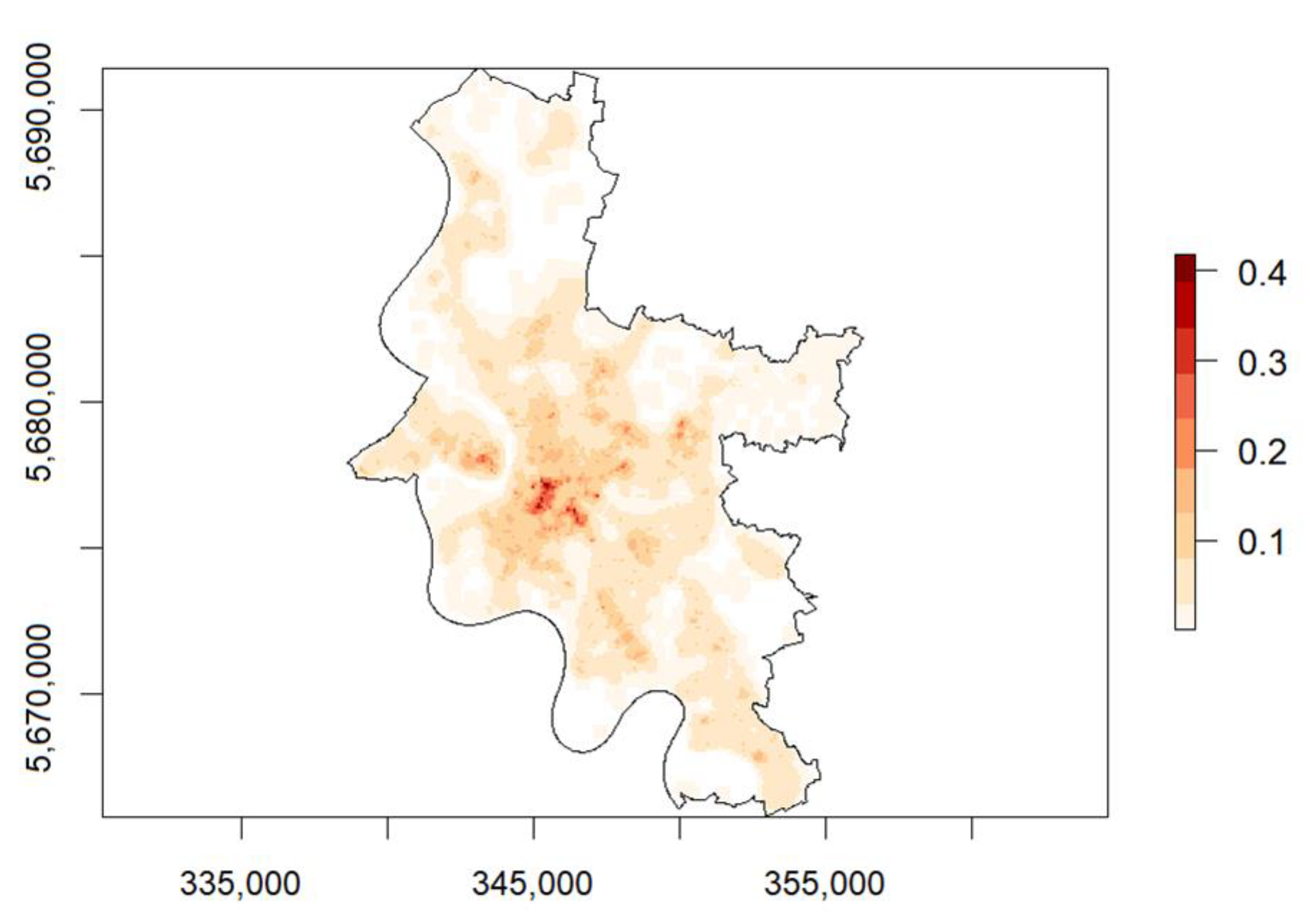
The result for a risk map depends significantly on the assumed relationship between the target variable and the input variables. The different model algorithms realize the mathematical formulation of this problem. The classical RTM formulation is based on Poisson regression. Figure 4 shows an example of a risk map based on Poisson regression. Alternatively, the risk determination can be conceived as a classification problem using common methods such as RF (random forest) or SVM (support vector machine). The main difference between the two formulations in a risk map is the interpretation of the risk load. While a Poisson regression gives a non-scalable risk number for a grid cell that is only valid for the respective authority (for example, a grid cell with a risk number of 5.7 in one city would have a different meaning than a grid cell with the same risk number in another city), the classification gives a probability for the occurrence of an event for each grid cell similar to the previous forecast model used in SKALA (see Figure 5).

As quality criteria for the comparison of the different models, the quality measure of deviance was chosen for the Poisson regression. Deviance indicates how well the significant variables and model parameters determined in the model can describe or reproduce the original statistical distribution of the target variable. For the RF and SVM classification models, the quality measures AUC and PrecRec were chosen. For the AUC value, the closer the AUC value is to 1, the better the model prediction. An AUC value of 0.5 would mean that the model does not predict better than chance. A maximum AUC value of 1 means that all areas were predicted exactly correctly. PrecRec stands for the sum of the quality measures Precision and Recall.

3.3. Time Series Analysis

Time series analysis offers the possibility to detect patterns in the temporal change of crime data, which play a major role, especially in crime prediction and prevention. Methods such as time series decomposition and autoregressive integrated moving average (ARIMA) modeling can be used for this purpose. A decomposed crime time series consists of the original time series and the three decomposed parts with the estimated trend component, seasonal component, and remainder component. The calculation of trends and seasonality are used for the long-term prediction of crime events to facilitate strategic planning in police agencies [20,21]. Several studies, e.g., Malik et al. [22] and Borges et al. [23], use STL as an initial time series analysis for later modeling a predictive policing approach. Furthermore, this approach allows statements about recurring and changing temporal components of crime without considering socioeconomic or demographical information.

ARIMA modeling is a powerful tool for time series analysis and short-term forecasting. Since ARIMA was successfully applied for predictions in economics, marketing, industry production, and social problems, it was also applied for forecasting property crime [20]. In this study, the ARIMA model was used to predict one week in advance from the observations on property crime, but only for the whole city and not for districts. ARIMA has the potential to enable crime prediction by only using offense data, as well as analyzing temporal crime patterns on different spatial scales by spatial data aggregation [24]. In crime research and strategic planning in police work, information on possible future events in crime data enables short- and long-term orientation and the recognition of changes and recurring patterns.

For time series analysis, a raw time-series signal was constructed out of the criminal records for each analyzed offense, e.g., residential burglary, over a period of five years from 1 January 2017 to 31 December 2021. The number of cases per offense per time unit was aggregated for a sub-region. Thus, only the time and location information of the offense were used. Weekly aggregated offense data on residential district and city level were considered for the time series analysis. Analyses based on daily data were considered problematic due to the small offense numbers.

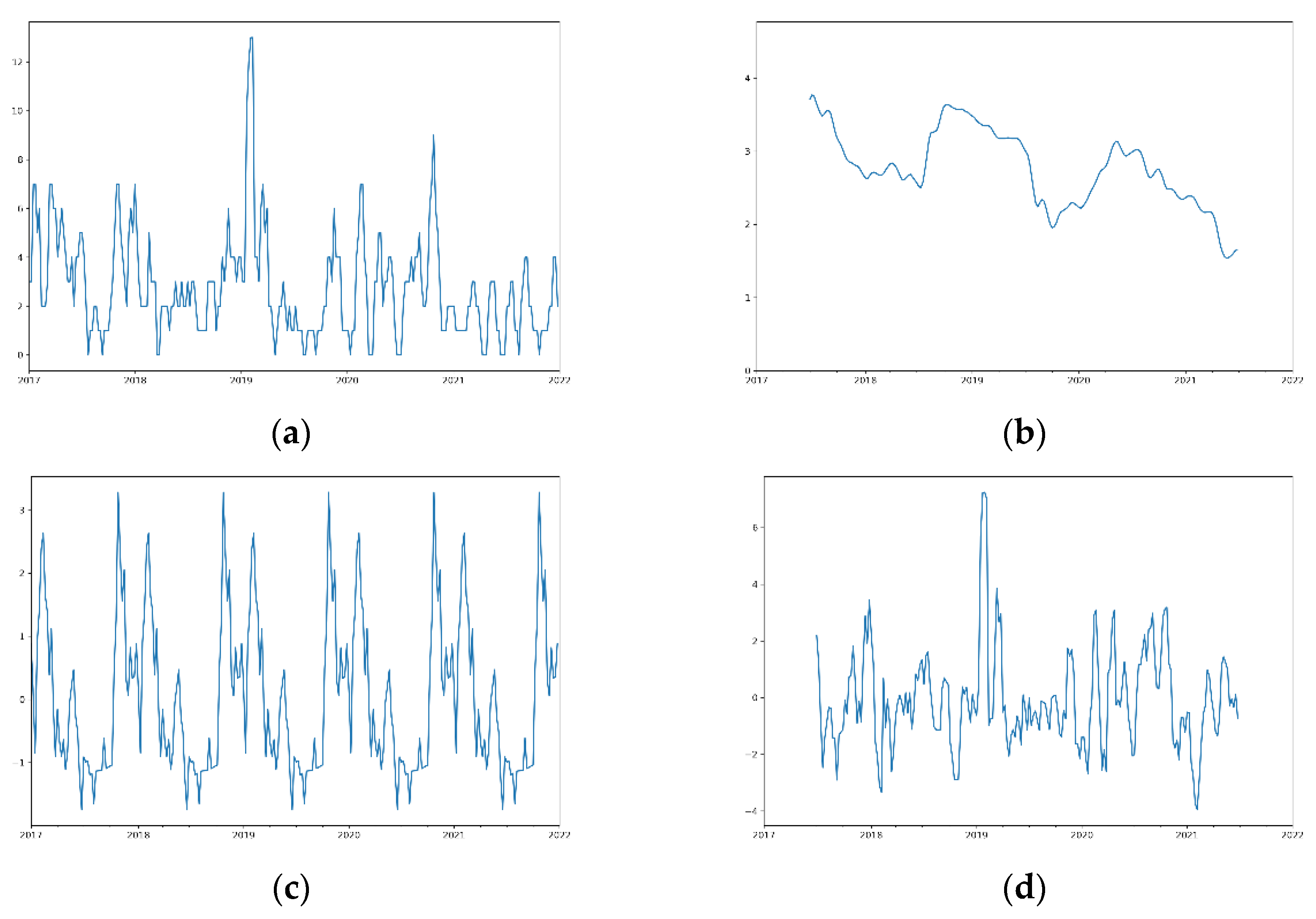
In the first step, a time series decomposition was performed on daily aggregated offense data. The Seasonal Time Series Decomposition based on Loess (STL) is a filtering method for separating three components from a seasonal time series, namely trend (T), season (S), and the remainder (R) [25]. The first component, the trend at the time, indicates the series’ long-term increase or decrease. The second component, the seasonality, indicates whether the time series is modified by seasonal influences, referring to one cycle per year in this case. The third component, the remainder, represents any residual noise in the data. Since STL is an additive model, the time series (Y) at the time (t) can be described as follows [23]:

$$Y_T=T_t+S_t+R_t$$

(1)

The output of this process is the separation of the original time series of criminal record entries into two distinct derivatives: the trend and the season.

Daily aggregated offense data on residential districts were used for time series decomposition.

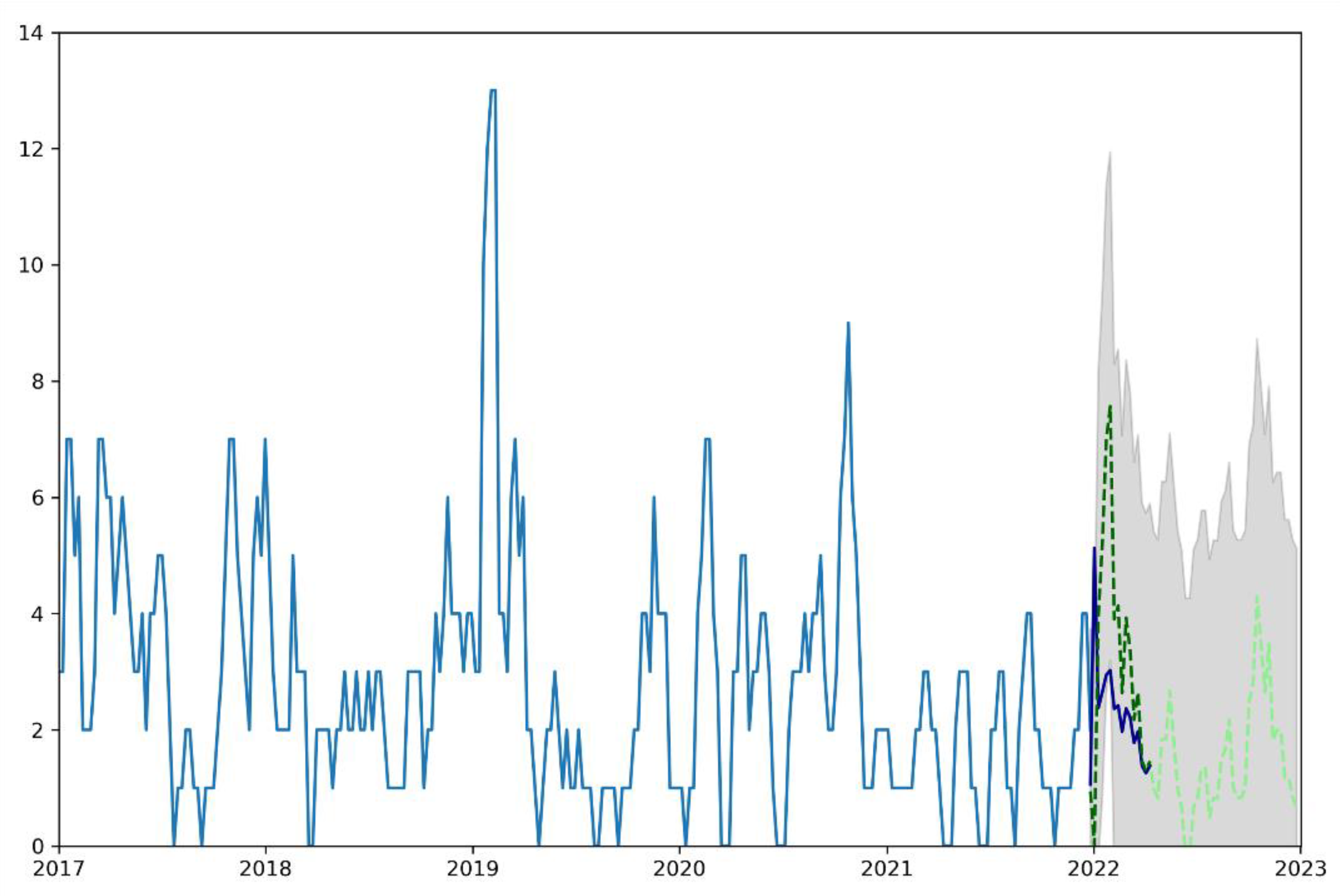
Time series analysis can also be utilized in the process of prediction. In a second step, the autoregressive integrated moving average (ARIMA) model introduced by Box and Jenkins [26] was used to forecast the number of crime events for periods of one week and one month. This model can provide accurate forecasts over relatively short periods [20].

The autoregressive (AR) models attribute current observations only to past observations. In moving average (MA) processes, however, observations are attributed not only to the observations but also to the non-observed error of the past periods, which also influences future observations. Thus, ARIMA models take advantage not only of the observed past observations but also of information that is not described directly in the time series but is defined as the error of the prediction. ARIMA models combine AR models and MA processes as follows:

$$y_t=\alpha +{\varnothing }_{1y_{dt-1}}+{\varnothing }_{p{y}_{dt-p}}+{\theta }_{1{\epsilon }_{t-1}}+{\theta }_{q{\epsilon }_{t-1}}+{\epsilon }_{\tau }$$

(2)

Here, y_d is the d-fold differentiated observations that can follow an AR process with p orders and an MA process with q orders. Therefore, the task is to specify the parameters d, i.e., the order of the necessary integration or differentiation, as well as p and q in the ARIMA (p, d, and q) model [20,27].

The ARIMA model was applied for weekly aggregated offense data at the residential district and city levels.

4. Results and Discussion

4.1. Crime Forecasting

By testing predictive policing as a theory-based approach, the primary purpose of this study was to support strategic and target-oriented police work that identified potential hotspots at an early stage based on known crime-relevant factors. The aim was to achieve a resource-efficient deployment of police forces and, ideally, reduce the frequency of crime. The results show that it is often possible to calculate higher crime probabilities in the chosen spatial reference for residential burglaries, commercial burglaries, and motor vehicle offenses compared with the basic statistical probabilities. Depending on the modeling, the probabilities of residential burglaries in selected residential districts were, on average, about ten times higher than those of a random area selection. Nevertheless, it was found that the compilation of weekly crime forecasts in more rural districts was ineffective due to a relatively low number of cases. However, analyses focusing on the structural differences between urban and rural regions have found approaches that make it possible to determine the probability of burglary in more rural regions so that it was possible to compute crime forecasts for the entire state.

In addition, the influence of the socio-structural data on residential burglaries was also examined. In summary, the results show that the influencing strengths of the variables varied greatly depending on the season and district. Accordingly, the results are not automatically transferable to other districts or periods. Furthermore, it was shown in this context that the model quality crucially depended on the quality and temporal availability of the data.

4.2. Risk Terrain Modelling

In both cases, modifying the classical RTM approach to classification and Poisson models led to significantly better model performance. For example, a Poisson model showed a model improvement of about 35 to 40 percent. Deviance with dynamic variables (calculated based on historical police data) was significantly lower than deviance with purely static variables like sociostructural data. Conversely, this finding means that a RTM map created with only static variables is less reliable in its informative value than a RTM map with dynamic and static variables. The quality of the dynamic variables, on the other hand, decreases with decreasing density of the number of cases, i.e., with progression from urban to rural regions.

In addition, the analyses showed that the weighting of the variables among each other is an important aspect of variable selection. The rough distribution of weights between two different model approaches is largely similar. For example, the dynamic variables are often in the upper weight range. The analyses have also shown that both the weighting of the variables among each other and the selection of the variables themselves can be subject to strong local variations. Depending on the selected period, both model approaches enable a statement to be made for the same temporal scope in each case. For example, a model that has been trained with historical data from the last six months enables a forecast for the following six months. Due to the very slowly changing socio-structural data and strongly fluctuating local dynamic variables, there is a compelling lower temporal horizon limit for which a RTM map can be generated reliably. However, no universally valid lower boundary can be defined due to the strong local fluctuations.

In summary, it can be shown that a spatial risk assessment is also possible for more rural police departments in NRW. Due to the high computation times of the model for the large spaces and the desire for a fine-scale grid, a seasonal risk assessment is necessary to support strategical decision-making processes in the police authorities.

4.3. Time Series Analysis

The results of the time series decomposition of the weekly aggregated offense data on the residential district level for NRW are presented in Figure 6, exemplarily for residential burglary. The estimated trend component revealed a decrease in residential district level residential burglaries from 2017 until December 2021. Regarding the seasonal component, an increase in the winter terms was detected, and a decrease in the summer terms throughout the entire analysis period was also detected. These temporal and spatial patterns can be applied to metropolitan cities. The procedure cannot be transferred to more rural regions due to the small number of cases.

The results can likewise be transferred to all residential districts. In general, areas close to the city center, which are densely populated, show similar temporal patterns, as shown in Figure 6. The procedure cannot be transferred to peri-urban areas, which tend to be characterized by a lower population density and thus have lower offense numbers. In these areas, approaches such as integrating the spatio-temporal clusters or residential district aggregation can help make valid calculations.

The experimental results produced for the cities and residential districts in NRW using an ARIMA model of the weekly aggregated offense time series support the value of crime time series analysis. The results for residential burglary are shown exemplarily for a selected residential district in Dusseldorf in Figure 7. The fitting of the ARIMA model shows that both seasonal components and the initially increasing and subsequently decreasing trend could be captured. The higher case numbers in the winter months could also be mapped. The prediction of offense numbers for the following 16 weeks and one year show that both the decreasing trend and the seasonal component are included. The offense numbers recorded by the police fall within the confidence intervals of the predicted values. Thus, this method is promising, for example, for the prediction of residential burglaries and long-term planning and strategic orientation of the police authorities. The ARIMA model is a way to look at both long-term changes and seasonal components of crime. The use of the model is advantageous for crime data, as studies have shown that ARIMA works better than complex Artificial New Networks, for example, in the case of a small number of datasets [28]. The fitted ARIMA model can forecast future points in a series [20].

In general, time series analysis is a helpful approach to analyzing seasonal and long-term patterns of offense numbers. The conclusions can be drawn from these results for the following weeks or months as to what extent offense numbers are likely to increase, decrease, or remain constant. Therefore, long-term strategic decision-making processes in the police authorities can be supported.

5. Potential and Limitations

Spatio-temporally-based statistical techniques offer police agencies the potential to optimize their operational and strategic planning based on predictions and to take necessary action before a crime occurs. Targeted control of the forces or the alignment of operational focal points in specific crime areas is possible. Changes in crime can be detected earlier based on such calculations.

In evaluating crime forecasting methods, data quality is crucial concerning data uncertainty. Data uncertainty refers to the problem that it is usually unknown as to what extent errors are contained in the collected and utilized data. In this context, data collection problems such as measurement uncertainties are conceivable, e.g., when re-cording the suspected time of a burglary. For data collection in the context of police forces, a source of uncertainty is the fact that criminal offenses are either legally misjudged or are reported late by the victims, which is not uncommon for the criminal charges of burglaries [8]. In addition, the data quality of the data collected in the field of policing is often low, as periods and localities are not (or cannot) always be precisely defined. Similarly, it is challenging to predict offenses that should be prevented by increased police presence. There is often a lack of knowledge about whether police presence has prevented offenses or whether the predictive models are outputting inaccurate risk estimates.

Overall, crime forecasting methods offer a wide range of possible applications that enable criminal expertise to be enriched by scientific findings.

References

1. Seidensticker, K.; Bode, F. Good policing in times of abstract police. In The Abstract Police; Terpstra, J., Salet, R., Fyfe, N., Eds.; Eleven International Publishing: Den Haag, The Netherlands, 2022; pp. 169–182. [Google Scholar]
2. Fotheringham, A.S.; Brunsdon, C.; Charlton, M. Geographically Weighted Regression. The Analysis of Spatially Varying Relationships; John Wiley & Sons Ltd.: West Sussex, UK, 2002. [Google Scholar]
3. Ratcliffe, J. Crime mapping: Spatial and temporal challenges. In Handbook of Quantitative Criminology; Piquero, A.R., Weisburd, D., Eds.; Springer: New York, NY, USA, 2010; pp. 5–24. [Google Scholar]
4. Bundeskriminalamt (BKA). PKS Jahrbuch 2018, Band 4, Version 3.0; BKA: Wiesbaden, Germany, 2019. [Google Scholar]
5. Seidensticker, K. SKALA—Predictive Policing in North Rhine-Westphalia. Eur. Law Enforc. Res. Bull. 2021, 21, 47–60. [Google Scholar]
6. Perry, W.; McInnis, B.; Price, C.; Smith, S.; Hollywood, J. Predictive Policing. The Role of Crime Forecasting in Law Enforcement Operations; RAND Corporation: Santa Monica, CA, USA, 2013. [Google Scholar]
7. Pearsall, B. Predictive Policing: The future of law enforcement. Natl. Inst. Justice J. 2010, 266, 16–19. [Google Scholar]
8. Seidensticker, K.; Bode, F.; Stoffel, F. Predictive Policing in Germany. Konstanzer Online-Publikationssystem (KOPS). 2018. Available online: http://nbn-resolving.de/urn:nbn:de:bsz:352-2-14sbvox1ik0z06 (accessed on 5 July 2022).
9. Landeskriminalamt Nordrhein-Westfalen (LKA NRW). Abschlussbericht Projekt SKALA; LKA NRW: Düsseldorf, Germany, 2018. [Google Scholar]
10. Bode, F.; Stoffel, F.; Keim, D. Variabilität und Validität von Qualitätsmetriken im Bereich von Predictive Policing; KOPS: Konstanz, Germany, 2017. [Google Scholar]
11. Pollich, D.; Bode, F. Predictive Policing: Zur Notwendigkeit eines (sozial)wissenschaftlich basierten Vorgehens. Poliz. Wiss. 2017, 3, 2–12. [Google Scholar]
12. Fayyad, U.; Piatetsky-Shapiro, G.; Smyth, P. The KDD Process for Extracting Useful Knowledge from Volumes of Data. Commun. ACM 1996, 39, 27–34. [Google Scholar] [CrossRef]
13. Seidensticker, K. Predictive Policing—Herausfordernde Polizeiarbeit der Zukunft? In Zukunft Digitaler Polizeiarbeit; Rüdiger, T., Ed.; Verlag für Polizeiwissenschaft: Frankfurt am Main, Germany, 2021; pp. 41–76. [Google Scholar]
14. Bernasco, W. Them Again? Same-Offender Involvement in Repeat and Near Repeat Burglaries. Eur. J. Criminol. 2008, 5, 411–431. [Google Scholar] [CrossRef] [Green Version]
15. Gluba, A.; Heitmann, S.; Hermes, N. Reviktimisierung bei Wohnungseinbrüchen. Eine empirische Untersuchung zur Bedeutung des Phänomens der (Near) Repeat Victimisation im Landkreis Harburg. Kriminalistik 2015, 6, 368–375. [Google Scholar]
16. Barnard, D.; Germino, M.; Pilliod, D.; Arkle, R.; Applestein, C.; Davidson, B.; Fisk, M. Cannot see the random forest for the decision trees: Selecting predictive models for restoration ecology. Restor. Ecol. 2019, 27, 1–11. [Google Scholar] [CrossRef]
17. Bellman, R. A Markovian decision process. J. Math. Mech. 1957, 6, 679–684. [Google Scholar] [CrossRef]
18. Wang, X.; Brown, D. The spatio-temporal modeling for criminal incidents. Secur. Inform. 2012, 1, 1. [Google Scholar] [CrossRef] [Green Version]
19. Hastie, T.; Tibshirani, R.; Friedman, J. The Elements of Statistical Learning. Data Mining, Inference, and Prediction, 2nd ed.; Springer: Berlin/Heidelberg, Germany, 2009. [Google Scholar]
20. Chen, P.; Yuan, H.; Shu, X. Forecasting crime using the arima model. In Proceedings of the 5th International Conference on Fuzzy Systems and Knowledge Discovery, Shandong, China, 18–20 October 2008; IEEE: Piscataway Township, NJ, USA, 2008; pp. 627–630. [Google Scholar]
21. Islam, K.; Raza, A. Forecasting crime using ARIMA model. arXiv 2020, arXiv:2003.08006. [Google Scholar]
22. Malik, A.; Maciejewski, R.; Towers, S.; McCullough, S.; Ebert, D.S. Proactive spatiotemporal resource allocation and predictive visual analytics for community policing and law enforcement. IEEE Trans. Vis. Comput. Graph. 2014, 20, 1863–1872. [Google Scholar] [CrossRef] [Green Version]
23. Borges, J.; Ziehr, D.; Beigl, M.; Cacho, N.; Martins, A.; Araujo, A.; Bezerra, L.; Geisler, S. Time-series features for predictive policing. In Proceedings of the IEEE International Smart Cities Conference (ISC2), Kansas City, MO, USA, 16–19 September 2018; IEEE: Piscataway Township, NJ, USA, 2018; pp. 1–8. [Google Scholar]
24. Roy, S.; Bhunia, G.S.; Shit, P.K. Spatial prediction of COVID-19 epidemic using ARIMA techniques in India. Model. Earth Syst. Environ. 2021, 7, 1385–1391. [Google Scholar] [CrossRef] [PubMed]
25. Cleveland, R.B.; Cleveland, W.S.; McRae, J.E.; Terpenning, I. STL: A seasonal-trend decomposition procedure based on loess. J. Off. Stat. 1990, 6, 3–73. [Google Scholar]
26. Box, G.E.; Jenkins, G. Time Series Analysis: Forecasting and Control; Holdan-Day: San Francisco, CA, USA, 1970. [Google Scholar]
27. Tariq, H.; Hanif, M.K.; Sarwar, M.U.; Bari, S.; Sarfraz, M.S.; Oskouei, R.J. Employing Deep Learning and Time Series Analysis to Tackle the Accuracy and Robustness of the Forecasting Problem. Secur. Commun. Netw. 2021, 2021, 5587511. [Google Scholar] [CrossRef]
28. Jha, S.; Yang, E.; Almagrabi, A.O.; Bashir, A.K.; Joshi, G.P. Comparative analysis of time series model and machine testing systems for crime forecasting. Neural. Comput. Appl. 2021, 33, 10621–10636. [Google Scholar] [CrossRef]
Figure 1. The predictive policing process. Adapted with permission from Ref. [10]. 2017, Bode/Stoffel/Keim.
Engproc 18 00039 g001
Figure 2. Example of a residential district. Reprinted with permission from Ref. [9]. 2018, LKA NRW.
Engproc 18 00039 g002
Figure 3. Input variables using the example of Düsseldorf with the (a) variability of parking lots, (b) street light density, (c) car density, and (d) minimum distance to train stops taken from Open Street Map (OSM).
Engproc 18 00039 g003
Figure 4. RTM (Poisson model) for 100 × 100 m grid cells in risk classes over six main percentiles for the police authority Düsseldorf.
Engproc 18 00039 g004
Figure 5. RTM (classification model) of the police authority Mettmann.
Engproc 18 00039 g005
Figure 6. Time series decomposition of residential burglary in one exemplary residential district in Dusseldorf from 2017 to 2021 with (a) raw time series, (b) trend, (c) season, and (d) remainder.
Engproc 18 00039 g006
Figure 7. Time series of residential burglary events in a residential district in Dusseldorf with the ARIMA-modelled prediction for the first 16 weeks (dashed dark-green line) and 52 weeks (dashed light-green line) in 2023.
Engproc 18 00039 g007
Publisher’s Note: MDPI stays neutral with regard to jurisdictional claims in published maps and institutional affiliations.