1. Introduction
The use of chemical agents in agriculture is a necessary practice to maintain high production levels. However, the role of policies (e.g., the European Common Agricultural Policy—CAP [
1], pesticides, and water quality directives) is to foster the reduction in chemicals in the agricultural production process to maintain the biodiversity and to reduce the environmental impacts. At the same time, there is the need to collect suitable data on the agricultural inputs and to monitor the effects on the environment (soil and water). Monitoring is also a steppingstone to assess the performance and results of the policies in the agri-environmental domain.
The monitoring process should not stop at the surveying step, it needs to follow a more complex analysis to identify the origin and destination of the chemical substances in the environment. Similar works have been conducted in the Netherlands, where an atlas for surface water was created for analyzing the concentration level of pesticides, their evolution over time and how they can be linked to land uses [
2]; in Spain, the dispersion behavior of pesticides was studied along the water basin of the Júcar river [
3].
The aim of this work is to understand the relationships between specific chemicals traced in surface water and the typology of land use located around the water monitoring stations. We propose a methodology for the production of a land use map with a very high geometric, thematic, and temporal resolution, especially for the agricultural land use. We use geospatial administrative data from European agricultural paying agencies to produce an improved land-use map compared to the ordinary land cover/use map available at national/European level (e.g., Corine Land Cover [
4]). The methodology is complemented by the integration of the land-use map with the georeferenced water quality measures and a sound statistical analysis.
2. Materials and Methods
This work uses the geo-referenced data from the Italian Paying Agency (AGEA), the body managing the CAP agricultural subsidies, and from the Italian Institute for Environmental Protection and Research (ISPRA). Three land-use vector layers, from AGEA, with polygon geometry were acquired and processed: Land Parcel Identification System—LPIS (2016) [
5]; Geo-spatial Aid Application—GSAA (2018); Gis Soil (2018).
One vector layer with point geometry containing the georeferenced surface water monitoring stations with the associated database was acquired from ISPRA (2016) [
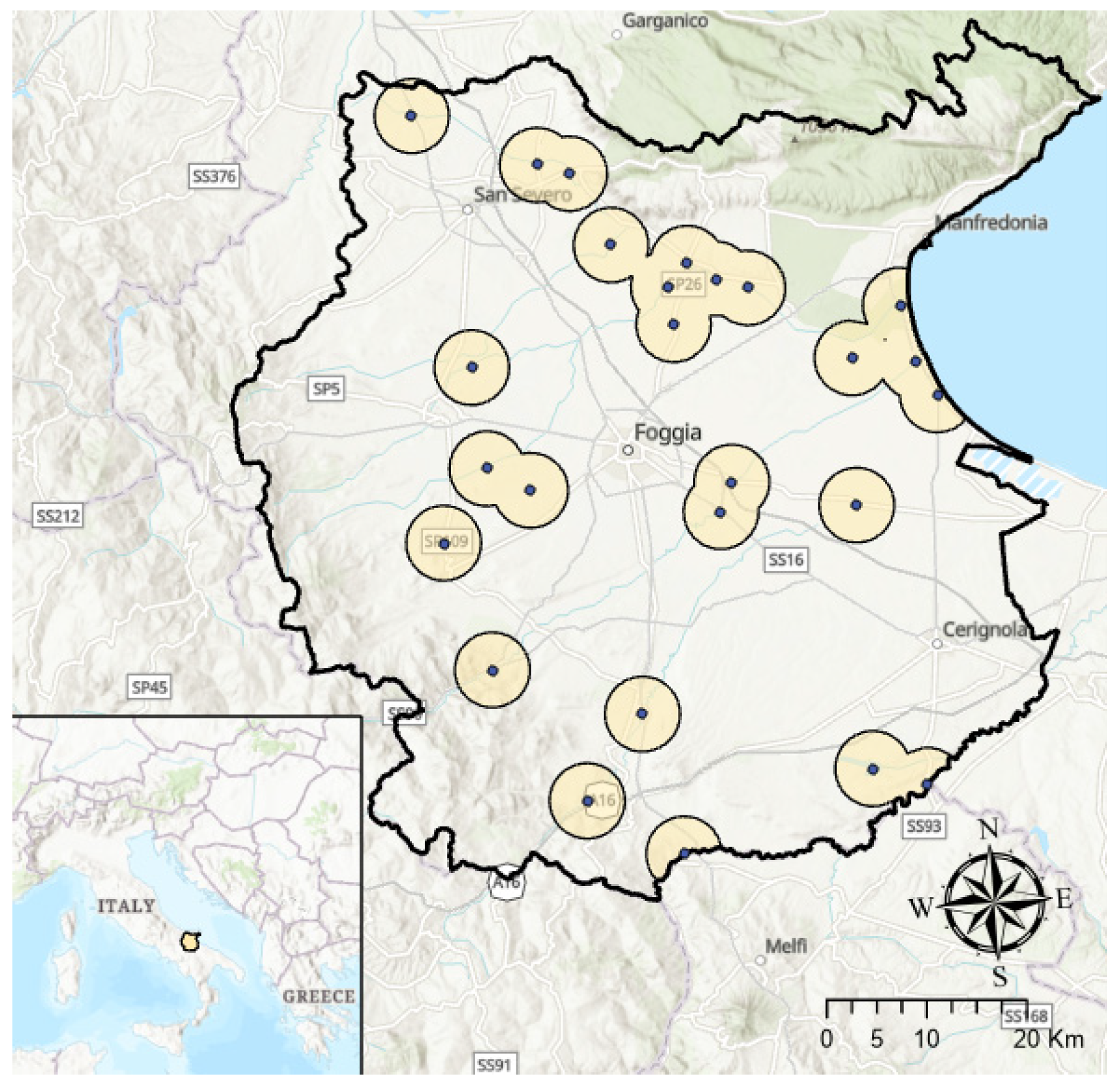
6]. All the vector layers were converted to the common geographic reference system WSG 84/32N. The area of interest is a large water basin located in the Foggia Province (Apulia region), South of Italy (
Figure 1).
2.1. LPIS
The layer is the land-use/cover map created through photointerpretation of very-high resolution imagery (20 cm) carried out with a three-year cycle to cover the whole Italian territory [
5]. The data is structured in polygons associated with information such as a numerical identifier and a generic type of land use/cover (e.g., arable land, permanent crops, forests, urban areas). In some cases, the polygons are classified with detailed land-use codes (e.g., vine instead of permanent crop) through the integration of the photo-interpreted information with ancillary data such as farms’ data and field checks.
2.2. Geo-Spatial Aid Application (GSAA)
The GSAA vector layer includes only the agricultural areas digitized annually by the Italian farms during the administrative procedures for requesting the CAP agricultural subsidies. The thematic resolution of the layer is very high since it reports, for each cultivated parcel, the crops (wheat, vines, etc.), the intended use (forage, industry, etc.) and quality.
2.3. GIS Soil
The layer can be described as an “intersection” of the layer of the cadastral parcels with the LPIS. GIS Soil is constantly updated by AGEA using its own administrative procedures, such as objective checks on land-use declarations or reviews provided by farms.
2.4. Water Monitoring Stations
The dataset contains the location of the surface water monitoring stations for the period 2015–2016 and the relative tables with the typology and average amount of chemicals. In the study area, there are 26 survey stations unevenly distributed with some clustering in specific areas.
Among the chemical substances traced, we analyzed the presence of isoproturon (CAS 34123-59-6) [
7], a plant protection product used as herbicide in agriculture.
2.5. Integration of the Three Land-Use Vector Layers: The Hybrid Layer
We performed the integration of the three land-use layers to generate a very high-resolution map with an improved geometric, thematic, and temporal resolution compared to the original layers. Before performing the spatial intersection of the vector layers, harmonization of the spatial reference system and geometric and topological check were applied to the original datasets. This process was very challenging due to the nature of the single layers that were produced at different stages of the administrative process, by different actors and with different standards, procedures, and quality controls.
After the pre-processing phase, the three layers were intersected in this order: LPIS-Gis Soil-GSAA. It should be noted that the areas not covered by GIS Soil are mostly roads, city buildings and natural areas that are quite stable during the years. The last step in the generation process is a check on the combination of the two different land-use codes to resolve possible conflicts.
The result is a new hybrid layer with the highest possible thematic and spatial resolution due to the specificity of the GSAA code system.
2.6. Assigning Concentration Values to the Hybrid Layer
The frequencies for the levels of concentration of isoproturon 0.05, 0.1, 0.15, 0.17, 0.2 in the 26 monitoring stations are 1, 1, 3, 1 and 20, respectively.
To extend the observed values to the surrounding area, a buffer of 5 km was created around each survey station [
3]. The underlying assumptions are that the concentration levels are homogeneous in each circle and the observed values are due to the land use within the buffer. The polygons intersecting buffer areas were selected, rasterized, and assigned the respective concentration level.
The resulting land uses were aggregated from 735 classes to 630, and after adding a minimum of 50,000 observations per land use, a total of 12,960,454 points were kept (over the initial 15,772,668, 82.1%) for 21 land uses.
The concentration can assume six values that do not seem to be originated from a continuous space but are more likely to be rounded. For this reason, they are considered as an ordered categorical variable and not a continuous one.
3. Results and Discussion
The results from the elaboration process were put in a 21 × 6 table analyzed through a correspondence analysis [
8,
9] in R software [
10] with the ‘ca’ package. The value of the chi-square statistic is 12,77,406 with 100 degrees of freedom and
p-value = 0; therefore, it is safe to assume some degree of association between these two categorical variables. The total inertia, computed as φ
2 = χ
2/N, which describes the variation in the contingency table is: 0.098.
In
Table 1, the level of inertia associated with each dimension is reported. The use of the first two dimensions explains 71.2% of inertia; adding the third and fourth dimensions would amount to 93.9%, but it would complicate the analysis too much. For this reason, only the first two dimensions were considered.
Table 2 is an extract of the summary for the Rows (land use) while
Table 3 is the summary for the columns (concentration of isoproturon):
Starting the analysis for the rows (
Table 2), we observe that the coordinates for many land uses are clustered in the origin of the axes; therefore, they are close to the average profile. The quality parameter shows that large lakes and water basins, Beans EFA (Ecological Focus Area), polyphite pastures and unspecified tree crops are well represented. Considering now the EFA-type areas, we have three couples of land uses with this specification. While some have low quality levels, their pairs are spaced apart. This shows that the establishment of this type of area could lead to a change in the use of plant protection products (isoproturon).
An unusual behavior can be observed for large lakes and water basins, since it is the furthest from all points and the best represented. It is also associated with the highest inertia. This distance confirms the hypothesis that large water basins have a different behavior than other land uses regarding the concentration of isoproturon (and probably other chemicals).
As regards permanent trees, the behavior of specialized tree cultivations is similar to the behavior of vineyards. On the other hand, olive trees are located more distant and closer to the origin of the axes.
Considering the columns in
Table 3, we observe that the points are distant from each other and do not present a specific pattern. The quality levels are different; the higher concentrations are better represented (probably given the greater sample size) as opposed to the lower ones. It is noted that the highest contraction value is close to the origin of the axes, close to the average profile. In fact, studying the absolute contribution, the level 0.15 contributes the most to the first dimension, while 0.17 does the same for the second.
4. Conclusions
The illustrated approach shows how it is possible to use geo-referenced administrative data and integrate them with environmental datasets for understanding the impacts of the agricultural activities on the environment (water quality). Despite administrative vector layers not being designed for this kind of application, after a process of integration and data preparation, it is possible to obtain a significant improvement in the polygons geometry and in the thematic and temporal resolution. This process can be time consuming and demands a lot of computational power, but it provides a better option to coarse land-use/cover maps available (e.g., Corine Land Cover with a minimum mapping unit of 25 hectares [
4]).
The conducted analysis shows how land uses differ from each other in relation to different concentrations. The used approach is a somewhat simplified approximation of reality, as it can be extended to the entire regional surface and not just to the buffer around the survey station.
The study uncovered methodological and data source limitations that can be addressed in future research. First, it would be advisable to improve the detail of the hydrographic basins. Through the identification of the secondary basins and by considering the terrain slope and the precipitation pattern as additional variables, it would be possible to improve the understanding of the chemical runoff and infiltration processes, also in relation with the farms’ management practices.


