Proceeding Paper

Climate Services for Organic Fruit Production in Valencia Region: Early Frost Forecasting †

1
Data Scientist, GMV Aerospace and Defense S.A., Isaac Newton, 11. P.T.M. Tres Cantos, 28760 Madrid, Spain
2
Project Manager, Spatial Data Analyst, GMV Aerospace and Defense S.A., Santiago Grisolía, 4. P.T.M. Tres Cantos, 28760 Madrid, Spain
*
Author to whom correspondence should be addressed.
Presented at the 1st International Online Conference on Agriculture-Advances in Agricultural Science and Technology, 10–25 February 2022; Available online: https://iocag2022.sciforum.net/.
Chem. Proc. 2022, 10(1), 70; https://doi.org/10.3390/IOCAG2022-12218
Published: 10 February 2022

Abstract

:
The increased occurrence of extreme weather events due to climate change has heightened the need to develop support decision systems that can help farmers to mitigate losses in agriculture. Environmental hazards, such as frost, have a relevant economic impact on crops since they may cause damage and injuries to sensitive crops and, therefore, lead to production losses. The probability of frost occurrences is heavily influenced by local climate conditions. In addition, the extent of damage due to frost also depends on the phenology stages of the crops present in the area of interest. Hence, an early frost warning system at a local scale has the potential to minimize damage to the crops as one can deploy protective mechanisms. In this article, we present models for early forecasting (24 and 48 h) of frost occurrences using stacked machine learning models. We trained the machine-learning models with hourly historical data from a local weather station. The trained model is validated within the timeframe when the crops (organic fruits) are most susceptible to frost for the area of study. We also show the applicability of the model by extrapolating it to a new region. This development is carried out within the framework of the H2020 CYBELE project.

1. Introduction

The increased occurrence of extreme weather events due to climate change has heightened the need to develop support decision systems that can help farmers to mitigate losses in agriculture. Environmental hazards, such as frost, have a relevant economic impact on crops since they may cause several damages and injuries in sensitive crops and, therefore, production losses. Frost is a serious problem for horticultural/fruit-tree production both early and late in the season since the water within the plants and/or fruits may freeze during a frost event. The climate conditions influence the occurrence probability of this kind of event, together with other issues such as vegetation presence, topography and soil type with relevance at a local scale. Passive and active protection methods for frost exist in the market with their different characteristics, effects and costs. Based on the previous affirmation, early warning systems at a local scale with a suitable spatial resolution on frost occurrence and their associated risks are relevant for agriculture. A frost forecast system might help farmers to reduce any possible injuries to their crops since protective methods can be used. In the Valencia region (Spain), the compensations due to extreme weather events amounted to 9 million euros in 2020, and the previsions to 2021 would amount to 4.61 million euros according to the last Agroseguro report [1].
This paper covers the forecasting of frost occurrences using machine learning techniques based on historical data. The Area of Interest (AoI) consists of two different agrarian lands located in Carlet and Belgida municipalities in the Valencia Region. Due to the agricultural practices in the AoIs, farmers usually need 24 to 48 h to prepare frost protection. As a result, this paper focuses on 24 and 48 h forecasting of frost events. Frost forecasting is a challenging problem due to the inherently chaotic nature of local weather patterns as well as the dependency on meteorological and plant physiological factors [2]. Several empirical techniques exist for decision support systems (DSS) with respect to frost forecasting, as reviewed in Ref. [3]. Machine learning approaches are becoming important tools in agriculture DSS with applications in land preparations, crop management, maintenance, plagues control, etc., [4,5]. Such approaches have been used to forecast occurrences of frost with a forecasting window of a few hours [6,7,8,9,10]. On the other hand, this paper attempts to forecast for a much larger forecasting window on the AoI using ensemble learning.

2. Methods

The methods section is divided into the following subsections: In Section 2.1, the definition of frost used in the paper is introduced. It is followed by the characterization of forecasting time and window in Section 2.2. Next, the dataset used in this study and its characteristics are presented. The last section deals with the strategy of creating machine learning-based models.

2.1. Frost Definition

Frost formation occurs when the temperature of a surface becomes lower than 0 °C. The formation of frost can occur due to the incursion of a large-scale cold air mass resulting in the lowering of the temperature below 0 °C. Such an event is known as advective frost and can occur during the day or night. On the other hand, radiation frost is characterized by a clear sky, calm or very little wind, the inversion of temperature and air temperatures that typically drop below 0 °C. Radiation frosts usually occur at night-time. Both kinds of frost generates stress on the agricultural plants and can lead to a potential decrease in yield. To define the condition for the occurrence of frost on agricultural plants, one needs to monitor the temperature of plant surfaces. Such a task is clearly not straightforward to carry out. Alternatively, one can use indirect methods to estimate plant temperature using physiological and thermal properties. As a result, in this article, due to constraints on the type of data available at the agro-climatic stations along with the lack of ground truth, a frost event is defined if the air temperature becomes lower the 0 °C within the forecasting window.

2.2. Forecasting Window and Time
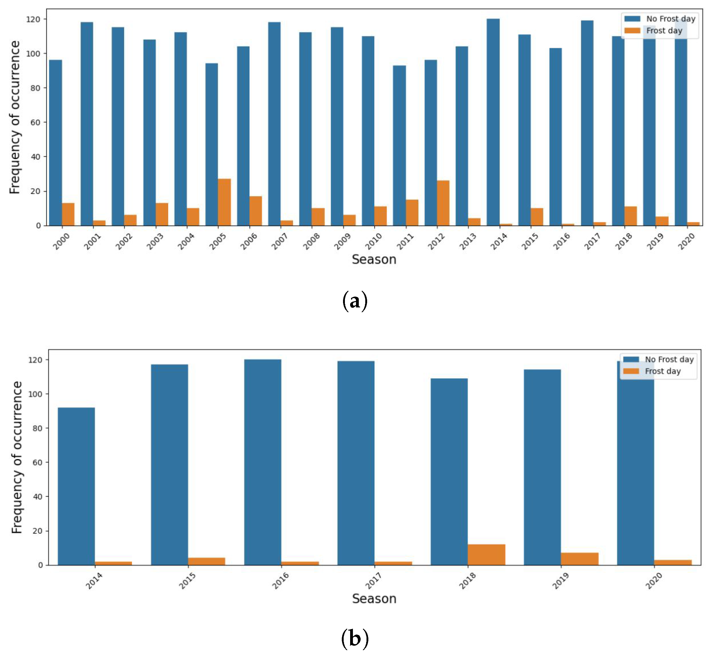
In this paper, frost forecasting will be performed 24 and 48 h ahead. This forecasting window was decided as in the AoI the majority of farmers use anti-frost vitamins such as α-tocopherol and glycerol. As described in Ref. [11], such vitamins have to be applied at least 24–48 h before to have considerable protection. Additionally, in the present AoI, an agricultural cooperative controls the facilities and resources for providing frost protection to individual farmers. To prepare adequately, the cooperative needs around 48 h. Therefore, to give the cooperative time for preparation, the forecasting will be performed each day at noon. Additionally, at Carlet and Belgida, the agronomist in the agricultural cooperative found that from December to March, the organic fruit in that area is most susceptible to frost occurrence. As an example, for peaches (Prunus Persica), delicate phenology stages such as inflorescence emergence and flowering (BBCH code 55–69) happen within this timescale. As a result, we only consider this part of the season for our predictive model.

2.3. Data Sources

The weather data were gathered from two agro-climatic stations near Carlet and Belgida. The agro-climatic station at Carlet is approximately 2–3 km from the agricultural fields, whereas at Belgida, the station is located near the agricultural fields. The Carlet station has hourly climate data from 1999, and the Belgida station has the same from 2013. The agro-climatic station data includes the variables temperature, wind velocity and direction, humidity and precipitation. By defining daily frost events according to Section 2.1, the distribution of frost events at the location of the respective agro-climatic stations is shown in Figure 1. Each season is defined as December to March of the following year. By looking at the distribution of frost events, it is clear that an uncharacteristic amount of temperatures below 0 °C was reached for the seasons in 2005 and 2012. This is taken into account while creating the training and test dataset. As frost events are usually rare, the dataset is highly imbalanced.
Data from the weather stations directly mounted at the agricultural lands at Carlet and Belgida are used as the test dataset for the 2021 season. Such a dataset, though limited in sample size, can provide a hint for the performance and generalized nature of the models developed.

2.4. Machine Learning Models

To create a predictive model, a classification scheme is developed where the target is the presence or absence of a frost event in the 24 and 48 h forecasting window. The strategy is then to employ a type of ensemble machine learning strategy known as blending, which includes the following steps:
(1)
The data from agro-climatic stations are divided into three parts: Training set: Data until 2010 season; Holdout set: Data from the 2010 season up to the 2014 season, and Validation set: Data from the 2010 season up to 2014 season;
(2)
The Test set consists of data from weather stations installed at the AoIs for the season 2021;
(3)
Various models are fitted to the data in the training set. These are known as base models;
(4)
Each of the base models make predictions on the holdout set, validation set and the test set;
(5)
New features are created from the prediction of the base models. A meta-model is then trained on these features of the holdout set whose hyper-parameters are optimized with respect to the validation set;
(6)
Predictions are made using the meta-model on the base-model features on the test set.
Before applying the blending-based model, different kinds of feature engineering were carried out. With each type of engineering method comes with associated different machine learning models as our base learners. The various approaches are summarized as,
  • Create daily feature: Daily aggregated features of the variables such as temperature, humidity, wind speed and direction, etc. Moreover, additional features were created by including the past values of such variables. As base-learners, the algorithms involved are:
    • SVMSMOTE + GBDT: As the training data set is highly imbalanced, a synthetic balancing mechanism is used to create minority class data (SVMSMOTE) followed by gradient boosting decision trees (GBDT). A randomized grid search in parameter space was carried out to optimize the outcome.
    • GBDT: The GBDT algorithm is used along with adding weights for taking into account the class imbalance. Here, a random search in hyper-parameter space was also carried out.
  • Create hourly feature: Features are developed using shift-invariant wavelet transforms. For each hour of prediction, within a time window from its past, shift-invariant wavelet transform is applied. This helps to create features that encode information on the long-term characteristics of various variables on different time scales. At each scale, statistical information was extracted. The resulting dataset is trained using gradient-boosting trees.
  • Automatic feature creation using convolutional neural networks: Within this strategy, the hourly dataset is transformed such that feature selection becomes part of the algorithm. A two-dimensional image is created with one axis being the hours in a day and the other axis representing the number of days in the past for each of the variables present. The transformed dataset is trained with convolutional networks of two different architectures.
  • For the meta-model, the Logistic Regression algorithm is used with grid search to find the optimized parameters.
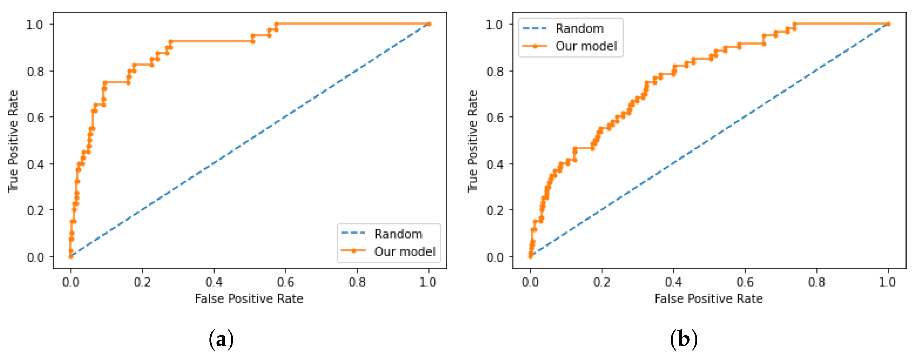
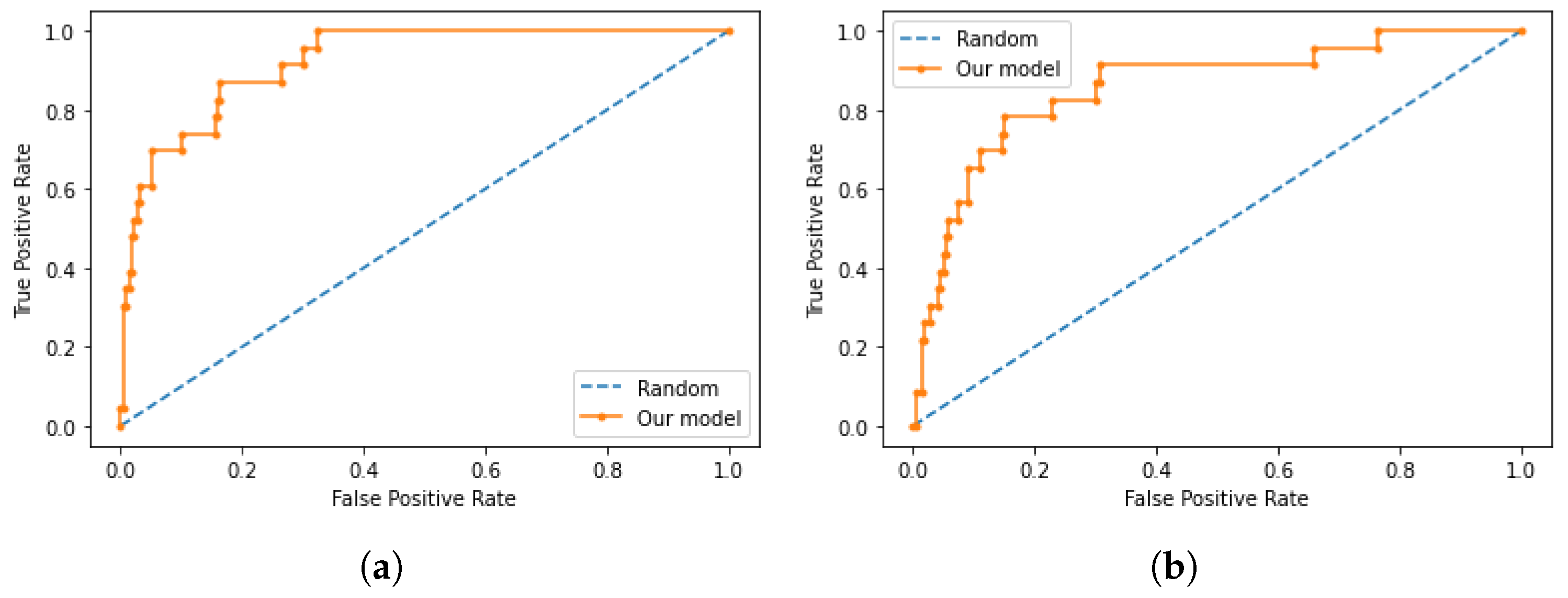
2.5. Results

In this section, the performance of the final meta-model in the validation set is presented. To quantify the performance, the Receiver Operating Characteristic (ROC) curve and the Precision-Recall (PR) curves are used. The ROC curves for 24 and 48 h forecasting are shown in Figure 2a and Figure 2b, respectively. The solid curves show the model performance of true positive rate as the false positive rate is changed by varying thresholds across the predicted score. The model performs considerably better than a random model (dashed lines), where the prediction is distributed according to the frequency of majority events (no-frost days). Due to the highly unbalanced dataset, PR curves are also created to establish performance against the minority events. The results for 24 and 48 h forecasting are shown in Figure 3a and Figure 3b, respectively. It can be noticed that even though the model presented in the paper is better than a minority frequency-based random model, in general, there is a large trade-off between precision and recall. Moreover, understandably, 48 h forecasting performs worse than 24 h ahead prediction as meteorological and climate fluctuations play a bigger part in the 48 h ahead prediction. It should be noted that sudden changes in the ROC and PR curves are the result of the smallness of the minority class sample size.
Next, the model performance is discussed on the test dataset taken from weather stations in the areas of interest. By comparing the ROC curves of prediction from the test dataset (Figure 4) to that of the validation set (Figure 2), it can be seen that the model performances are alike, if not better. A similar conclusion can also be drawn by looking into the PR curves in Figure 2.
A similar conclusion can also be drawn by looking into the PR curves in Figure 5. To look into the cases of false positives and false negatives, from the validation set, optimal thresholds are selected by maximizing the F 2 -score or J-statistics. F 2 -score, instead of the more ubiquitous F 1 -score, is considered the recall is more important than precision as failing to predict a frost event can be more costly than having false positives. For each threshold, three different performance indices are considered:
Recall = T P T P + F N , Precision = T P T P + F P and Balanced Accuracy = 1 2 T P T P + F N + T N T N + F P , where T P = True Positive , F P = False Positive , F N = True Negative and T N = True Negative. Under different threshold conditions, the performance indices are shown in Table 1. As is clear from the PR curves, there is a trade-off between precision and recall. As a result, depending on the cost of false positives and the type of frost protection measure, one needs to decide on the thresholds.

3. Conclusions

In conclusion, this paper develops and tests an ensemble-based meta-model for 24 and 48 h ahead frost prediction using inputs from meteorological stations located in the AoIs.The model performance shows a trade-off between precision and recall. In the case of frost prediction, depending on the type of protection measure taken, eliminating false negatives can be more important than false positives. Hence, recall is given more weight in the performance evaluation. The 24 h ahead prediction is found to be better than the 48 h one. In future work, a better model can be created by including data from a variety of weather stations near AoIs and also including ground truth data on frost events. Additionally, shifting the forecasting time towards night can lead to better performance as radiative frost in the AoIs happens in the early morning. Complimenting the weather data with more variables such as evapotranspiration and cloud coverage can also potentially lead to better prediction of frost events.

Author Contributions

Conceptualization, O.D. and F.R.; methodology, O.D.; software, O.D.; validation, O.D.; formal analysis, O.D.; investigation, O.D. and F.R.; resources, O.D. and F.R.; data curation, O.D. and F.R.; writing—original draft preparation, O.D.; writing—review and editing, O.D. and F.R.; visualization, O.D.; supervision, O.D.; project administration, F.R. All authors have read and agreed to the published version of the manuscript.

Funding

This research was funded by European Union’s Horizon 2020 research and innovation programme under grant agreement No. 825355.

Institutional Review Board Statement

Not applicable.

Informed Consent Statement

Not applicable.

Data Availability Statement

Not applicable.

Conflicts of Interest

The authors declare no conflict of interest.

References

  1. Agroseguro. Informe Sobre la Siniestralidad del Ejercicio 2021, Report of Spanish Agrarian Insurance Management Association. 2021. Available online: https://agroseguro.es/fileadmin/propietario/Home/INFORMES_SINIESTRALIDAD/WEB_0.12._Informe_TOTAL_SINIESTRALIDADES_2021_31_diciembre_2021_-_copia.pdf (accessed on 18 February 2022).
  2. Kalma, J.D.; Laughlin, G.P.; Caprio, J.M.; Hamer, P.J.C. The Bioclimatology of Frost: Its Occurrence, Impact and Protection. Adv. Bioclimatol. 1992, 2, 66–67. [Google Scholar]
  3. Georg, J.C.; Gerber, J.F. Techniques of Frost Prediction and Methods of Frost and Cold Protection; World Meteorological Organization (WMO): Geneva, Switzerland, 1978; Available online: https://library.wmo.int/doc_num.php?explnum_id=1080 (accessed on 25 January 2022).
  4. Jung, J.; Maeda, M.; Chang, A.; Bhandari, M.; Ashapure, A.; Landivar-Bowles, J. The potential of remote sensing and artificial intelligence as tools to improve the resilience of agriculture production systems. Curr. Opin. Biotechnol. 2021, 70, 15. [Google Scholar] [CrossRef] [PubMed]
  5. Liakos, K.G.; Busato, P.; Moshou, D.; Pearson, S.; Bochtis, D. Machine Learning in Agriculture: A Review. Sensors 2018, 18, 2674. [Google Scholar] [CrossRef] [PubMed] [Green Version]
  6. Noh, I.; Doh, H.-W.; Kim, S.-O.; Kim, S.-H.; Shin, S.; Lee, S.-J. Machine Learning-Based Hourly Frost-Prediction System Optimized for Orchards Using Automatic Weather Station and Digital Camera Image Data. Atmosphere 2021, 12, 846. [Google Scholar] [CrossRef]
  7. Ghielmi, L.; Eccel, E. Descriptive models and artificial neural networks for spring frost prediction in an agricultural mountain area. Comput. Electron. Agric. 2006, 54, 101. [Google Scholar] [CrossRef]
  8. Diedrichs, A.L.; Bromberg, F.; Dujovne, D.; Brun-Laguna, K.; Watteyne, T. Prediction of Frost Events Using Machine Learning and IoT Sensing Devices. IEEE Internet Things J. 2018, 5, 4589. [Google Scholar] [CrossRef] [Green Version]
  9. Ding, L.; Noborio, K.; Shibuya, K. Modelling and learning cause-effect—Application in frost forecast. Procedia Comput. Sci. 2020, 176, 2264. [Google Scholar] [CrossRef]
  10. Hernan, L.; Martí, L.; Sanchez-Pi, N. Frost forecasting model using graph neural networks with spatio-temporal attention. In Proceedings of the AI: Modeling Oceans and Climate Change Workshop at ICLR, Santiago, Chile, 7 May 2021. [Google Scholar]
  11. Dreisiebner-Lanz, S.; Bilavcik, A.; Chaloupka, R.; Ga̧stoł, M.; McCallum, S.; Miranda, C. MINIPAPER 04: Use of Chemicals to Help Plants Tackle Frost Damages. EIP-AGRI Focus Group. 2019. Available online: https://ec.europa.eu/eip/agriculture/sites/default/files/fg30_mp4_chemicals_frost_protection_v2.pdf (accessed on 2 February 2022).
Figure 1. Distribution of frost days in Belgida and Carlet. Each season consists of December to March. (a) Carlet, (b) Belgida.
Chemproc 10 00070 g001
Figure 2. ROC curves for the model presented in the article for the validation dataset. (a) 24 h forecasting, (b) 48 h forecasting.
Chemproc 10 00070 g002
Figure 3. PR curves for the model presented in the article for the validation dataset. (a) 24 h ahead prediction, (b) 48 h ahead prediction.
Chemproc 10 00070 g003
Figure 4. ROC curves for the test dataset. (a) 24 h forecasting, (b) 48 h forecasting.
Chemproc 10 00070 g004
Figure 5. PR curves for the test dataset. (a) 24 h ahead prediction, (b) 48 h ahead prediction.
Chemproc 10 00070 g005
Table 1. Various performance indices for 24 and 48 h ahead predictions based on the test dataset.
ForecastingThresholdRecallPrecisionBalanced Accuracy
24 h ahead F 2 -score0.870.310.83
24 h aheadJ-statistics0.740.390.81
48 h ahead F 2 -score0.830.250.78
48 h aheadJ-statistics0.560.450.75
Publisher’s Note: MDPI stays neutral with regard to jurisdictional claims in published maps and institutional affiliations.

