Review

Deep Learning for Raman Spectroscopy: A Review

1
Institute of Physical Chemistry, Friedrich Schiller University Jena, Helmholtzweg 4, 07743 Jena, Germany
2
Department of Photonic Data Science, Leibniz Institute of Photonic Technology, Albert-Einstein-Straße 9, 07745 Jena, Germany
3
Leibniz Centre for Photonics in Infection Research, 07743 Jena, Germany
*
Author to whom correspondence should be addressed.
Analytica 2022, 3(3), 287-301; https://doi.org/10.3390/analytica3030020
Submission received: 23 May 2022 / Revised: 25 June 2022 / Accepted: 29 June 2022 / Published: 19 July 2022

Abstract

:
Raman spectroscopy (RS) is a spectroscopic method which indirectly measures the vibrational states within samples. This information on vibrational states can be utilized as spectroscopic fingerprints of the sample, which, subsequently, can be used in a wide range of application scenarios to determine the chemical composition of the sample without altering it, or to predict a sample property, such as the disease state of patients. These two examples are only a small portion of the application scenarios, which range from biomedical diagnostics to material science questions. However, the Raman signal is weak and due to the label-free character of RS, the Raman data is untargeted. Therefore, the analysis of Raman spectra is challenging and machine learning based chemometric models are needed. As a subset of representation learning algorithms, deep learning (DL) has had great success in data science for the analysis of Raman spectra and photonic data in general. In this review, recent developments of DL algorithms for Raman spectroscopy and the current challenges in the application of these algorithms will be discussed.

1. Introduction

In 1928, a new scattering effect was discovered by C. V. Raman [1]. Today, this effect is called Raman scattering, which is the inelastic scattering of photons on a quantized system such as the vibrational states within molecules, e.g., in matter. Because the vibrational states of a molecule are molecule-specific, a Raman spectrum can be used as a “vibrational fingerprint” of the molecule. If Raman spectroscopy is applied to molecule mixtures, the Raman spectrum can be used as fingerprint of the respective sample [2]. Due to the intrinsic low quantum efficiency of the Raman effect, the measurement of high-quality Raman spectra requires long measurement times. Therefore, enhancement techniques, such as coherent anti-Stokes Raman spectroscopy (CARS) [3] and surface-enhanced Raman spectroscopy (SERS) [4], were invented. Nowadays, Raman spectroscopy has already widely spread into different research fields, for example, forensic analysis [5], pharmaceutical product design [6], material identification [7], disease diagnosis [8], etc. Most of the presented and similar studies employ the unlabelled version of Raman spectroscopy. For this reason, data modelling is always necessary for interpreting the untargeted spectral data [9].
The research field of applying mathematical and statistical methods on the data of chemical measurements has been defined as chemometrics by Kowalski in 1975 [10]. Usually, chemometrics for Raman spectroscopy can be divided into two main parts: data pre-processing and data modelling. In terms of data pre-processing, there are correction steps, including spike correction, wavenumber calibration, baseline correction, etc. [2]. Different pre-processing methods exist, such as traditional pre-processing, e.g., the Vancouver Raman algorithm [11], as well as machine learning options, such as automatic Raman spectra correction [12]. In terms of data modelling, machine learning (ML) models are prevailing, especially the partial least squares (PLS) algorithm. For instance, Goetz et al., used a PLS-based multivariate technique to quantify body chemicals [13]; Hedegaard et al., combined PLS and K-means clustering to identify isogenic cancer cells [14]; and Guo et al., modified PLS and principal component analysis (PCA) to improve Raman spectroscopy classification [15]. Besides, other classical machine learning algorithms are also often used for data modelling. For example, Manoharan et al., determined 12 principal components of 61 Raman spectra for breast cancer diagnosis by singular value decomposition (SVD) [16]; Widjaja et al., applied support vector machine (SVM) into near-infrared (NIR) Raman spectroscopy for classifying colonic tissue specimens [17]; and Seifert proved that random forests are efficient for analysing complex biological samples based on SERS data [18].
Apart from the afore-mentioned examples of classical machine learning models, there is a kind of representation learning, which is most often based on very deep multilayer perceptrons (MLPs). This kind of representation learning is called deep learning and it can solve various artificial-intelligence tasks [19] (pp. 1–12). With the rapid development of computer science, deep learning has changed numerous traditional research fields, including photonics [20], chemistry [21], and biology [22]. For Raman spectroscopy, deep learning models are also very helpful in both data pre-processing and data modelling, which, theoretically, can be applied to all kinds of Raman spectral data. If a large number of Raman spectra are available, they can be sent directly into deep learning models without pre-processing. It should be noted here that it is not clear what is a large number for a given DL model and application. That is, mainly, because no sample-size planning (SSP) algorithm exists for deep learning. If Raman spectra are utilized without pre-processing, the DL model should do that implicitly beside the classification or regression task. If there are different Raman experiments, the models can be retrained or just directly used for a new experiment or task. Besides, typical deep learning algorithms in this field are convolutional neural networks (CNNs), residual networks (ResNets), recurrent neural networks (RNNs), autoencoders, and generative adversarial networks (GANs). Therefore, in the following sections, these algorithms, their recent applications in Raman spectroscopy, as well as their current challenges, will be discussed in more detail.
In this article, Section 1 has introduced the background information about Raman spectroscopy and deep learning; Section 2 will make an overview of several common deep learning models, including CNNs, ResNets, RNNs- and GANs; and Section 3 will discuss recent applications of deep learning in combination with Raman spectroscopy. The applications are grouped into four categories. Section 4 will summarise the existing challenges of deep learning for Raman spectroscopy. Finally, Section 5 will draw a conclusion.

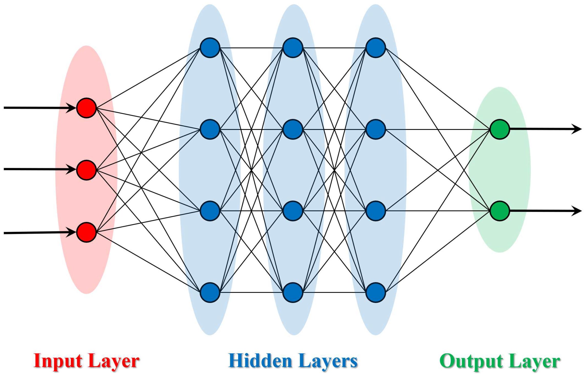
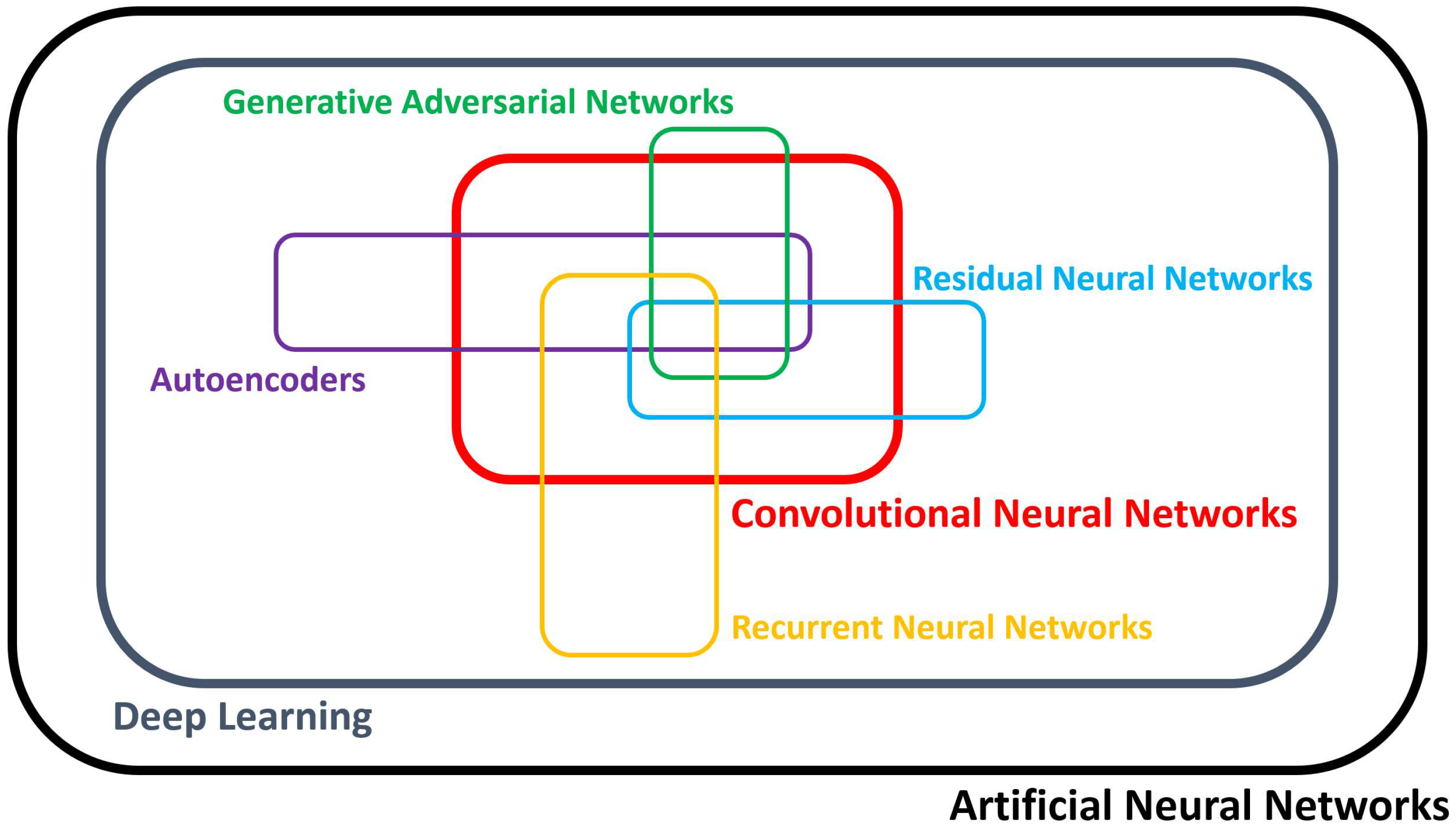
2. Deep Learning—Overview

In 1986, Rina Dechter introduced the term “deep learning” into the machine learning community [23]. Because of the recent rise of big data, deep learning (DL) has successfully infiltrated nearly all major areas of scientific research. DL belongs to the representation learning subset of artificial intelligence (AI). Most often, feedforward neural networks (FNNs) are the fundamental basis of deep learning algorithms, which are a kind of artificial neural networks (ANNs) that always consist of an input layer, hidden layers, and an output layer. The input layer sends the input data into the network, then the neurons in hidden layers process the data depending on their weights, and, finally, the processed data is returned by the output layer. The weights and bias of the network are typically updated using backpropagation and gradient-based optimization techniques. The basic architecture of an FNN is shown in Figure 1. This architectural basis makes it possible for a deep learning network to be capable of representing functions of increasing complexity by adding more units and layers [19] as long as sufficient large numbers of labelled training samples are available. Based on this basic architecture, various deep learning-based algorithms have been recently invented and implemented, for example, CNNs, ResNets, RNNs, autoencoders, GANs, etc, [9]. Their relationships are illustrated in Figure 2. Although these algorithms vary from one to another, an optimisation method, a cost function, a dataset, and a model defined by its building blocks, e.g., layers, are always the four fundamental components [9]. These typical deep learning algorithms will be briefly introduced in the following.

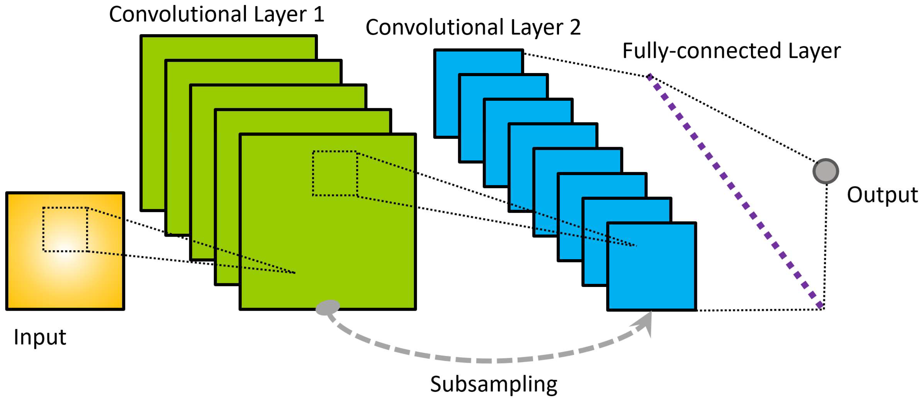
2.1. Convolutional Neural Networks (CNN)

In 1989, LeCun et al., firstly introduced the CNN for handwritten zip code recognition [24]. The most important part of a CNN is its convolutional layer. Additionally, batch normalization layers and pooling layers as well as fully-connected layers are also commonly utilized in a CNN. The input of a convolutional layer is convolved by the kernels of a convolutional layer and passed to the next layer acting as input for that layer. During the process of weight updating, the convolution kernel of each layer is learned, thus, feature maps which are generated by the kernels are updated. Additionally, pooling layers are utilized to reduce data dimension and computational complexity by subsampling. There are two most common types of pooling methods: max pooling and average pooling. Usually, a fully-connected layer is at the end of a CNN, which connects every single neuron of its previous layer to the output. Figure 3 illustrates the typical structure of a CNN model. It should be noted here that CNNs have two special concepts: parameter sharing and local connectivity. These concepts reduce the number of parameters and make the computations more efficient.

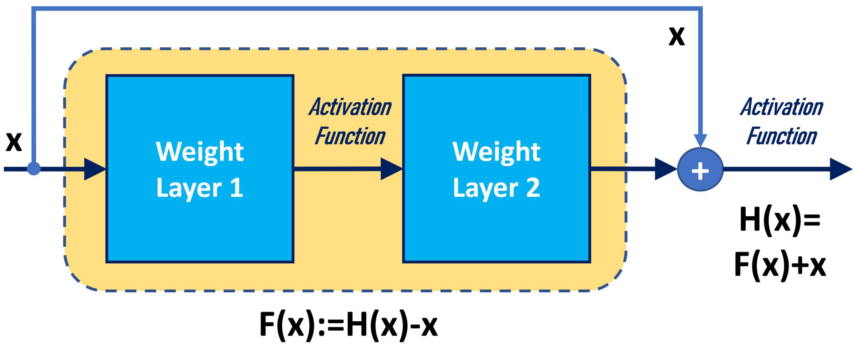
2.2. Residual Network (ResNet)
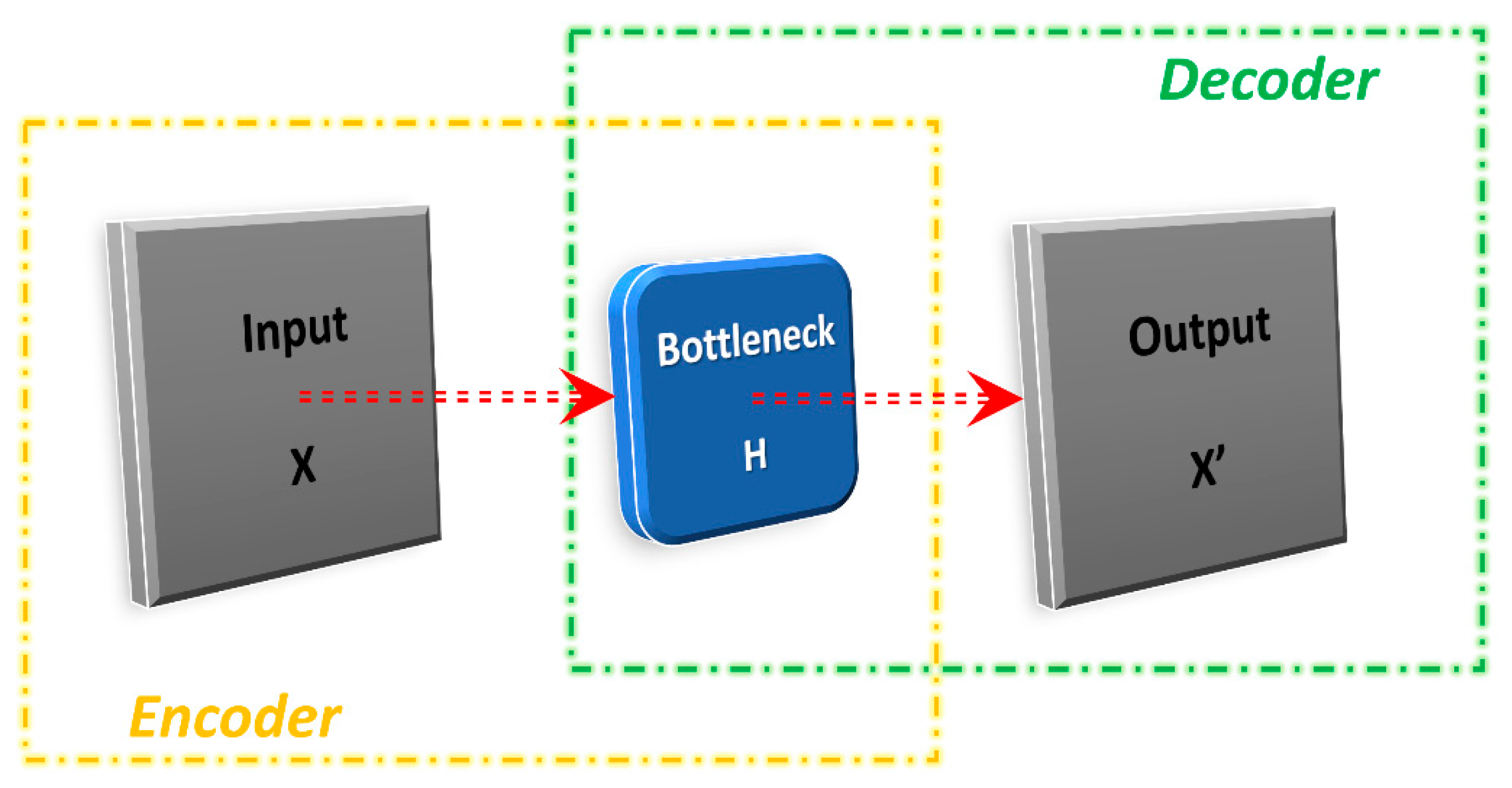
In 2015, He et al., published a paper to use residual learning for image recognition [25]. This is the first application of ResNet, containing a 34-layer network architecture. The core structure of a ResNet is its residual block, which is shown in Figure 4. The residual block utilises a shortcut to jump over layers. This design can avoid the vanishing gradient problem, which might completely stop the neural network from further learning in the training process. According to the network length, the most commonly used ResNets are ResNet-50, ResNet-101, and ResNet-152, which can be categorized as CNN variants.

2.3. Autoencoder

Unsupervised learning can be realised with an autoencoder, which has a bottleneck structure, as shown in Figure 5. An autoencoder has two main parts: an encoder and a decoder, which are designed for input and output data, respectively. The data flows from the input through a bottleneck, which forms a feature representation of the input data to model the output. An important application of an autoencoder structure constructed by means of a CNN is the U-Net, which was firstly introduced by Ronneberger et al., for biomedical image segmentation [26].

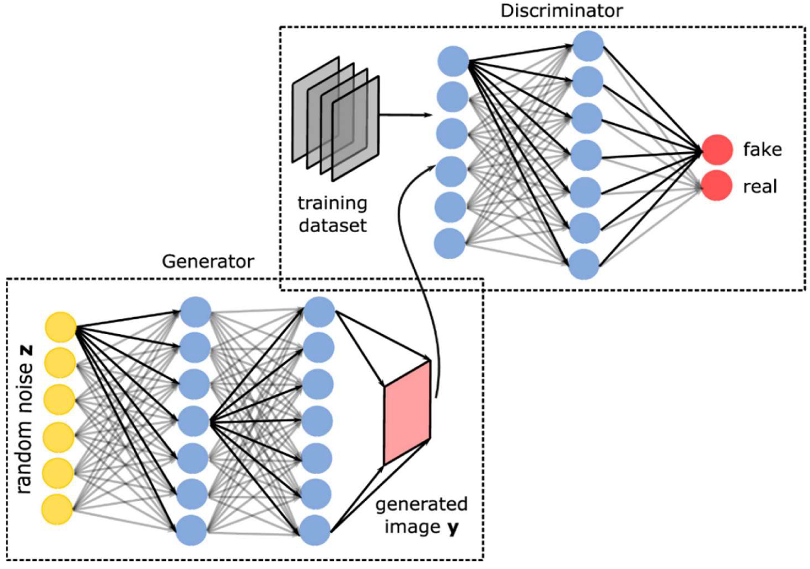
2.4. Generative Adversarial Network (GAN)

Goodfellow et al., introduced a very interesting deep learning architecture called generative adversarial network (GAN), which consists of a generator G and a discriminator D [27]. During the process of training, G aims to maximise the probability of D making a mistake, while D wants to separate real from generated data instances. The training is performed sequentially using the minimax loss, which is, actually, a minimax two-player game. As a result, G learns to generate data that comes from on approximated distribution similar to the distribution of the original input. Meanwhile, D try to distinguish real images in the training dataset between generated fake images. Figure 6 shows a typical GAN architecture.

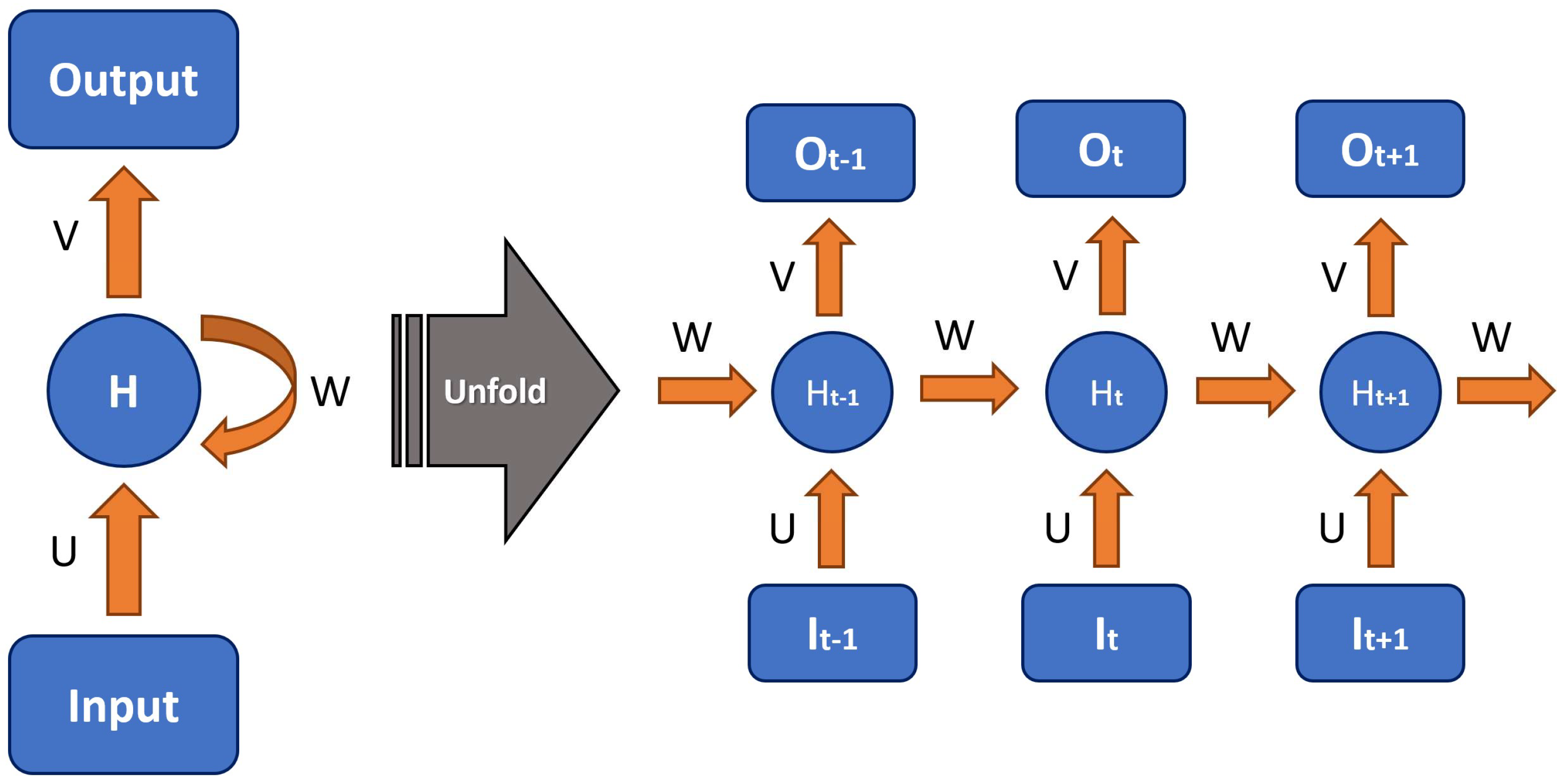
2.5. Recurrent Neural Network (RNN)

In 1997, Hochreiter and Schmidhuber invented the long short-term memory (LSTM) network, which is a form of a RNN [28]. LSTM networks have feedback connections, so they are able to process entire sequences of data and avoid the vanishing gradient problem. RNNs are capable of adding memory to the network over time, thus, they have succeeded widely in time-series processing, such as speech signal recognition. More specifically, according to Pradhan et al., RNN architectures can be separated into three groups: many-to-one architecture, one-to-many architecture, and many-to-many architecture [9]. The way of unfolding a basic RNN is shown in Figure 7.

3. Recent Applications for Raman Spectroscopy

Classical machine learning techniques have been widely used for Raman spectroscopy. Generally, data pre-processing, feature extraction (or feature selection), and data modelling are necessary steps. On the contrary, with deep learning, the workload of such complicated steps can all be done by a single neural network on condition that there exist sufficient training data. Based on the output types, deep learning applications for Raman spectroscopy can be separated into four main parts: pre-processing, classification, regression, and highlighting, which are shown in Figure 8. After model training using a Raman spectrum as input, a pre-processing model outputs another Raman spectrum (usually filtered or denoised); a classification model outputs a label; a regression model outputs a number or probabilistic value; and a highlighting model divides the input into different parts and usually outputs a certain region of interest (ROI) of the 1D spectral data. In this section, recent achievements about these major applications will be introduced, as demonstrated in Table 1.

3.1. Pre-Processing

As mentioned above, because the Raman effect is a weak effect, it can be easily contaminated by noise and other corrupting effects. Thus, pre-processing is, traditionally, a must. According to Bocklitz et al., and Guo et al., after getting raw spectra, spike correction, wavenumber calibration, intensity calibration, baseline correction, and spectral smoothing, spectral normalisation as well as dimension reduction are always needed [2,29]. Because the computational complexity of the above-mentioned pre-processing sequence is high, and simply no universal pre-processing technique exists, the definition and implementation of the pre-processing (sequence) becomes a heavy burden [30]. Besides, there does not exist standard pre-processing protocol for different laboratories and devices, and some pre-processing sequences could be inappropriate [2]. Due to these facts, it is of vital importance to find another way to solve the pre-processing challenge. Luckily enough, recent research results have shown that deep learning is a powerful alternative for Raman spectral pre-processing.
1D CNNs are commonly applied for Raman spectral pre-processing. For example, Wahl et al., presented a single-step automated Raman spectral pre-processing method using CNN [31]. In this method, signal peaks, baselines, and background noise are, firstly, randomly added in order to create synthetic spectra. After that, a CNN model is trained for mapping a set of input Raman spectra to the corresponding ideal spectrum. This CNN model consists of a feature extraction block (four convolutional layers followed by batch normalization and rectified linear unit (ReLU) layers; the first two are also followed by average pooling layers) as well as a regression block (a dropout layer, a fully-connected layer, and a regression layer). As a result, most pre-processed outputs had better signal quality under these three criteria: root mean square error (RMSE), structural similarity index measure (SSIM), and signal-to-noise ratio (SNR). Additionally, Valensise et al., also implemented a 1D CNN model to remove non-resonant background (NRB) from broadband coherent anti-Stokes Raman scattering (B-CARS) spectra [32], as demonstrated in Figure 9. This model is called SpecNet, which consists of five convolutional layers followed by three fully-connected layers. The convolutional layers have 128, 64, 16, 16, and 16 filters, respectively; the fully-connected layers have 32, 16, and 640 neurons, respectively, and each layer has a rectified linear unit (ReLU) as activation function. After going through this model, the distorted line shapes and the degraded chemical information can be corrected, so that the analysis of B-CARS spectra can be greatly simplified and accelerated.
Apart from the above-mentioned basic 1D CNNs, autoencoders and ResNets are also widely used for Raman spectral pre-processing. A very typical example is the 1D ResUNet implemented by Horgan et al., which is designed for the process of Raman spectral denoising [33]. In their study, MDA-MB-231 breast cancer cells were cultured to obtain both low SNR (0.1 s integration time per spectrum) and high SNR (1 s integration time per spectrum) Raman spectra, so that the 1D ResUNet could then be trained for enhancing the low SNR ones. This model has 20 convolutional layers, each of them is with a ReLU layer, and they make up five residual blocks consisting of an encoder and a decoder. In addition, Gebrekidan et al., used a similar ResUNet model to efficiently remove noise and background from raw Raman spectra to increase signal quality [34]. The encoder of this ResUNet consists of four repeated sequences (each has two 5 × 1 convolutional layers, one batch normalization layer, and one max-pooling layer) followed by two 5 × 1 convolutional layers; the decoder of this ResUNet also consists of four repeated sequences (each has two 5 × 1 convolutional layers, one up-sampling layer, and one concatenation layer), followed by a 1 × 1 convolutional layer at the end.
Some other impressive studies about deep learning for Raman pre-processing have also been developed by researchers. For example, Pan et al., used a CNN with seven 2-dimentional convolutional layers (each has 100 filters of the size 100 × 1 and is followed by a 100-channel batch normalization layer, a ReLU layer, and a max-pooling layer) and one fully-connected layer at the end [35]; Houhou et al., compared a long short-term memory network (LSTM) made up of the input gate, the forget gate, the output gate, and the cell state with maximum entropy method (MEM) and Kramers-Kronig relation (KK) for CARS phase retrieval, which performs well and does not need background removal in advance [36].

3.2. Classification and Regression

To the best knowledge of the author, most applications of deep learning algorithms for Raman spectroscopy are usually about spectral classification. When the output of a deep learning algorithm is a value describing the (estimated) probability of belonging to a certain class, it can be seen as a regression problem. If a classification threshold is added to such a regression algorithm, then it can become a classification algorithm. Therefore, in most applications, classification and regression are usually mixed in practice. So, these two types of applications will be introduced together in this section. 1D CNNs are the most commonly applied models among these algorithms, and ResNets are very popular as well. Most of the studies train the model from the very beginning, while few use transfer learning to simplify the weight-updating process and to adapt to the small dataset size. Usually, these deep learning-based Raman spectral classification models feature good test performances in terms of their accuracies or receiver operating characteristic (ROC) curves. In the following, a number of recent classification examples are summarised.
Same as pre-processing, 1D CNNs also play a very important role in Raman spectral classification. For example, to distinguish human and animal blood, Dong et al., used a simplified network modified from LeNet-5 architecture with only two convolutional layers for feature extraction followed by one fully-connected layer for classification, which achieved an accuracy of 96.33% [37]; to detect prostate cancer, Lee et al., used another 1D CNN for Raman spectra from extracellular vesicles (EVs) [38]; to assess the disease activity of ulcerative colitis (UC), Kirchberger-Tolstik et al., used a 1D CNN as well and reached a mean sensitivity of 78% and a mean specificity of 93% for the four Mayo endoscopic scores [39]. Besides, an accuracy of 93% has been reached for classifying lymph node carcinoma of the prostate (LNCaP), prostate cancer cell line (PC3), and red blood cell (RBC) and platelet. This model does not require any external data pre-processing step, its three convolution-max pooling layers extract features from spectral data, and then its four fully-connected layers output classification labels at the end of neural network. To detect microbial contamination, Maruthamuthu et al., used a 1D CNN for distinguishing Raman spectra of Chinese hamster ovary (CHO) cells from 12 types of microbes, which achieved the accuracy of 95–100% after training by Adam optimizer and the five-fold leave-one-out cross-validation (LOOCV) strategy [40]. This model is composed of three parts: an initial convolutional layer with the kernel size of 7 (followed by a batch normalization layer and a ReLU layer), eight residual blocks with the kernel size of 3 and a fully-connected layer at the end. To identify materials rapidly, Boonsit et al., implemented a 1D CNN as well for low-resolution Raman spectra collected from NaNO3, BaSO4, Ba(NO3)2, KNO3, Pb(NO3)2, and CH4N2O, and the accuracy of which was found to be 96.7% [7]. This model consists of four convolutional blocks (each contains a convolutional layer, a ReLU layer, and a max-pooling layer) for feature extraction and one output layer for spectral classification. Apart from the above, a 1D CNN composed of only two convolutional layers was applied into a nanoplasmonics biosensing chip (NBC) by Cheng et al., which could correctly identify 91% of the 100 spectra on validation dataset for hepatocellular carcinoma (HCC) or healthy patients [41]. The two convolutional layers of this model are with 8 or 16 kernels of the size 3 × 1, respectively. A batch normalization layer is attached to each convolutional layer, and a 2-by-1 max-pooling layer additionally follows the first convolutional layer. At the end, a concatenate layer, a fully-connected layer as well as a softmax function are used for outputting the classification results. Furthermore, a novel approach called “deep learning-based component identification” (DeepCID) was invented by Fan et al., for successfully detecting 167 types of pure components (methanol, ethanol, acetonitrile, etc.) based on Raman spectral information [42], as illustrated in Figure 10. DeepCID is a four-layer CNN model consisting of two convolutional layers (each with a 5 × 1 convolutional kernel and a 2-by-1 max-pooling operation) and two fully-connected layers. As a result, DeepCID achieved an accuracy of 98.8% for all 167 components and 160 of them achieved 99.5%. Because of this satisfying result, the non-negative least squares (NNLS) algorithm and DeepCID were later combined by Fu et al., which also worked impressively well in their lactose-dominated drug (LLD) quantitative model [43].
Apart from the 1D CNN algorithms in the above, autoencoders and ResNets are also quite popular for Raman spectral classification. For example, in terms of autoencoder, Houston et al., combined one with a locally connected neural network (LCNN) to create a two-step classification model for being accurate and robust in the presence of negative outliers [44]. In this model, the LCNN was designed for training data, while the autoencoder was utilised for outlier detection. In terms of ResNet, Ho et al., implemented one network with 25 convolutional layers for rapid bacteria identification [45]. The antibiotic treatment identification accuracies of their model were 97.0 ± 0.3%. In addition, a new framework entitled “diverse spectral band-based deep residual network” (DSB-ResNet) was proposed by Ding et al., which had the best performance of detecting tongue squamous cell carcinoma (TSCC) with 97.38%, 98.75%, and 98.25% for sensitivity, specificity, and accuracy, respectively [46]. DSB-ResNet has a global convolution and slice (CS) layer after input, and then is equally divided into four quarters. The outputs of the CS layer and four quarters are sent into five 34-layer ResNets, respectively, which are followed by a concatenation and dropout layer and a fully-connected layer before the final output. Additionally, another new framework using residual blocks named “multi-feature fusion convolutional neural network” (MCNN) was designed by Chen et al., which had the highest accuracy among its competitors for thyroid dysfunction diagnosis with serum Raman spectra collected from 199 patients [47]. MCNN has three 1D convolutional layers immediately after the input, and these three layers also contain two residual blocks. The fourth layer of MCNN is a concatenate layer, which is followed by a flatten layer as well as two fully-connected layers before the final softmax output layer.
There are many other types of CNN-related algorithms for Raman spectroscopic classification in the research field as well. For example, an optimal Scree-CNN model was implemented for classifying salivary NS1 SERS spectra with 100% accuracy [48]. This Scree-CNN consists of a feature extraction part and a classification part. The feature extraction part contains an input layer, a convolutional layer, and a ReLU layer; the classification part contains a multilayer perceptron (MLP) and a softmax output layer. Besides, Pan and his colleagues even increased the Raman data dimension from 1D to 2D by wavelet transform before classification [49,50]. In addition, a single-layer multiple-kernel-based convolutional neural network (SLMK-CNN) containing one convolutional layer with five different kernels, one flatten layer, and two fully-connected layers was created for Raman spectra obtained from porcine skin samples [51]. Notably, for pathogen classification, Yu et al., even combined Raman spectroscopy with GAN to achieve high accuracy when the training dataset size is limited [52]. In their GAN model, the generator G (a multilayer perceptron) worked for data augmentation and the discriminator D (a multilayer deep neural network) acted as a classifier.
When it comes to the limitation of dataset size, some other researchers have shown that using transfer learning is very helpful to the training process of classification models for Raman spectroscopy. For example, Thrift and Ragan tried a CNN-based single molecule SERS quantification method that transferred the knowledge from Rhodamine 800 (R800) domain to methylene blue (MB) domain. Their SERS quantification method could be highly satisfactory even with only 50 new MB training samples [53]. Their CNN model is inspired from the classic LeNet architecture, which begins with an entry flow of four convolutional layers followed by two max-pooling layers, respectively, and ends with an exit flow of a flatten layer, a dropout layer and two fully-connected layers. Furthermore, Zhang et al., pretrained a source dataset made of Bio-Rad and RRUFF databases and increased their CNN classification accuracy by 4.1% with just 216 new spectra from the target dataset [54]. However, these applications of transfer learning greatly depend on a spectroscopic source dataset, therefore the feasibility of using more general source datasets (e.g., ImageNet) still remains to be analysed.

3.3. Spectral Data Highlighting

As introduced above, most deep learning models can directly predict the classes of Raman spectra in a classification approach or predict continuous values, even without pre-processing and spectral highlighting, consequently, the need of highlighting important regions of spectra is not that high. Therefore, spectral data highlighting is not that often seen for Raman spectroscopy as the three afore-mentioned application scenarios. But there exist a few studies on the topic, e.g., answering the question of which spectral features are important for a given task. To give an instance, Fukuhara and his team highlighted the important regions of a given Raman spectrum by a CNN [55]. This CNN begins with two convolutional blocks (each has a convolutional layer followed by a max-pooling layer) and ends with two fully-connected layers. In their model, Raman peaks were extracted, and near-zero feature values at background region were obtained. From another perspective, the Raman spectral highlighting task can as well be considered as the supplement or preparation for pre-processing steps. Therefore, further research about deep learning algorithms purely for Raman spectral highlighting still needs to be conducted.
Table 1. Examples of typical deep learning applications for Raman spectroscopy.
ApplicationExamples
Pre-processingWahl et al. [31], Valensise et al. [32], Horgan et al. [33], Gebrekidan et al. [34], Pan et al. [35], and Houhou et al. [36]
Classification/
Regression
Boonsit et al. [7], Dong et al. [37], Lee et al. [38], Kirchberger-Tolstik et al. [39], Maruthamuthu et al. [40], Cheng et al. [41], Fan et al. [42], Fu et al. [43], Houston et al. [44], Ho et al. [45], Ding et al. [46], Chen et al. [47], Saifuzzaman et al. [48], Pan et al. [49,50], Sohn et al. [51], Yu et al. [52], Thrift and Ragan [53], and Zhang et al. [54]
HighlightingFukuhara et al. [55]

4. Challenges and Shortcomings

Although deep learning has already improved Raman spectroscopic research, there still exist many challenges connected with the application of deep learning for Raman spectra. The most important issue is about training and data preparation. First of all, deep learning algorithms are highly data-demanding, but it is quite hard to acquire large sets of (independent) Raman spectroscopic data. Therefore, small sample sizes of Raman datasets might lead to low algorithm performance. Secondly, currently there no large open-source Raman spectroscopic dataset exists to pre-train DL models for transfer learning, and the effectiveness of using more general datasets, such as ImageNet, still remains unknown. Thirdly, the generalisation ability of the trained models is questionable, because a model that performs quite well on one dataset might produce disappointing results on another dataset due to overfitting. Last but not least, because Raman spectra are often of low quality and contaminated with noise, extra pre-processing and enhancing steps are often needed, which increase the complexity of data analysis.

5. Conclusions

As introduced above, deep learning is a representation learning method and it has been widely used in the research field of Raman spectroscopy, especially during recent years. Generally, there are different (and often applied) deep learning models, such as CNNs, ResNets, autoencoders, GANs, RNNs, etc, which were introduced in this contribution. We grouped the applications of these models into four major Raman spectroscopic application scenarios where these models are usually implemented: pre-processing, classification, regression, and (spectral) segmentation. The two most common applications are pre-processing and classification, and the least common application is Raman spectral segmentation/variable highlighting. In terms of Raman spectroscopy, segmentation often merely plays a preparatory role before pre-processing or classification steps. Regarding pre-processing, deep learning methods have already shown the great ability to surpass their conventional counterparts, especially that the time requirement of deep learning methods is lower than their classical counterparts. Many types of 1D CNNs, especially variants of ResNets and autoencoders, are largely used for Raman pre-processing. These recent achievements are significantly helpful to the next steps of Raman spectral data analysis.
On the other hand, deep learning even makes it possible to reduce the complexity of pre-processing and allows for an automatic pre-processing solution in comparison with subjective pre-processing workflows. Some deep learning models directly combine all the pre-processing steps together with the ultimate goal, such as classification or regression, in just one single network. For these scenarios, 1D CNNs and ResNets are very popular tools as well, and sometimes GANs and autoencoders are also applied. Notably, there always exists the problem of Raman spectral dataset size limitation, thus, implementing GANs for data augmentation can be highly effective but needs further systematic research. Besides, transfer learning has become another option to avoid this data size problem by reusing the knowledge gained from source datasets of other domains. However, currently these source datasets only concentrate on Raman spectra databases, so it still remains to be analysed in respect of the feasibility of applying more general options similar to large, annotated image datasets, e.g., ImageNet.
With the rapid development of computer science, there arise more and more deep learning-related algorithms conquering other fields, but their effectiveness for Raman spectral data is unknown. In brief, although deep learning has already demonstrated its great potential for Raman spectroscopy, there are still many open questions to be answered, especially relating to the estimation of the prediction quality of deep-leaning models on small datasets with complex co-variance structures. There are other questions about the influence of GAN-based data augmentation and how transfer learning can be applied reliably for Raman spectroscopy.

Author Contributions

Literature research, R.L.; writing—original draft preparation, R.L. and T.B.; writing—review and editing, T.B. and J.P. All authors have read and agreed to the published version of the manuscript.

Funding

This work is supported by the Ministry for Economics, Sciences, and Digital Society of Thuringia (TMWWDG), under the framework of the Landesprogramm ProDigital (DigLeben-5575/10-9) and the Federal Ministry of Education and Research of Germany (BMBF), funding program Photonics Research Germany (FKZ: 13N15466, 13N15710, and 13N15708) and is integrated into the Leibniz Center for Photonics in Infection Research (LPI). The LPI initiated by Leibniz-IPHT, Leibniz-HKI, UKJ and FSU Jena is part of the BMBF national roadmap for research infrastructures.

Institutional Review Board Statement

Not applicable.

Informed Consent Statement

Not applicable.

Data Availability Statement

Not applicable.

Acknowledgments

The authors would like to thank the abovementioned funding bodies as well as the reviewers for the time and effort they spent to improve the quality of this article.

Conflicts of Interest

The authors declare no conflict of interest.

References

  1. Raman, C.V. A new radiation. Indian J. Phys. 1928, 2, 387–398. [Google Scholar] [CrossRef]
  2. Bocklitz, T.W.; Guo, S.; Ryabchykov, O.; Vogler, N.; Popp, J. Raman based molecular imaging and analytics: A magic bullet for biomedical applications!? Anal. Chem. 2016, 88, 133–151. [Google Scholar] [CrossRef] [PubMed]
  3. Maker, P.D.; Terhune, R.W. Study of optical effects due to an induced polarization third order in the electric field strength. Phys. Rev. 1965, 137, 801–818. [Google Scholar] [CrossRef]
  4. Fleischmann, M.; Hendra, P.J.; McQuillan, A.J. Raman spectra of pyridine adsorbed at a silver electrode. Chem. Phys. Lett. 1974, 26, 163–166. [Google Scholar] [CrossRef]
  5. Penido, C.A.F.O.; Pacheco, M.T.T.; Lednev, I.K.; Silveira, L., Jr. Raman spectroscopy in forensic analysis: Identification of cocaine and other illegal drugs of abuse. J. Raman Spectrosc. 2016, 47, 28–38. [Google Scholar] [CrossRef]
  6. Paudel, A.; Raijada, D.; Rantanen, J. Raman spectroscopy in pharmaceutical product design. Adv. Drug Deliv. Rev. 2015, 89, 3–20. [Google Scholar] [CrossRef] [Green Version]
  7. Boonsit, S.; Kalasuwan, P.; van Dommelen, P.; Daengngam, C. Rapid material identification via low-resolution Raman spectroscopy and deep convolutional neural network. J. Phys. Conf. Ser. 2021, 1719, 012081. [Google Scholar] [CrossRef]
  8. Ryzhikova, E.; Ralbovsky, N.M.; Sikirzhytski, V.; Kazakov, O.; Halamkova, L.; Quinn, J.; Zimmerman, E.A.; Lednev, I.K. Raman spectroscopy and machine learning for biomedical applications: Alzheimer’s disease diagnosis based on the analysis of cerebrospinal fluid. Spectrochim. Acta Part A Mol. Biomol. Spectrosc. 2021, 248, 119188. [Google Scholar] [CrossRef]
  9. Pradhan, P.; Guo, S.; Ryabchykov, O.; Popp, J.; Bocklitz, T.W. Deep learning a boon for biophotonics? J. Biophotonics 2020, 13, e201960186. [Google Scholar] [CrossRef] [Green Version]
  10. Kowalski, B.R. Chemometrics: Views and propositions. J. Chem. Inf. Comput. Sci. 1975, 15, 201–203. [Google Scholar] [CrossRef]
  11. Zhao, J.; Lui, H.; McLean, D.I.; Zeng, H. Automated autofluorescence background subtraction algorithm for biomedical Raman spectroscopy. Appl. Spectrosc. 2007, 61, 1225–1232. [Google Scholar] [CrossRef] [PubMed]
  12. Witjes, H.; van den Brink, M.; Melssen, W.J.; Buydens, L.M.C. Automatic correction of peak shifts in Raman spectra before PLS regression. Chemom. Intell. Lab. Syst. 2000, 52, 105–116. [Google Scholar] [CrossRef]
  13. Goetz, M.J., Jr.; Coté, G.L.; Erckens, R.; March, W.; Motamedi, M. Application of a multivariate technique to Raman spectra for quantification of body chemicals. IEEE Trans. Biomed. Eng. 1995, 42, 728–731. [Google Scholar] [CrossRef]
  14. Hedegaard, M.; Krafft, C.; Ditzel, H.J.; Johansen, L.E.; Hassing, S.; Popp, J. Discriminating isogenic cancer cells and identifying altered unsaturated fatty acid content as associated with metastasis status, using K-means clustering and partial least squares-discriminant analysis of Raman maps. Anal. Chem. 2010, 82, 2797–2802. [Google Scholar] [CrossRef]
  15. Guo, S.; Rösch, P.; Popp, J.; Bocklitz, T. Modified PCA and PLS: Towards a better classification in Raman spectroscopy-based biological applications. J. Chemom. 2020, 34, e3202. [Google Scholar] [CrossRef] [Green Version]
  16. Manoharan, R.; Shafer, K.; Perelman, L.; Wu, J.; Chen, K.; Deinum, G.; Fitzmaurice, M.; Myles, J.; Crowe, J.; Dasari, R.R.; et al. Raman spectroscopy and fluorescence photon migration for breast cancer diagnosis and imaging. Photochem. Photobiol. 1998, 67, 15–22. [Google Scholar] [CrossRef]
  17. Widjaja, E.; Zheng, W.; Huang, Z. Classification of colonic tissues using near-infrared Raman spectroscopy and support vector machines. Int. J. Oncol. 2008, 32, 653–662. [Google Scholar] [CrossRef] [Green Version]
  18. Seifert, S. Application of random forest based approaches to surface-enhanced Raman scattering data. Sci. Rep. 2020, 10, 5436. [Google Scholar] [CrossRef]
  19. Goodfellow, I.; Bengio, Y.; Courville, A. Deep Learning; MIT Press: Cambridge, MA, USA, 2016; pp. 1–481. ISBN 978-026-203-561-3. [Google Scholar]
  20. Ma, W.; Liu, Z.; Kudyshev, Z.A.; Boltasseva, A.; Cai, W.; Liu, Y. Deep learning for the design of photonic structures. Nat. Photonics 2021, 15, 77–90. [Google Scholar] [CrossRef]
  21. Mater, A.C.; Coote, M.L. Deep learning in chemistry. J. Chem. Inf. Model. 2019, 59, 2545–2559. [Google Scholar] [CrossRef]
  22. Ching, T.; Himmelstein, D.S.; Beaulieu-Jones, B.K.; Kalinin, A.A.; Do, B.T.; Way, G.P.; Ferrero, E.; Agapow, P.M.; Zietz, M.; Hoffman, M.M.; et al. Opportunities and obstacles for deep learning in biology and medicine. J. R. Soc. Interface 2018, 15, 20170387. [Google Scholar] [CrossRef] [PubMed] [Green Version]
  23. Dechter, R. Learning while searching in constraint-satisfaction-problems. In Proceedings of the 5th National Conference on Artificial Intelligence (AAAI-86), Philadelphia, PA, USA, 11–15 August 1986; pp. 178–183. [Google Scholar]
  24. LeCun, Y.; Boser, B.; Denker, J.S.; Henderson, D.; Howard, R.E.; Hubbard, W.; Jackel, L.D. Backpropagation applied to handwritten zip code recognition. Neural Comput. 1989, 1, 541–551. [Google Scholar] [CrossRef]
  25. He, K.; Zhang, X.; Ren, S.; Sun, J. Deep residual learning for image recognition. In Proceedings of the 2016 IEEE Conference on Computer Vision and Pattern Recognition (CVPR 2006), Las Vegas, NV, USA, 26 June–1 July 2016; pp. 1–12. [Google Scholar]
  26. Ronneberger, O.; Fischer, P.; Brox, T. U-Net: Convolutional networks for biomedical image segmentation. arXiv 2015, arXiv:1505.04597. [Google Scholar]
  27. Goodfellow, I.J.; Pouget-Abadie, J.; Mirza, M.; Xu, B.; Warde-Farley, D.; Ozair, S.; Courville, A.; Bengio, Y. Generative adversarial nets. arXiv 2014, arXiv:1406.2661. [Google Scholar]
  28. Hochreiter, S.; Schmidhuber, J. Long short-term memory. Neural Comput. 1997, 9, 1735–1780. [Google Scholar] [CrossRef]
  29. Guo, S.; Popp, J.; Bocklitz, T. Chemometric analysis in Raman spectroscopy from experimental design to machine learning-based modeling. Nat. Protoc. 2021, 16, 5426–5459. [Google Scholar] [CrossRef]
  30. Gerretzen, J.; Szymańska, E.; Jansen, J.J.; Bart, J.; van Manen, H.J.; van den Heuvel, E.R.; Buydens, L.M. Simple and effective way for data preprocessing selection based on design of experiments. Anal. Chem. 2015, 87, 12096–12103. [Google Scholar] [CrossRef] [Green Version]
  31. Wahl, J.; Sjödahl, M.; Ramser, K. Single-step preprocessing of Raman spectra using convolutional neural networks. Appl. Spectrosc. 2020, 74, 427–438. [Google Scholar] [CrossRef]
  32. Valensise, C.M.; Giuseppi, A.; Vernuccio, F.; de la Cadena, A.; Cerullo, G.; Polli, D. Removing non-resonant background from CARS spectra via deep learning. APL Photonics 2020, 5, 061305. [Google Scholar] [CrossRef]
  33. Horgan, C.C.; Jensen, M.; Nagelkerke, A.; St-Pierre, J.P.; Vercauteren, T.; Stevens, M.M.; Bergholt, M.S. High-Throughput molecular imaging via deep learning enabled Raman spectroscopy. Anal. Chem. 2021, 93, 15850–15860. [Google Scholar] [CrossRef]
  34. Gebrekidan, M.T.; Knipfer, C.; Braeuer, A.S. Refinement of spectra using a deep neural network: Fully automated removal of noise and background. J. Raman Spectrosc. 2021, 52, 723–736. [Google Scholar] [CrossRef]
  35. Pan, L.; Pipitsunthonsan, P.; Daengngam, C.; Channumsin, S.; Sreesawet, S.; Chongcheawchamnan, M. Noise reduction technique for Raman spectrum using deep learning network. arXiv 2020, arXiv:2009.04067. [Google Scholar]
  36. Houhou, R.; Barman, P.; Schmitt, M.; Meyer, T.; Popp, J.; Bocklitz, T. Deep learning as phase retrieval tool for CARS spectra. Opt. Express 2020, 28, 21002–21024. [Google Scholar] [CrossRef] [PubMed]
  37. Dong, J.; Hong, M.; Xu, Y.; Zheng, X. A practical convolutional neural network model for discriminating Raman spectra of human and animal blood. J. Chemom. 2019, 33, e3184. [Google Scholar] [CrossRef]
  38. Lee, W.; Lenferink, A.T.M.; Otto, C.; Offerhaus, H.L. Classifying Raman spectra of extracellular vesicles based on convolutional neural networks for prostate cancer detection. J. Raman Spectrosc. 2020, 51, 293–300. [Google Scholar] [CrossRef]
  39. Kirchberger-Tolstik, T.; Pradhan, P.; Vieth, M.; Grunert, P.; Popp, J.; Bocklitz, T.W.; Stallmach, A. Towards an interpretable classifier for characterization of endoscopic Mayo scores in ulcerative colitis using Raman spectroscopy. Anal. Chem. 2020, 92, 13776–13784. [Google Scholar] [CrossRef]
  40. Maruthamuthu, M.K.; Raffiee, A.H.; de Oliveira, D.M.; Ardekani, A.M.; Verma, M.S. Raman spectra-based deep learning: A tool to identify microbial contamination. Microbiol. Open 2020, 9, e1122. [Google Scholar] [CrossRef]
  41. Cheng, N.; Fu, J.; Chen, D.; Chen, S.; Wang, H. An antibody-free liver cancer screening approach based on nanoplasmonics biosensing chips via spectrum-based deep learning. Nano Impact 2021, 21, 100296. [Google Scholar] [CrossRef]
  42. Fan, X.; Ming, W.; Zeng, H.; Zhang, Z.; Lu, H. Deep learning-based component identification for the Raman spectra of mixtures. Analyst 2019, 144, 1789–1798. [Google Scholar] [CrossRef]
  43. Fu, X.; Zhong, L.; Cao, Y.; Chen, H.; Lu, F. Quantitative analysis of excipient dominated drug formulations by Raman spectroscopy combined with deep learning. Anal. Methods 2021, 13, 64–68. [Google Scholar] [CrossRef]
  44. Houston, J.; Glavin, F.G.; Madden, M.G. Robust classification of high-dimensional spectroscopy data using deep learning and data synthesis. J. Chem. Inf. Model. 2020, 60, 1936–1954. [Google Scholar] [CrossRef] [PubMed] [Green Version]
  45. Ho, C.S.; Jean, N.; Hogan, C.A.; Blackmon, L.; Jeffrey, S.S.; Holodniy, M.; Banaei, N.; Saleh, A.A.E.; Ermon, S.; Dionne, J. Rapid identification of pathogenic bacteria using Raman spectroscopy and deep learning. Nat. Commun. 2019, 10, 4927. [Google Scholar] [CrossRef] [PubMed]
  46. Ding, J.; Yu, M.; Zhu, L.; Zhang, T.; Xia, J.; Sun, G. Diverse spectral band-based deep residual network for tongue squamous cell carcinoma classification using fiber optic Raman spectroscopy. Photodiagn. Photodyn. Ther. 2020, 32, 102048. [Google Scholar] [CrossRef] [PubMed]
  47. Chen, H.; Chen, C.; Wang, H.; Chen, C.; Guo, Z.; Tong, D.; Li, H.; Li, H.; Si, R.; Lai, H.; et al. Serum Raman spectroscopy combined with a multi-feature fusion convolutional neural network diagnosing thyroid dysfunction. Optik 2020, 216, 164961. [Google Scholar] [CrossRef]
  48. Saifuzzaman, T.A.; Lee, K.Y.; Radzol, A.R.M.; Wong, P.S.; Looi, I. Optimal scree-CNN for detecting NS1 molecular fingerprint from salivary SERS spectra. In Proceedings of the 42nd Annual International Conference of the IEEE Engineering in Medicine and Biology Society (EMBC 2020), Montreal, QC, Canada, 20–24 July 2020; pp. 180–183. [Google Scholar]
  49. Pan, L.; Pipitsunthonsan, P.; Daengngam, C.; Channumsin, S.; Sreesawet, S.; Chongcheawchamnan, M. Method for classifying a noisy Raman spectrum based on a wavelet transform and a deep neural network. IEEE Access 2020, 8, 202716–202727. [Google Scholar] [CrossRef]
  50. Pan, L.; Pipitsunthonsan, P.; Daengngam, C.; Channumsin, S.; Sreesawet, S.; Chongcheawchamnan, M. Identification of complex mixtures for Raman spectroscopy using a novel scheme based on a new multi-label deep neural network. IEEE Sens. J. 2021, 21, 10834–10843. [Google Scholar] [CrossRef]
  51. Sohn, W.B.; Lee, S.Y.; Kim, S. Single-layer multiple-kernel-based convolutional neural network for biological Raman spectral analysis. J. Raman Spectrosc. 2020, 51, 414–421. [Google Scholar] [CrossRef]
  52. Yu, S.; Li, H.; Li, X.; Fu, Y.V.; Liu, F. Classification of pathogens by Raman spectroscopy combined with generative adversarial networks. Sci. Total Environ. 2020, 726, 138477. [Google Scholar] [CrossRef]
  53. Thrift, W.J.; Ragan, R. Quantification of analyte concentration in the single molecule regime using convolutional neural network. Anal. Chem. 2019, 91, 13337–13342. [Google Scholar] [CrossRef] [Green Version]
  54. Zhang, R.; Xie, H.; Cai, S.; Hu, Y.; Liu, G.; Hong, W.; Tian, Z. Transfer-Learning-Based Raman spectra identification. J. Raman Spectrosc. 2020, 51, 176–186. [Google Scholar] [CrossRef]
  55. Fukuhara, M.; Fujiwara, K.; Maruyama, Y.; Itoh, H. Feature visualization of Raman spectrum analysis with deep convolutional neural network. Anal. Chim. Acta 2019, 1087, 11–19. [Google Scholar] [CrossRef] [PubMed]
Figure 1. The basic structure of a feedforward (deep) neural network. A feedforward (deep) neural network consists of three main parts: an input layer (red units), an output layer (green units), and a number of hidden layers (blue units). The input data is sent into the network from the input layer, and then the hidden layer processes the data, which yields an output.
Analytica 03 00020 g001
Figure 2. ANN Venn diagram. This image shows that under the big ANN umbrella, CNNs, GANs, ResNets, autoencoders, and RNNs are typical deep learning models. Although they are all independent network architectures, it is very common to combine some of them together in real applications.
Analytica 03 00020 g002
Figure 3. The typical structure of a CNN. In this diagram, the yellow square (left) and the grey circle (right) represent the input data and the output data, respectively. Besides, the green and blue squares represent the first and second convolutional layers, and there is a pooling step (grey dashed arrow) in between for subsampling. Before the output, a fully-connected layer (purple dotted line) is utilised at the end of the CNN.
Analytica 03 00020 g003
Figure 4. A residual block. There is a shortcut between the input x and the desired output H(x). If the output of the nonlinear stacked layers is defined as F(x): = H(x) − x, then H(x) = F(x) + x. This network design enables a skip connection, which allows gradient information to pass through the layers and can avoid the vanishing gradient problem.
Analytica 03 00020 g004
Figure 5. The bottleneck structure of an autoencoder. The first half is an encoder (yellow), which maps the input X to the bottleneck H; while the second half is a decoder (green), which maps the bottleneck H to the output X’. Firstly, the encoder processes X and generates H (containing important features); then, the decoder translates H into the desired output X’.
Analytica 03 00020 g005
Figure 6. The typical architecture of a GAN (source: [9]). There are two parts: a generator G and a discriminator D. After enough training epochs of this minimax two-player game, G can generate high quality fake images just from random noises, and D try to distinguish real and fake images.
Analytica 03 00020 g006
Figure 7. Unfolding a basic RNN. U, V, and W are the weights of the input layer, the output layer and the hidden state, respectively; Ht, It, and Ot are the hidden state, input vector, and output result at time t, respectively. Because of the loop in RNN, gradients can flow backwards through unlimited numbers of virtual layers unfolded in space, so that they can be prevented from vanishing or exploding. And this loop also makes it possible for the RNN to process entire sequences of data.
Analytica 03 00020 g007
Figure 8. Four types of deep learning applications for Raman spectroscopy. Based on outputs, there are four types of models: pre-processing, classification, regression, and highlighting. In a pre-processing model, the output is another Raman spectrum; in a classification model, the output is a label (e.g., “healthy”); in a regression model, the output is a number or probabilistic value (e.g., “0.95”); in a highlighting model, the output is a certain spectral region of interest (ROI) of the input spectrum.
Analytica 03 00020 g008
Figure 9. An example of using 1D CNN for Raman data pre-processing (source: [32]). The visualised 1D CNN model contains three convolutional layers (blue) and two fully-connected layers (red), and it outputs a cleaned Raman spectrum.
Analytica 03 00020 g009
Figure 10. An example of using 1D CNN for Raman data classification (source: [42]). For classifying 167 different components, a set of DeepCID models with the same architecture were used. Each DeepCID model is a 1D CNN, which consists of four convolutional layers and two fully-connected layers. For training and evaluating each model, 20,000 samples were split into three datasets: training dataset, validation dataset, and test dataset.
Analytica 03 00020 g010
Publisher’s Note: MDPI stays neutral with regard to jurisdictional claims in published maps and institutional affiliations.

