Article

Design and Application of DG-FEM Basis Functions for Neutron Transport on Two-Dimensional and Three-Dimensional Hexagonal Meshes

1
Service de Génie Logiciel pour la Simulation, Université Paris-Saclay, CEA, F-91191 Gif-sur-Yvette, France
2
Service de Étude des Réacteurs et de Mathématiques Appliquées, Université Paris-Saclay, CEA, F-91191 Gif-sur-Yvette, France
3
CEA, DES, IRESNE, DTN, Cadarache, F-13108 Saint-Paul-Lez-Durance, France
*
Author to whom correspondence should be addressed.
J. Nucl. Eng. 2024, 5(1), 74-90; https://doi.org/10.3390/jne5010006
Submission received: 10 October 2023 / Revised: 29 November 2023 / Accepted: 4 January 2024 / Published: 26 February 2024

Abstract

:
Reactor design requires safety studies to ensure that the reactors will behave appropriately under incidental or accidental situations. Safety studies often involve multiphysics simulations where several branches of reactor physics are necessary to model a given phenomenon. In those situations, it has been observed that the neutron transport part is still a bottleneck in terms of computational times, with more than 80% of the total time. In the case of hexagonal lattice reactors, transport solvers usually invert the discretised Boltzmann equation by discretising the regular hexagon into lozenges or triangles. In this work, we seek to reduce the computational burden of the neutron transport solver by designing a numerical spatial discretisation scheme that would be more appropriate for honeycomb meshes. In our past research efforts, we have set up interesting discretisation schemes in the finite element setting in 2D, and we wish to extend them to 3D geometries that are prisms with a hexagonal base. In 3D, a rigorous method was derived to shrink the tensor product between 2D and 1D bases to minimum terms. We have applied these functions successfully on a reactor benchmark—Takeda Model 4—to compare and contrast the numerical results in a physical setting.

1. Introduction

With the increasing needs in electricity, nuclear energy is an appropriate option to meet supplies in a sustainable fashion. Apart from the usual designs such as Pressurised Water Reactors (PWR) which are widespread, novel nuclear reactor concepts are presently being developed throughout the world. Among those, there are technologies where the reactor core is a lattice of hexagonal assemblies: the fast neutron reactors such as sodium-cooled fast reactors (SFR) that allow for fuel regeneration or new versions of the Vodo-Vodianoï Energuetitcheski Reaktor (VVER).
Nowadays, reactor design requires safety studies to ensure that the reactors will behave appropriately under incidental or accidental situations. The safety studies often involve multiphysics simulations where several branches of reactor physics are necessary to model a given phenomenon. For instance, considering an accidental scenario such as the unprotected loss of flow (ULOF) for SFR, neutronics and thermal hydraulics are coupled together to perform a large number of parametric computations on relevant quantities pertaining to the safety of the reactor. Recently, much work has been dedicated to the coupling strategy to improve its convergence as illustrated in [1,2,3]. In the case of severe accidents, it has been observed that in these simulations, neutron transport is still a bottleneck in terms of computational times, with more than 80% of the total simulation time [4].
In the case of hexagonal lattice reactors such as SFR or VVER, transport solvers usually invert the discretised Boltzmann equation by discretising the regular hexagon into lozenges or triangles [5,6]. In fact, neutronics relies on prime quantities such as the reactivity where the accuracy is required in 1 × 10 5 or pcm, even in coarse simulations. On the other hand, the other physics coupled to neutronics would usually have more relaxed computational requirements; for instance, thermalhydraulics will consider each hexagonal assembly as a closed channel and perform independent 1D computations of this channel to provide an average assembly temperature. As such, it would seem that neutronics is “overmeshed” to guarantee proper convergence and highly resolved results.
In this work, we seek to reduce the computational burden of the neutron transport solver by designing a numerical spatial discretisation scheme which would be more appropriate for hexagonal or honeycomb meshes. In our past research efforts, we have set up interesting discretisation schemes in the finite element setting [7] in 2D, and we wish to extend those schemes to 3D geometries, which are prisms with a hexagonal base. In the first section of this work, we recall the theoretical setting of past works and use those to build an interesting and novel 3D functions. In fact, for constructing the 3D bases, we have derived a mathematical setting for keeping only the required terms from the classical tensor product between a 2D and a 1D basis sets. Then, we apply these functions on a reactor benchmark of a small SFR to compare and contrast the numerical results in a physical setting.

2. Theoretical Background

In this section, we shall provide the mathematical setting necessary to discretise the Boltzmann transport equation. First, we will talk about the usual discretisations for the energy and angle variables. Then, we shall describe the spatial discretisation in more detail for both 2D and 3D cylindrical (extruded) geometries. All the methods described in this section have been implemented in an in-house Python mock-up code.

2.1. Main Discretisations of the Transport Equation

Given a system of neutrons at equilibrium, their mean behaviour in an isotropic medium is governed by the time-independent Boltzmann transport equation, with r in a spatial domain D , direction Ω on the unit sphere S 2 and energy of the incident neutron, E E R + . The usual method used to discretise the energy variable of the transport equation is the multigroup approximation. It involves the partitioning of the energy range into non-overlapping discrete energy intervals, groups, as E = g = 1 G E g = g = 1 G [ E g , E g 1 ] , wherein the cross sections are assumed constant. By convention, the highest energy is assigned the smallest group number and as the neutron loses energy, the group number increases. Thus, the Boltzmann equation is integrated over the G energy groups, leading to G coupled equations through the scattering and fission source term.
In the present work, the angular variable Ω is discretised using a collocation method called the discrete ordinates method, or the S n method. This method has been set up formally by Chandrasekhar in the field of astrophysics for radiative transfer [8], and adapted to the neutron transport equation by Carlson [9]. It consists of solving the transport equation for a predefined set of directions, and approximating the angular integrals by a quadrature with the angular weights ω n .
For each direction in ( ω n , Ω n ) 1 n N , the multigroup transport equation is expressed as
Ω n · ψ g ( r , Ω n ) + Σ t g ( r ) ψ g ( r , Ω n ) = 1 2 π l = 0 L 2 l + 1 2 m = l + l R l m ( Ω n ) E g Σ s l g g ( r ) ϕ l m g ( r )
+ χ g 4 π k eff E g ν Σ f g ( r ) ϕ 00 g ( r )
where:
  • ψ g ( r , Ω ) is the neutron angular flux which is the basic unknown of the transport equation.
  • Ω · ψ g ( r , Ω ) is the term due to neutron streaming.
  • Σ t g ( r ) ψ g ( r , Ω ) is the loss of neutrons by interaction with matter, with Σ t ( r ) being the macroscopic total cross section.
  • 1 2 π l = 0 L 2 l + 1 2 m = l + l R l m ( Ω n ) E g Σ s l g g ( r ) ϕ l m g ( r ) is the scattering source, i.e., neutrons scattering from energy group g to g and/or from direction Ω to Ω .
  • χ g 4 π k eff E g ν Σ f g ( r ) ϕ 00 g ( r ) is the fission source term. ν Σ f g ( r ) is the production cross section.
  • k eff is the effective neutron multiplication factor.
In addition, the angular flux moments over the real spherical harmonic functions R l m ( Ω ) are computed as:
ϕ l m g ( r ) = S 2 d 2 Ω R l m ( Ω ) ψ g ( r , Ω ) = n = 1 N ω n R l m ( Ω n ) ψ g ( r , Ω n )
and ϕ 00 g ( r ) is the so-called scalar flux.
Thus, the transport equation becomes a system of N equations, coupled through the angular flux moments. In the case of the hexagonal geometries, a product quadrature (in the sense of a Cartesian product of two quadratures; in this case, a Gauss–Chebyshev quadrature for the azimuthal angle and a Gauss–Legendre quadrature for the cosine of the polar angle) is adapted to ensure the angular integration on these geometries conforms to the symmetries of the regular hexagon. The polar (its cosine) and azimuthal angles, μ and φ , respectively, are partitioned using a particular quadrature rule, and the final angular quadrature is the product of these two quadratures. μ is expanded using a Gauss–Legendre quadrature over [ 0 , 1 ] and φ using a Gauss–Chebyshev quadrature over the interval [ 0 , π / 3 ] for a twelfth of the unit sphere, and the directions thus obtained are mapped to the remaining parts of the sphere.

2.2. Spatial Discretisation Scheme

Considering an open spatial domain D of R 2 with boundary D , meshed in a set M h of N κ hexagonal elements κ , the discrete-ordinates equation for the monoenergetic neutron transport equation in a given direction Ω n is expressed as
Ω n · ψ n ( r ) + Σ t ( r ) ψ n ( r ) = Q n ( r ) r D
with Q n ( r ) being the neutron source in direction Ω n ( Q n contains both the external sources and the scattering source from other directions). Given n ( r ) the unit outward normal to D at r D , D is the inflow boundary defined as
D = { r D | Ω n · n ( r ) < 0 }
The boundary conditions for r D are of Dirichlet type for ψ n ( r ) . Taking P ( κ ) as the space of functions of degree k or less on κ , the set V h is defined as
V h = { v L 2 ( D ) | κ M h , v | κ = P ( κ ) }
The unknown angular flux ψ n ( r ) is thus expanded over functions ϕ h V h . These functions form a basis of the approximation space, and are non-zero over κ and discontinuous across κ | κ interfaces. Defining ψ n + and ψ n as the internal and external traces (the trace is the restriction of the flux to the boundary. In this work, as the numerical scheme is discontinuous Galerkin, it allows a jump at the boundary between two elements, thereby leading to an internal and external trace with respect to to the boundary), respectively, Equation (7), the weak formulation for the transport equation, is obtained by multiplying Equation (4) by ϕ h , integrating by parts over element κ , applying the divergence theorem to the streaming term, and using the upwinding approximation for the numerical flux at the interfaces, as in the seminal work on the discontinuous Galerkin (DG) method by Reed and Hill [10]. More details can be found in [5]. The upwind DG scheme is particularly useful in transport problems to retain the sweep mechanism in the source iterations [11] (usually, in neutron transport, the problem is solved by inverting the transport operator locally and propagating the outgoing flux to downstream cells, thereby leading to a wavefront pattern. The use of an upwind DG scheme avoids the assembly of a global system, and retains this mechanism whereby only a small dense matrix is solved locally).
κ Ω n · ψ n ϕ h + Σ t ψ n ϕ h d V κ n · Ω n ψ n + ϕ h + d S = κ Q n ϕ h d V κ n · Ω n ψ n ϕ h + d S
The problem described by Equation (7) with void boundary conditions is well posed and can be solved if P ( κ ) is defined such that ψ n may be projected over the corresponding functions. Usually for meshes with triangular or quadrilateral elements, P ( κ ) is the space of polynomial functions. However, in the general case of convex polygons such as hexagons, continuity of ϕ h cannot be ensured using nodal polynomial finite elements, as was demonstrated by Wachspress in [12].

2.3. Basis Functions on Hexagons

Several options have been considered for the choice of basis functions for P ( κ ) . Past works from [12,13,14,15] have described a class of functions known as generalised barycentric coordinates (GBC) using different techniques. These functions verify the following properties:
Let D R 2 , a convex m-sided polygon with vertices ( v i ) ( 1 i n ) , ( m 3 ) . The functions ϕ i are called generalised barycentric coordinates if i [ [ 1 ; m ] ] , i = 1 m ϕ i ( x ) = 1 , i = 1 m ϕ i ( x ) v i = x .
Consequently, if r is a point inside D, the value of a function f can be evaluated as f ( r ) = i = 1 m ϕ i ( r ) f ( a i ) , with a i the anchor points for defining the basis functions ϕ i .
A few important remarks can be added:
  • Wachspress in [12] proved that it is impossible to find polynomial GBCs for an m-sided polygon with m 4 (apart from the parallelogram).
  • These GBCs are no longer unique for m 4 .
In our case, we will consider Wachspress-type GBCs for the hexagons as described by [16] to define basis functions for Lagrange or nodal finite elements. On the other hand, since we are in a DG setting, we may also use functions that do not ensure the continuity of ϕ h at the interfaces between elements and define basis functions for the particular setting, whereby the numerical scheme, i.e., DG, itself allows for discontinuities for the flux (the scheme is discontinuous, but in the case of problems such as those encountered in most situations in reactor physics, the flux is continuous, and at convergence, the interelement discontinuities disappear).

2.3.1. Polynomial (POLY) Basis

In this case, the basis functions are defined by a set of orthogonalised monomials used in a DG setting for polygonal meshes [17,18]. In the transport context, this is the same strategy employed by the NYMO neutron transport solver [19]. For a given order k, P ( κ ) is defined by orthogonalising the space P ˜ k defined as
P ˜ k = span ( { i [ [ 0 , N k ] ] , ν i = ( x x e p ) α i ( y y e p ) β i , with α i , β i 0 , α i + β i k } )
where p is the pitch of the regular hexagon, i.e., the length between two parallel sides, and ( x e , y e ) is the centroid of the hexagon, N k = k + 2 k is the number of functions for a given order k. The mesh is composed only of regular hexagons; each element is a translation of the reference element, and thus, the Jacobian matrix for this mapping is the identity matrix. Furthermore, the basis functions hence obtained are orthogonalised using the Gram–Schmidt procedure with the scalar product ( · , · ) L 2 ( κ ) .

2.3.2. High-Order Wachspress (HOW) Basis

In [20] from the Wachspress’s results, Gout describes rational finite element bases for different polygons. Indeed, Gout proposed different Wachspress bases for quadrangles, pentagons, and hexagons at low orders (in particular, up to 3 for the hexagon). While rigorous proofs were provided a posteriori to verify that these bases span the appropriate finite element space, no actual method is provided to construct such bases at a higher order or on a different polygon. In addition, when Gout considers the third-order basis functions he designed for the hexagon, he does not discuss the fact that the proposed basis is only one possibility among an infinite number of bases.
Following promising applications of Gout’s basis functions to the transport problem for reactor engineering application in [21], we have recently extended Gout’s work by proposing an original method to compute such bases on any type of convex polygons (with m sides) for any order k < m by using the algebraic properties for them to span the correct approximation space [7].
For κ , a regular hexagon with vertices, we define the nodes a i i [ [ 1 ; 6 ] ] such that a i and a i + 1 are consecutive. We also define the nodes within a given edge a i and a i + 1 as a i j such that for order k, a i j = 1 k ( ( k j ) a i + j a i + 1 ) . The equation of the straight line d i through a i 1 and a i is denoted by l i ( x , y ) = 0 and D = { b i } 1 i m , forming the exterior intersection points of the straight lines d i and d j . The example of the regular hexagon is depicted on Figure 1.
For a given order k such that k < 6 , i [ [ 1 ; 6 ] ] , j [ [ 1 ; k 1 ] ] , the basis functions are written as (according to [12])
P ( κ ) = span ( { i [ [ 1 ; 6 ] ] , j [ [ 1 ; k 1 ] ] , w i = c i π i r i q ; w i j = c i j π i j r i j q } )
where:
  • q is the adjoint curve which passes through all points b i (the adjoint corresponds to the curve passing through the external intersection points) and is, in the case of a regular polygon, the equation of a circle;
  • π i (resp. π i j ) is the product of all straight-line equations l , which do not pass by a i (resp. a i j ) ;
  • r i (resp. r i j ) is a polynomial function of order k 1 (resp. k 2 ), which satisfies l [ [ i 1 , i ] ] , r i ( a l j ) = 0 (resp. h j , r i j ( a i h ) = 0 );
  • c i (resp. c i j ) is the normalisation coefficient such that w i ( a i ) = 1 (resp. w i j ( a i j ) = 1 ).
In our work, using geometrical constraints and interpolation properties of the approximation space, we used computer algebra to determine high-order Wachspress functions for any convex m-sided polygon up to order k < m and applied those to the regular hexagon and an irregular pentagon in [7]. The basis functions hence obtained for the hexagon were applied successfully to the Poisson equation and to the transport equation. Moreover, also compared the performance of these basis functions on transport problems through the method of manufactured solutions (MMS) [22] and to reactor problems in 2D for a one-group problem [23]. In particular, in [22], we studied the numerical convergence of POLY and HOW bases in a DG setting for two situations. If the solution to the MMS problem does not belong to the approximation space but is regular, the basis functions lead to optimal convergence with the order, as suggested by Richter [24]. However, we have shown that as the solution becomes less regular, convergence is limited by its regularity rather than the order, and that the error of the Wachspress bases is lower compared to the orthogonalised monomial bases.

2.4. Extension to 3D Cylindrical Geometries

From the work carried out in the previous sections, we have devised two types of basis functions for building the approximation space required in a DG-FEM setting for 2D honeycomb meshes. In this section, we wish to design basis functions for 3D spatial meshes, which are the extrusion of the 2D mesh along the z-axis, or a so-called cylindrical mesh with a regular hexagonal base. In this case, the 3D basis functions can be obtained quite simply and directly through the tensor product between basis functions defined in the 2D plane and 1D functions defined on the 1D axis. We will then focus on an original manner of designing 3D basis functions of lower cardinality. This is useful in of seeking a spatial discretisation to reduce computation times while guaranteeing an acceptable level of accuracy (although the notion of calculation times is not explicitly addressed in this work, we can safely affirm that reducing the dofs for a given problem entails a decrease in time spent in the solving step).

2.4.1. Multiplicative Basis Functions

Suppose we have a 3D mesh consisting of a 2D honeycomb mesh extruded along the z-axis. Each cell of this mesh is termed κ , consisting of a regular hexagonal base κ 2 D extending along κ 1 D = [ z 1 , z 2 ] . W k = { w i k ( x , y ) } i [ [ 1 , N ( k ) ] ] and V l = { ϕ j ( z ) } j [ [ 0 , l ] ] are the basis functions of order k and order l for κ 2 D and κ 1 D , respectively.
Let us also denote P k d the space of d-variate polynomials of order k. Thus, we have P k 2 span ( W k ) and P l 1 span ( V l ) .
Given W k and V l , the “straightforward” choice to define basis functions for κ is the tensor product of those two sets of basis functions, thereby leading to the vector space P B M ( κ ) as follows:
P B M ( κ ) = span ( W k V l ) = span ( { w i ( x , y ) ϕ j ( z ) } ( i , j ) [ [ 1 , N ( k ) ] ] × [ [ 0 , l ] ] )
The space P k 2 P l 1 is included in P B M ( κ ) , since P k 2 span ( W k ) , P l 1 span ( V l ) , and P B M ( κ ) is constructed from linearly independent functions. The basis associated with P B M ( κ ) is termed a multiplicative basis to define finite elements on κ . The number of degrees of freedom N k , l depends on the choice for the basis functions on the regular hexagon:
N k , l = card ( W k ) × card ( V l ) = 6 k × ( l + 1 ) for Wachspress functions card ( W k ) × card ( V l ) = ( k + 1 ) ( k + 2 ) 2 × ( l + 1 ) for polynomial functions
In the general case, it should also be noted that the orders k and l may be different. However, in the particular case of k = l , P B M ( κ ) results in the space of polynomials of terms with partial degree k , i.e., Q k 3 , which is of a much larger dimension than the space of polynomials with terms of total degree k, i.e., P k 3 .

2.4.2. Additive Basis Functions

In this section, we seek to decrease the cardinality of the basis required for κ in order to span P k 3 . To achieve this goal, we require a constraint on one of the two sets of basis functions we have: W k or V l in 2D and 1D, respectively. We would need one of them to be hierarchical.
A set of polynomial functions B k k 0 is hierarchical if k 0 :
  • B k forms a basis of P k
  • B k B k + 1
For instance, l N ; the monomials { z i } 0 i k k 0 are hierarchical. Rather than defining hierarchical Wachspress functions (which could have been possible, as shown by [25]), we opted for hierarchical V l through the use of Legendre polynomials such that it can be decomposed as a disjoint union as
V l = m = 0 l V ˜ m
Hence, span ( V l ) is a basis of P l 1 , whereby span ( V l ) span ( V l + 1 ) , m [ [ 0 , l ] ] , f V ˜ m , deg ( f ) = m . To proceed, we first decompose P l 1 in a hierarchy over the monomials:
P l 1 = i = 0 l P ˜ i 1 where P ˜ i 1 = span ( { z i } )
Using Equation (13), we can show that P k 3 can be decomposed as
P k 3 = m = 0 k P m 2 P ˜ k m 1
This decomposition can be easily proved by:
  • Using the definition P k 3 = span ( { x α y β z γ } α + β + γ k ) ;
  • Using the definition m = 0 k span ( { x α y β z k m } α + β m ) = span ( m = 0 k { x α y β z k m } α + β m ) ;
  • Applying the property that for two subspaces A , B of a vector space E, span ( A B ) = span ( A ) + span ( B ) to invert the span and ∑ operators;
  • Injecting the fact that α + β + γ k is equivalent to α + β k m subject to the constraint γ m .
From Equation (14), the following substantial result can be induced:
P k 3 m = 0 k span ( W m V ˜ k m )
The proof for Equation (15) is given in Appendix A. Hence, the following approximation space P B A ( κ ) can be generated:
P B A ( κ ) = m = 0 k span ( W m V ˜ k m )
which is associated with a basis termed additive basis (due to it being spanned by “adding” specific terms from the tensor product).
Just as for P B M ( κ ) , the number of degrees of freedom (dofs) N k , l for the additive basis associated with P B A ( κ ) depends on the choice of W k :
N k = m = 0 k card ( W m ) × card ( V ˜ k m )
1 + m = 1 k 6 m = 3 k ( k + 1 ) + 1 for Wachspress functions m = 0 k ( m + 1 ) ( m + 2 ) 2 = ( k + 1 ) ( k + 2 ) ( k + 3 ) 6 for polynomial functions
Table 1 contrasts the numerical values for k up to degree 5 for the multiplicative and additive basis functions for Wachspress and polynomial functions. It can be observed that P B A ( κ ) has (almost) half the dofs of P B M ( κ ) . Furthermore, it would be interesting to analyse results prevailing from the P B A ( κ ) generated with Wachspress functions and P B M ( κ ) generated by polynomials where the dofs are equivalent up to order 3. A final remark is THAT the largest difference stems for P B M ( κ ) generated from Wachspress functions and P B A ( κ ) from polynomials where a factor of more than 3 is observed in terms of dofs.

3. Application to the Takeda Benchmark

Having detailed these different 2D and 3D bases, we will now apply them to solve the neutron transport equation on a reactor case, the Takeda Model 4 benchmark.

3.1. Benchmark Description: Takeda Model 4

The case of interest for numerical results is the Takeda Model 4 benchmark [26]. Basically, this benchmark has been conceived from features from the KNK-1 reactor from Karslsruhe, Germany. The materials are given on Figure 2. The multigroup (4-group) cross sections’ data are available from [26], and we will not provide them here for the sake of conciseness. The d provided on Figure 2 corresponds to the length of a side of the hexagon, i.e., 7.50 cm, thereby corresponding to a pitch p of 3 d .
Table 2 describes the material indices in each of the seven layers composing the core geometry as given in [26]. Since only the materials in the first three rings around the central hexagon vary, the axial description is deduced along a given diagonal AA’, illustrated in the initial benchmark and reproduced here in Figure 2.

3.2. Numerical Results for 2D Configuration

Before computing the usual 3D configuration for this benchmark, we will first consider a 2D setting, which we obtain by considering the plane lying at a height equal to 95 cm and with the control rods inserted. The reference solution is obtained using a DG-FEM code with nonconforming mesh capabilities, as described in [5]. In this case, the regular hexagon is subdivided into 3 lozenges, which are themselves subdivided into 6 × 6 sublozenges and using polynomial order 5, leading to 6.57 × 10 5 dofs. This reference setting results in k e f f = 1.009815 , along with reference absorption rates.
Furthermore, the benchmark is also computed with coarse meshes where the hexagon is meshed into three lozenges (corresponding to the minimal mesh required by the code to solve the transport equation with conformal mapping of the lozenges to Cartesian elements as in [5]) and for orders 1 to 5; this solution will be labelled SNS1. We then compute the same 2D configuration with our methods using polygonal DG-FEM over the hexagonal mesh with high-order Wachspress functions and polynomial functions, termed HOW and POLY hereafter. The relative stopping criteria for all iterative loops are set to 1 × 10 6 . It should be noted that the total dofs N d o f s are given by N κ × N ( k ) , with N κ being the number of cells (lozenges for SNS1 and hexagons for our HOW and POLY cases) in the mesh, and N ( k ) the number of dofs per cell. Table 3 and Table 4 present the results for the difference with the reference k eff in pcm and the maximum and rms values for the relative difference in the absorption rates, respectively.
From Table 3, it can be observed that SNS1, HOW, and POLY all converge towards the reference k eff value as we increase order k. Both polygonal FEM bases agree very well with the reference solution. At order 2 for HOW, N d o f s is equal to that at order 1 for SNS1 (blue labels in Table 3), and in this case, it is very interesting to observe that the HOW solution is almost two orders of magnitude smaller than SNS1, and just a mere 20 pcm off the reference value. POLY also yields the same solution accuracy as HOW, even better at order 4 for comparable N d o f s . At order 5, it is worth noting that POLY leads to a solution with similar accuracy as SNS1 with five times fewer dofs. The final trend of interest in that table is the comparison between HOW and POLY: although POLY starts off with worse discrepancies in k eff at lower orders, as k increases, the rate at which the discrepancies diminish is much faster for POLY.
This trend is consistent with the results obtained for manufactured solutions in [22] for very smooth functions. In reactor cases, while the global regularity of the solution is limited (see [27]), the local regularity is not uniform, and for regions where the solution is affected locally by the discontinuities in material properties (e.g., cross sections) between two regions along the streaming direction, the regularity of the solution can be limited. This observation regarding local regularity is supported by results reported in the literature where an estimation of local regularity is made (cf. [28], which was carried out in a logic of h p -refinement).
From Table 4, SNS1, HOW, and POLY converge for both the maximum and rms relative discrepancies on the absorption rates. However, it is very clear that as of k = 3 , SNS1 performs an order of magnitude lower than its counterparts. Nonetheless, it is worth noting that for k = 5 for HOW and POLY, the discrepancies are much comparable to order 3 for SNS1. Moreover, when comparing the polygonal FEM bases, HOW leads to lower discrepancies than POLY, reversing the trend observed for the k eff ; the HOW discrepancies are almost twice smaller compared to POLY when comparing the rms values for the absorption rates (up to k = 3 
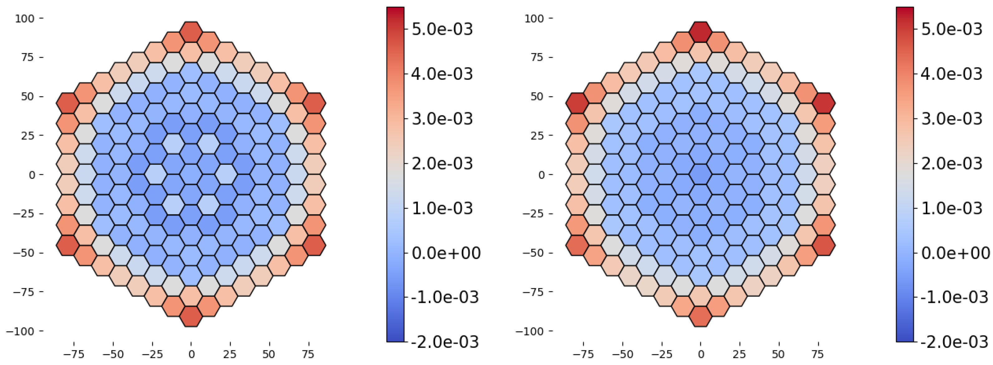
). Also, the maximum errors are of the same accuracy as the rms value, which suggests an almost flat discrepancy map, as suggested by Figure 3 for HOW, for example. The maximum discrepancies are located on the last ring of the reactor for the reflector assemblies where scattering and streaming effects are more significant. The same type of map is also observed for SNS1 or POLY.
Finally, it can be noted that the discrepancies for SNS1 deteriorate slightly from order 4 to order 5. This observation might suggest that for this benchmark case, as from k = 4 , the solution is no longer in the pre-asymptotic convergence regime with the order k. In this case, it would require h-refinement or in other terms, submeshing of the hexagon into subelements to further decrease efficiently the discrepancies. Thus, it would not be interesting to further increase the order of k for HOW and POLY to improve the accuracy for this benchmark if we maintain the hexagonal mesh only.

3.3. Numerical Results for 3D Configuration

In this part, we will now focus on the 3D case for the benchmark. The angular quadrature is a product quadrature with Gauss–Legendre for the polar angle at order 4 and Gauss–Chebyshev at order 3 for the azimuthal angle, thereby leading to 144 directions.
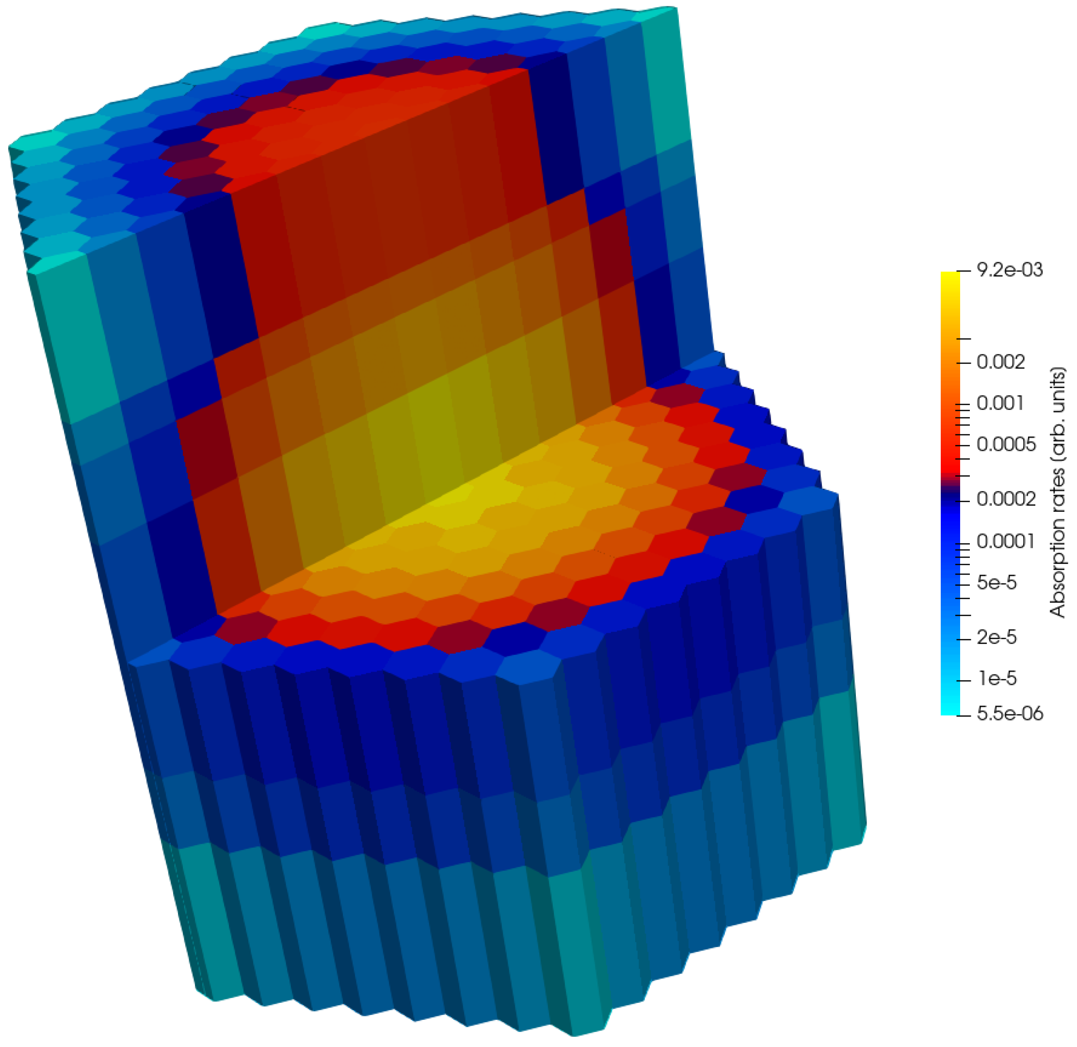
The reference solution is obtained using the same in-house solver, which refines the hexagonal cylindrical cell into parallepipeds with a lozenge base ( 3 ( lozenges ) × 4 ( radial ) × 2 ( axial ) = 24 ) and with order 5, thereby leading to 6.13 × 10 6 dofs. The reference k eff is worth 0.879836, and the reference absorption rates are computed for each hexagonal cell and are illustrated in Figure 4.
Concerning the polygonal FEM methods, we employed high-order Wachspress (HOW) and polynomial (POLY) basis functions with the multiplicative (MP) and additive (AD) extensions to 3D. No axial submeshing has been applied, and similarly, only the polynomial degree is increased to improve the modelling for axial effects. The corresponding dofs will be recalled for these solvers in the results tables.
Furthermore, we also use the solver with subdivisions of the hexagonal cylindrical cell into simply three extruded lozenges for orders 1 to 4; we denote these solutions as SNS1, which will be used to contrast the performance of the polygonal FEM schemes. The number of dofs for this case is given as ( k + 1 ) 3 . The relative stopping criteria for all iterative loops are set to 1 × 10 5 . We also recall that the total dofs N d o f s are given by N κ × N ( k ) , N κ , with similar definitions as in the 2D case.
The discrepancies on the k eff are summed up in Table 5, Table 6 and Table 7 for situations that are of interest for our analysis. On the other hand, Table 8, Table 9 and Table 10 illustrate the relative discrepancies for the absorption rates between the reference solution and the various cases for a subset of parameters, namely the types of basis functions and the associated radial, and axial degrees when relevant.

3.3.1. General Trends

The use of high-order polygonal FEM such as those developed in this work, and in particular the additive version HOW-AD and POLY-AD, leads to satisfactory results for this benchmark, especially in terms of computational cost vs. target accuracies on reactivity and local reaction rates. For instance, with POLY-AD at order 4, with five times fewer dofs than SNS1, the results are comparable both in terms of global indicators such as k eff or local values such as absorption rates.
However, it should also be noted that higher accuracies can only be achieved if the hexagonal cell is submeshed, as can be observed by the red line for k = 4 in Table 5 and Table 7, where SNS1 produces solutions with errors almost an order of magnitude lower than HOW or POLY cases. The maximum and rms discrepancies on the absorption rates confirm the same trend as in Table 8 and Table 10 for both MP and AD cases. It should be noted that, just as in the previous 2D case, the maximum errors again are located on the core periphery for reflective materials where streaming and leakage effects are exacerbated. Indeed, this benchmark problem remains quite challenging on numerical discretisation methods due to its highly heterogeneous configuration, and Takeda himself noted in [26] that some solutions obtained with an S n discretisation were not sufficient, as it required more spatial meshing.

3.3.2. Remarks on HOW/POLY MP/AD Basis Functions

For the multiplicative basis functions, the radial and axial orders may be different. From Table 6 and Table 9, for fixed k, the axial order l is varied. As l increases from 1 to 2, the results are significantly improved, e.g., for HOW-MP, Δ k e f f is reduced from 588 pcm for XY2-Z1 to 18.8 pcm for XY2-Z2, cf. the red line in Table 6 for the k eff or Table 9 for the absorption rates. However, the decrease in these discrepancies is far less, and even stagnates as l is further increased (cf. the blue lines in the same tables), and we may deduce that the errors are no longer driven by the axial effects but rather by the radial discretisation order. These results are consistent with those observed from [29], where the axial flux is approached with low-order functions. As the radial order increases from 1 to 2, HOW solutions are drastically improved compared to POLY due to more (twice) dofs.
The same conclusions hold for the AD bases, cf. Table 8, for instance, where HOW and POLY yield very comparable solutions.
Moreover, as in the 2D case, increasing the basis order is of interest until orders 3 or 4 in this benchmark, as is illustrated by Table 10 whence oscillations are observed on the precision of quantities such as the maximum error.

3.3.3. MP vs. AD: Numerical Performance

The Δ k eff values are higher with AD rather than MP cases, as can be observed from Table 5 and Table 7. Nevertheless, these differences are quite slight and very much comparable. The trend is much more favourable on the local values such as the rms discrepancies on the absorption rates, namely as from orders 3, whereby AD bases lead to more accurate results, almost twice smaller rms values, and even better considering the maximum errors. The additional dofs contained in MP bases do not contribute significantly to the accuracy of the global solution.
This numerical accuracy coupled to the fact that AD bases are composed of much fewer dofs supports the fact that these functions are very interesting for studies in reactor applications.
Table 5. Δ k e f f with respect to reference values for the 3D configuration for SNS1 and the AD cases for k [ [ 1 , 4 ] ] (cf. comments in text on coloured lines).
SNS1 ( N κ = 3549 ) HOW-AD ( N κ = 1183 ) POLY-AD ( N κ = 1183 )
k N dofs ( N ( k ) ) Δ k eff [ pcm ] N dofs ( N ( k ) ) Δ k eff [ pcm ] N dofs ( N ( k ) ) Δ k eff [ pcm ]
128,392 (8)12448281 (7)27804732 (4)3314
295,823 (27)16.422,477 (19)11411,830 (10)296
3227,136 (64)6.143,771 (37)36.423,660 (20)59.9
4443,625 (125)1.772,163 (61)−7.341,405 (35)−5.19
Table 6. Δ k e f f with respect to reference values for the 3D configuration for the MP cases with ( k , l ) [ [ 1 , 2 ] ] × [ [ 1 , 4 ] ] (cf. comments in text on coloured lines).
HOW-MP ( N κ = 1183 ) POLY-MP ( N κ = 1183 )
k , l N dofs ( N ( k ) ) Δ k eff [ pcm ] N dofs ( N ( k ) ) Δ k eff [ pcm ]
XY1-Z114,196 (12)20407098 (6)2520
XY1-Z221,294 (18)149010,647 (9)1970
XY1-Z328,392 (24)148014,196 (12)1970
XY1-Z435,490 (30)148017,745 (15)1970
XY2-Z128,392 (24)58814,196 (12)745
XY2-Z242,588 (36)18.821,294 (18)179
XY2-Z356,784 (48)14.328,392 (24)176
XY2-Z470,980 (60)13.135,490 (30)176
Table 7. Δ k e f f with respect to reference values for the 3D configuration for the MP cases with k = l [ [ 1 , 4 ] ] (cf. comments in text on coloured lines).
HOW-MP ( N κ = 1183 ) POLY-MP ( N κ = 1183 )
k , l N dofs ( N ( k ) ) Δ k eff [ pcm ] N dofs ( N ( k ) ) Δ k eff [ pcm ]
XY1-Z114,196 (12)20407098 (6)2520
XY2-Z242,588 (36)18.821,294 (18)179
XY3-Z385,176 (72)27.547,320 (40)42.9
XY4-Z4141,960 (120)−9.788,725 (75)−7.3
Table 8. Comparison of absorption rates with respect to reference values for the 3D configuration for SNS1 and the AD cases up to k = 4 (cf. comments in text on coloured lines).
SNS1HOW-ADPOLY-AD
k N dofs max [-]rms [-] N dofs max [-]rms [-] N dofs max [-]rms [-]
128,3921.8  × 10 1 6.8  × 10 2 82812.1  × 10 1 9.0  × 10 2 47323.0  × 10 1 1.2  × 10 1
295,8232.0  × 10 3 2.3  × 10 3 22,4771.2  × 10 2 1.3  × 10 2 11,8303.1  × 10 2 1.5  × 10 2
3227,1365.7  × 10 4 5.9  × 10 4 43,7712.3  × 10 3 1.8  × 10 3 23,6604.5  × 10 3 3.3  × 10 3
4443,6252.0  × 10 4 2.1  × 10 4 72,1634.3  × 10 4 8.6  × 10 4 41,4056.7  × 10 4 6.1  × 10 4
Table 9. Comparison of absorption rates with respect to reference values for the 3D configuration for the MP cases such that ( k , l ) [ [ 1 , 2 ] ] × [ [ 1 , 4 ] ] (cf. comments in text on coloured lines).
HOW-MPPOLY-MP
k , l N dofs max [-]rms [-] N dofs max [-]rms [-]
XY1-Z114,1962.1  × 10 1 7.2  × 10 2 70982.9  × 10 1 1.0  × 10 1
XY1-Z221,2946.3  × 10 2 2.7  × 10 2 10,6471.6  × 10 1 6.1  × 10 2
XY1-Z328,3926.3  × 10 2 2.7  × 10 2 14,1961.6  × 10 1 6.1  × 10 2
XY1-Z435,4906.3  × 10 2 2.7  × 10 2 17,7451.6  × 10 1 6.1  × 10 2
XY2-Z128,3921.7  × 10 1 7.1  × 10 2 14,1961.8  × 10 1 6.9  × 10 2
XY2-Z242,5881.2  × 10 2 3.2  × 10 3 21,2941.1  × 10 2 6.8  × 10 3
XY2-Z356,7841.2  × 10 2 3.1  × 10 3 28,3921.0  × 10 2 6.4  × 10 3
XY2-Z470,9801.2  × 10 2 2.9  × 10 3 35,4901.0  × 10 2 6.5  × 10 3
Table 10. Comparison of absorption rates with respect to reference values for the 3D configuration for the MP cases such that k = l [ [ 1 , 4 ] ] (cf. comments in text on coloured lines).
HOW-MPPOLY-MP
k , l N dofs max [-]rms [-] N dofs max [-]rms [-]
XY1-Z114,1962.1  × 10 1 7.2  × 10 2 70982.9  × 10 1 1.0  × 10 1
XY2-Z242,5881.2  × 10 2 3.2  × 10 3 21,2941.1  × 10 2 6.8  × 10 3
XY3-Z385,1761.1  × 10 2 3.0  × 10 3 47,3202.0  × 10 3 4.2  × 10 3
XY4-Z4141,9601.2  × 10 2 2.7  × 10 3 88,7251.0  × 10 3 1.6  × 10 3

4. Conclusions

The starting point for this work was the need to reduce computational cost-to-accuracy ratio for simulations involving neutron transport in a multiphysics setting. Indeed, we have observed that transport computations are expensive and the dominant factor for parametric studies required for reactor design or engineering studies. The target accuracy in such cases are usually around 10 pcm on reactivity and 1% for local reaction rates. Our goal in this work was to reduce the computational burden by working on the spatial discretisation for solving the neutron transport equation.
We kept the DG-FEM setting, which is usually the case for core solvers for the Apollo3® platform [30], such as Minaret [6]. Nevertheless, our main idea was to reduce the dofs by discretising the problem on the hexagon itself and avoid superfluous dofs. From past works, we have devised methods for building sets of functions that could be employed in the DG-FEM configuration [7], and we have verified their convergence properties in theoretical settings.
In this work, we have recalled the main technical points for constructing such functions and we have extended them for 3D geometries, which can be assimilated as 2D–1D meshes, or cylindrical cells with a hexagonal base. For such cases, we assumed that we already had high-order basis functions for the 2D shapes, and by combining these functions with 1D functions, we devised two types of basis functions: a full set generated as a tensor product and a set with the optimised number of functions to span the minimum space required for the solution to our problem.
We have applied these functions to solve the Takeda Model 4 benchmark in 2D and 3D. We have compared our results to a reference solution, which was highly discretised in meshing and in polynomial accuracy. Also, we have contrasted our solutions to those obtained by discretising the hexagon in three lozenges, as in [5]. Our methods yield discrepancies, which are well within the target accuracies required by studies, and with far fewer dofs, ranging from 3 to 5 in 2D and up to 10 in 3D. Although we have not compared the results in terms of computational times explicitly as these were implemented in a Python mock-up code, we can safely affirm that with all other considerations such as algorithms and iteration methods kept as before, the expected computational times will be significantly reduced.
Further works on this topic include the investigation of adaptive refining techniques to locally increase the order only where required using an error indicator as in [28]. For more challenging cases, it would also be interesting to combine the partial submeshing of some hexagonal cells in the reactor mesh with polygonal elements to improve the accuracy when required, although this should not be the case for most industrial reactor applications.

Author Contributions

Conceptualisation, D.L., A.C. and R.L.T.; methodology, D.L.; software, D.L. and A.C.; validation, D.L., A.C. and R.L.T.; investigation, D.L.; writing—original draft preparation, A.C.; writing—review and editing, A.C., R.L.T. and D.L.; visualisation, D.L. and A.C.; supervision, A.C. and R.L.T.; project administration, R.L.T.; funding acquisition, A.C. and R.L.T. All authors have read and agreed to the published version of the manuscript.

Funding

This research was funded by CEA.

Data Availability Statement

Data for the Takeda Model 4 benchmark are publicly available (https://inis.iaea.org/collection/NCLCollectionStore/_Public/22/085/22085401.pdf). The data presented in this study are available on request from the corresponding author (Source code of our implementation for the solver is not public for privacy related with the Alternative Energies and Atomic Energy Commission (CEA)).

Conflicts of Interest

The authors declare no conflicts of interest.

Appendix A. Proof of Equation (15)

Considering Legendre polynomials for V ˜ i for i [ [ 0 , k m ] ] , one should note that P ˜ i 1 span ( V ˜ i ) , so obtaining Equation (15) from Equation (14) is not straightforward.
To do so, we proceed by showing that m [ [ 0 , k ] ] , P m 2 P ˜ k m 1 j = 0 k span ( W j V ˜ k j ) .
Starting from the fact that P ˜ i 1 span ( j = 0 i V ˜ j ) , one can write that
P m 2 P ˜ k m 1 i = 0 k m P m 2 span ( V ˜ k m i )
Furthermore,
P m 2 P ˜ k m 1 i = 0 k m P m + i 2 span ( V ˜ k m i ) = j = m k P j 2 span ( V ˜ k j ) j = 0 k P j 2 span ( V ˜ k j )
Accordingly, using that P j 2 span ( W j ) , we obtain
P m 2 P ˜ k m 1 j = 0 k span ( W j ) span ( V ˜ k j ) = j = 0 k span ( W j V ˜ k j )
As this result holds m [ [ 0 , k ] ] , then going back to Equation (15), we obtain that P k 3 m = 0 k span ( W m V ˜ k m ) , as expected.
For the set of functions generating m = 0 n span ( W m 2 V ˜ n m ) to form a basis of P k 3 , the functions have to be linearly independent, which is achieved if span ( m = 0 k W m V ˜ k m ) = { 0 } . This is the case, as we have previously opted for V l to be the Legendre polynomials, which are orthogonal, and W k , forming a basis for the regular hexagons; by definition, its elements are linearly independent. Accordingly, Equation (15) is verified.

References

  1. Cattaneo, P.; Lenain, R.; Merle, E.; Patricot, C.; Schneider, D. Numerical optimization of a multiphysics calculation scheme based on partial convergence. Ann. Nucl. Energy 2021, 151, 107892. [Google Scholar] [CrossRef]
  2. Delvaux, R.; Patricot, C. Application of the Adaptive Residual Balance Method on an APOLLO3®-THEDI Coupling and Comparison with Anderson Acceleration. In Proceedings of the International Conference on Mathematics and Computational Methods Applied to Nuclear Science and Engineering-M and C, Virtual Meeting, 3–7 October 2021. [Google Scholar]
  3. Zhang, H.; Guo, J.; Lu, J.; Li, F.; Xu, Y.; Downar, T.J. An Assessment of Coupling Algorithms in HTR Simulator TINTE. Nucl. Sci. Eng. 2018, 190, 287–309. [Google Scholar] [CrossRef]
  4. Guyot, M. Neutronics and Thermal-Hydraulics Coupling: Some Contributions toward an Improved Methodology to Simulate the Initiating Phase of a Severe Accident in a Sodium Fast Reactor; Technical Report; Universite d’Aix-Marseille: Marseille, France, 2014. [Google Scholar]
  5. Gastaldo, L.; Le Tellier, R.; Suteau, C.; Fournier, D.; Ruggieri, J.M. High-order discrete ordinate transport in non-conforming 2D Cartesian meshes. In Proceedings of the International Conference on Mathematics, Computational Methods & Reactor Physics, New York, NY, USA, 3–7 May 2009. [Google Scholar]
  6. Lautard, J.J.; Moller, J.Y. MINARET, a deterministic neutron transport solver for nuclear core calculations. In Proceedings of the International Conference on Mathematics, Computational Methods & Reactor Physics, M&C, Rio de Janeiro, Brazil, 8–12 May 2011. [Google Scholar]
  7. Labeurthre, D.; Calloo, A.; Le Tellier, R. High-order Wachspress functions on convex polygons through computer algebra. J. Comput. Phys. 2022, 470, 111545. [Google Scholar] [CrossRef]
  8. Chandrasekhar, S. Radiative Transfer; Oxford University Press: Oxford, UK, 1950. [Google Scholar]
  9. Carlson, B.G. Solution of the Transport Equation by Sn Approximations; Technical Report; Los Alamos Scientific Laboratory: Los Alamos, NM, USA, 1953. [Google Scholar]
  10. Reed, W.H.; Hill, T.R. Triangular Mesh Methods for the Neutron Transport Equation; Technical Report; Los Alamos Scientific Laboratory: Los Alamos, NM, USA, 1973. [Google Scholar]
  11. Hébert, A. Applied Reactor Physics; Presses Internationales Polytechnique: Montréal, QC, Canada, 2009. [Google Scholar]
  12. Wachspress, E.L. A Rational Finite Element Basis; Academic Press: Cambridge, MA, USA, 1975. [Google Scholar]
  13. Floater, M.S. Generalized barycentric coordinates and applications. Acta Numer. 2015, 24, 161–214. [Google Scholar] [CrossRef]
  14. Sukumar, N. Construction of polygonal interpolants: A maximum entropy approach. Int. J. Numer. Methods Eng. 2004, 61, 2159–2181. [Google Scholar] [CrossRef]
  15. Hormann, K.; Sukumar, N. Maximum entropy coordinates for arbitrary polytopes. In Computer Graphics Forum; Wiley Online Library: Hoboken, NJ, USA, 2008; Volume 27, pp. 1513–1520. [Google Scholar]
  16. Gout, J.L. Rational Wachspress-type Finite Elements on Regular Hexagons. IMA J. Numer. Anal. 1985, 5, 59–77. [Google Scholar] [CrossRef]
  17. Jaśkowiec, J. Very high order discontinuous Galerkin method in elliptic problems. Comput. Mech. 2018, 62, 1–21. [Google Scholar] [CrossRef]
  18. Jaśkowiec, J.; Pluciński, P.; Stankiewicz, A. Discontinuous Galerkin method with arbitrary polygonal finite elements. Finite Elem. Anal. Des. 2016, 120, 1–17. [Google Scholar] [CrossRef]
  19. Bourhrara, L. A new numerical method for solving the Boltzmann transport equation using the Pn method and the discontinuous finite elements on unstructured and curved meshes. J. Comput. Phys. 2019, 397, 108801. [Google Scholar] [CrossRef]
  20. Gout, J.L. Éléments Finis Polygonaux de Wachspress. Ph.D. Thesis, Université de Pau, Pau, France, 1980. [Google Scholar]
  21. Calloo, A.; Le Tellier, R.; Labeurthre, D. High-order finite elements for the neutron transport equation on honeycomb meshes. In Proceedings of the EPJ Web of Conferences, EDP Sciences, Cambridge, UK, 29 March–2 April 2020; Volume 247, p. 3002. [Google Scholar]
  22. Labeurthre, D.; Calloo, A.; Le Tellier, R. Verification and Comparison of Finite Element Bases for an Upwind Discontinuous Galerkin Discretization of the Transport Equation on Honeycomb Meshes. In Proceedings of the Mathematics & Computation (M&C) 2023, Niagara Falls, ON, Canada, 13–17 August 2023. [Google Scholar]
  23. Hébert, A. A Raviart-Thomas-Schneider implementation of the simplified Pn method in 3-D hexagonal geometry. In Proceedings of the International Conference on the Physics of Reactor, (PHYSOR), Pittsburgh, PA, USA, 9–14 May 2010; American Nuclear Society: Pittsburgh, PA, USA, 2010. [Google Scholar]
  24. Richter, G.R. An optimal-order error estimate for the discontinuous Galerkin method. Math. Comput. 1988, 50, 75–88. [Google Scholar] [CrossRef]
  25. Mukherjee, T. Hierarchical Polygonal Finite Elements of Arbitrary Order. Ph.D. Thesis, McGill University, Montreal, QC, Canada, 2015. [Google Scholar]
  26. Takeda, T.; Ikeda, H. 3-D neutron transport benchmarks. J. Nucl. Sci. Technol. 1991, 28, 656–669. [Google Scholar] [CrossRef]
  27. Johnson, C.; Pitkäranta, J. Convergence of a fully discrete scheme for two-dimensional neutron transport. SIAM J. Numer. Anal. 1983, 20, 951–966. [Google Scholar] [CrossRef]
  28. Fournier, D.; Herbin, R.; Tellier, R.L. Discontinuous Galerkin Discretization and hp-Refinement for the Resolution of the Neutron Transport Equation. SIAM J. Sci. Comput. 2013, 35, A936–A956. [Google Scholar] [CrossRef]
  29. Collins, B.; Stimpson, S.; Kelley, B.W.; Young, M.T.; Kochunas, B.; Graham, A.; Larsen, E.W.; Downar, T.; Godfrey, A. Stability and accuracy of 3D neutron transport simulations using the 2D/1D method in MPACT. J. Comput. Phys. 2016, 326, 612–628. [Google Scholar] [CrossRef]
  30. Mosca, P.; Bourhrara, L.; Calloo, A.; Gammicchia, A.; Goubioud, F.; Mao, L.; Madiot, F.; Malouch, F.; Masiello, E.; Moreau, F.; et al. APOLLO3®: Overview of the new Code Capabilities for Reactor Physics Analysis. In Proceedings of the Mathematics & Computation (M&C) 2023, Niagara Falls, ON, Canada, 13–17 August 2023. [Google Scholar]
Figure 1. Geometrical elements to define Wachspress shape functions on a regular hexagon (in green) defined with vertices in blue dots at p = 3 . Adapted from [7].
Jne 05 00006 g001
Figure 2. Radial plane from the Takeda Model 4 benchmark adapted from [26].
Jne 05 00006 g002
Figure 3. Discrepancy distribution on the absorption rates for the HOW case at k = 3 (left) and k = 5 (right), Units = [-].
Jne 05 00006 g003
Figure 4. Reference absorption rates distribution, integrated in each spatial cell in the 3D mesh.
Jne 05 00006 g004
Table 1. Number of dofs for each of the four 3D bases.
WachspressPolynomial
OrderMultiplicativeAdditiveMultiplicativeAdditive
112764
236191810
372374020
4120617535
51809112656
Table 2. Material indices in each axial plane along the diagonal AA’ described in Figure 2 for the Takeda core.
Height (cm)Material Indices along AA’
Central Hexagon
19010987111111178910
155
145
14510987332223378910
125
12510987654445678910
95
65
6510987332223378910
45
4510987111111178910
0
1: Steel; 2: Axial blanket; 3: Axial Reflector; 4: Test zone; 5: Driver zone with moderator; 6: Driver zone w/o moderator; 7: Reflector w/o moderator; 8: Reflector with moderator; 9: KNK-1 Reflector; 10: Sodium/Steel zone.
Table 3. Δ k e f f with respect to reference value for the 2D configuration (cf. comments in text on coloured lines).
SNS1 ( N κ = 507 ) HOW ( N κ = 169 ) POLY ( N κ = 169 )
k N dofs ( N ( k ) ) Δ k eff [ pcm ] N dofs ( N ( k ) ) Δ k eff [ pcm ] N dofs ( N ( k ) ) Δ k eff [ pcm ]
12028 (4) 779.5 1024 (6)1721.2507 (3)−2277
24563 (9)13.02028 (12)−16.61024 (6)199.6
38112 (16)4.73042 (18)32.51690 (10)9.8
412,675 (25)−0.44056 (24)−11.12535 (15)−2.3
518,252 (36)−0.55070 (30)5.13549 (21)−0.1
Table 4. Comparison of absorption rates with respect to reference values for the 2D configuration (cf. comments in text on coloured lines).
SNS1HOWPOLY
k N dofs Max [-]rms [-] N dofs Max [-]rms [-] N dofs max [-]rms [-]
120283.0  × 10 2 1.4  × 10 2 10246.2  × 10 2 3.1  × 10 2 5071.5  × 10 1 7.5  × 10 2
245636.6  × 10 4 5.7  × 10 4 20282.1  × 10 3 9.7  × 10 4 10241.1  × 10 2 5.5  × 10 3
381122   × 10 4 1.6  × 10 4 30423.8  × 10 3 1.4  × 10 3 16902.3  × 10 3 3.4  × 10 3
412,6754.3  × 10 5 2.4  × 10 5 40563.4  × 10 3 1.3  × 10 3 25357.6  × 10 4 6.5  × 10 4
518,2529.1  × 10 5 3.5  × 10 5 50705.3  × 10 3 1.8  × 10 3 35498.8  × 10 4 2.4  × 10 4
Disclaimer/Publisher’s Note: The statements, opinions and data contained in all publications are solely those of the individual author(s) and contributor(s) and not of MDPI and/or the editor(s). MDPI and/or the editor(s) disclaim responsibility for any injury to people or property resulting from any ideas, methods, instructions or products referred to in the content.

