An Innovative PEMFC Magnetic Field Emulator to Validate the Ability of a Magnetic Field Analyzer to Detect 3D Faults

Abstract

An original non-invasive methodology of the fuel cell diagnosis is proposed to identify different positions of the faults in Proton Exchange Membrane Fuel Cell (PEMFC) stacks from external magnetic field measurements. The approach is based on computing the external magnetic field difference between normal and faulty PEMFC operating conditions. To evaluate the external magnetic field distribution, in this paper, we propose an improved design of the magnetic field analyzer. This analyzer amplifies the magnetic field around the cell to perform an accurate detection of the fault position. Moreover, the main contribution of this work is represented by conceiving and implementing a 3D multi-physical current distribution emulator of a proton exchange membrane fuel cell. The new concept of a proton exchange membrane fuel cell emulator has been specially designed to emulate the magnetic field of a real fuel cell stack. This emulator concept is also beneficial for a new model of the fuel cell, which implies a multi-physical coupling between electrochemical electric conduction and the generated magnetic field. Finally, finally, the numerical model and the emulator have been involved in the realization of numerical simulations and experimental analysis to prove the ability of the system to detect and localize 3D faults.

1. Introduction

The Fuel Cell (FC) technology has been known since 1839 [1], but it was not commercially used until the space race began in the late 1950s. Since the late 1990s, the scientific research on the FC has increased [2,3,4,5] and recently, many companies have started to commercialize this technology which is well adapted for different vehicular applications [6,7] particularly when hydrogen is produced with non-fossil energy resources [8]. Up to now, the durability, reliability, and efficiency [9,10,11,12,13,14] are still significant issues under continuous studies to achieve the most effective system. Diagnosis of FC is an important issue, which allows identifying faults operations [15,16] to reduce repair time [17] and, therefore, possibly increase the FC lifetime. Earlier works proposed physical model based diagnostic [18,19,20,21,22] or data based diagnostic [23,24,25,26] which will help FCs deployment. Knowing the fault position inside the FC stack can indicate the cause of the fault [27], as well as identify the faulty cell inside the stack. Electrochemical Impedance Spectroscopy (EIS) [28,29,30,31,32,33,34] can be used for diagnosis but does not allow to know the local distribution of the current. As the local current density distribution is linked directly to the ionic flow inside the electrolyte of an FC, assessing it can give important information about FC state-of-health [35]. Assessing the local current is not directly possible from the global current measurement. The local current evaluation needs some sophisticated methods that can be divided into two main categories: invasive and non-invasive techniques. In the first category, several techniques have studied Proton Exchange Membrane Fuel Cell (PEMFC) behavior through direct and indirect local current density measurement methods. The direct approach is characterized by segmented [36] and non-segmented [37] Bipolar Plate (BP) with a printed circuit board (PCB) current measurement technology [38]. In addition to these methods, sensors can be inserted into the rib of the cathode separator [39] to measure the current distribution directly. Reversely, indirect methods can be based on the measurement of the magnetic field inside PEMFC to compute the current density using Maxwell’s equations. In [40], the magnetic sensors were located inside each boring created at the level of the conductive plate, while in [41], the sensors were embedded inside the cooling holes of PEMFC. Furthermore, reference [42] presents an integrated plate with vertical and horizontal holes to measure the magnetic field inside the volume of the FC stack. In addition to the invasive methods, reference [43] shows the S++ technology, which uses a current scan line device placed between the halves of the BP at an arbitrary place in the stack to measure the current density distribution in a large FC stack. The latter, even if it can lead directly to the measurement of the local current distribution, still suffers from the direct effect of these inserted sensors on the current distribution inside the stack, making it hard to know if the fault is due to the diagnosis setup or the stack itself. On the contrary, magneto-tomography technology is based on an external magnetic field measurement by using magnetic sensors located around the FC without affecting the stack behavior [44]. This is done by measuring 100 points using a tri-axial magnetic sensor moving around the stack via a robot arm to get a good resolution for the current mapping. The main obstacle to using this method is the time taken by the acquisition and calculation (around 15 min). During this time, the current behavior inside the stack will change, leading to non-accurate measurements. More recent work in [45] proposed a method to detect and isolate the fault by monitoring the current distribution with the aid of the external magnetic field without using the inverse problem. Furthermore, references [46,47] presents an acquisition time reduction for the current density and calculation to 1 min by using 30 magnetic sensors, all fixed around the stack. This work suffers from inaccurate fault detection and detects only the general faults which affect the whole stack uniformly. More advanced work in [48,49] covers the local fault by proposing a 3D fault identification method. Moreover, the external magnetic field measurements are dedicated to other diagnosis methods, like data-driven diagnosis strategies in fault identification and classification at various levels [50,51]. Other non-invasive methods such as neutron imaging [52] can examine the water distribution inside the FC by giving indirect information about the current density inside the stack.

Recent work realized in our research team proposed an innovative magnetic field analyzer that amplifies the measured magnetic field by using a specially designed ferromagnetic circuit [53]. This analyzer has been applied on a 2D FC emulator composed of 16 aluminum bars insulated from each other, thereby allowing to set the current density to flow inside each bar. This has been done to emulate the current density in a cutting plane within a stack. For a 2D default, this methodology shows higher magnetic field differences $\Delta B=B_{normal}-B_{fault}$ between normal and faulty operation due to the high permeability of the material used.

The purpose of this work is to improve non-invasive diagnostic methodologies based on the FC external magnetic field measurement. Before considering the evaluation of the proposed diagnosis methodology on actual fuel cell stacks, generating a similar current distribution inside an FC emulator with similar geometry and structure is helpful for designing both numerical modeling and experimental magnetic field measurements.

The main contribution of this work is represented by an innovative 3D current density emulator of a PEMFC. Based on a passivized FC structure, supplied by a current source, this emulator reproduces an equivalent current distribution in a similar geometrical domain, as the current distribution inside a Fuel Cell domain, during steady state operation.

For the numerical simulation, a numerical model, computing the magnetic field produced during FC operation includes the emulator concept in the following coupling strategy: an FC Multi physical model involving couplings between electrochemical and electric conduction is used to specify the dependency between the current density and the electric field inside emulator regions, to reproduce similar current distribution. The magnetic field generated by the current distribution in the emulator will also reproduce the magnetic field of the real FC. This emulator concept simplifies the numerical analysis of the magnetic field produced by the FC, as it implies easier coupling between electric conduction and magnetic equations by using the 3D Finite Element Method. Then an updated design for the magnetic field analyzer and the methodology were validated for realistic 3D local faults inside the FC stack emulator. For normal and faulty operation of the fuel cell, the results of the magnetic field numerical simulation are compared with the experimental magnetic field measurements obtained with the magnetic field analyzer positioned around the FC emulator.

Finally, the numerical model and the emulator have been involved in the realization of numerical simulations and experimental analysis to prove the ability of the system to detect and localize 3D faults.

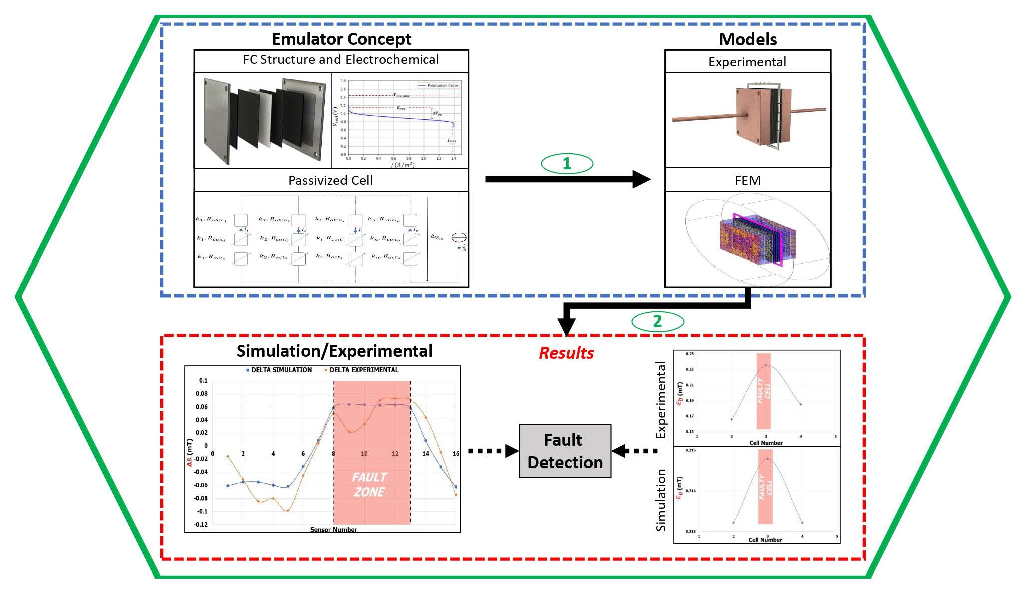
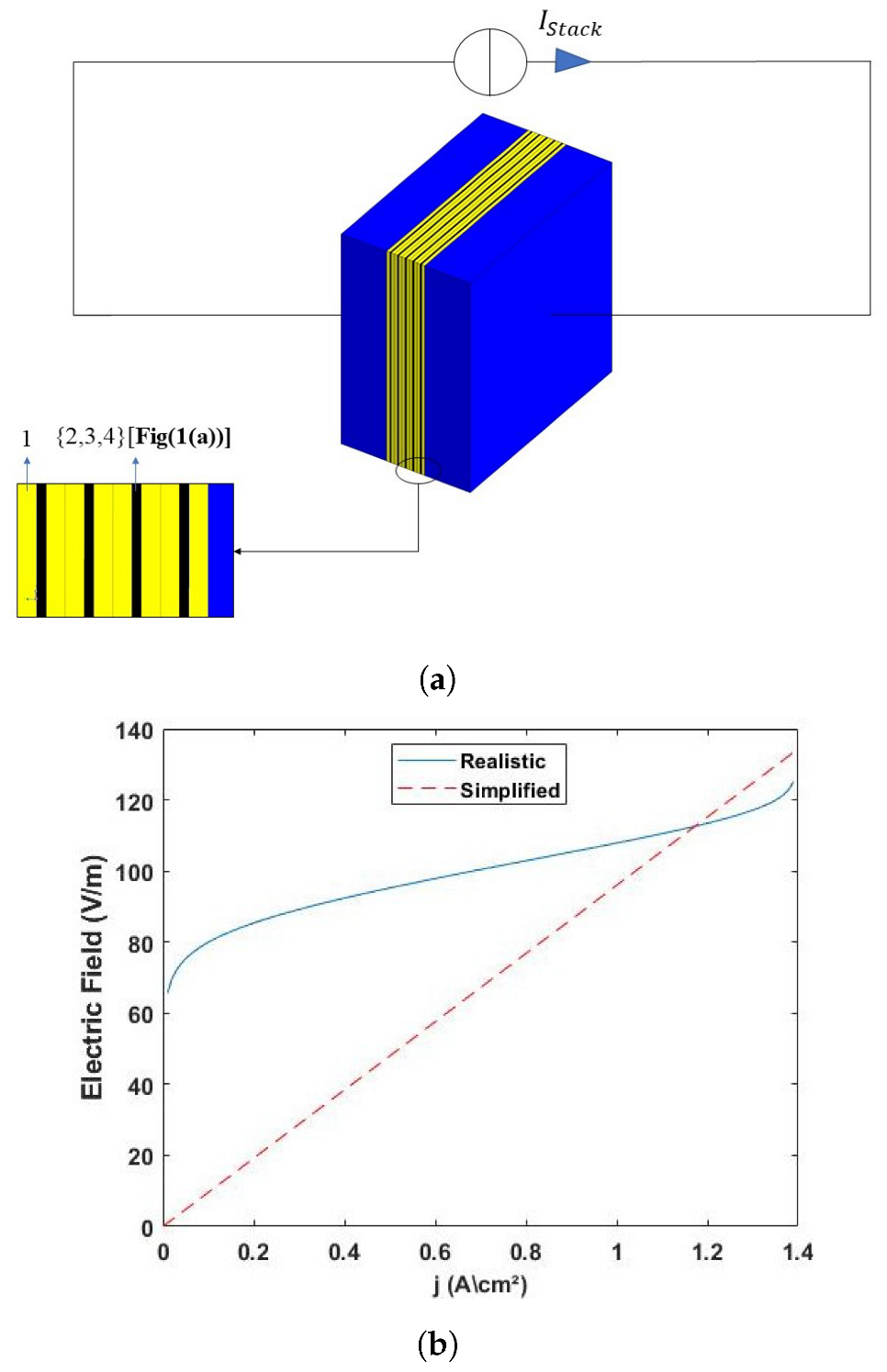
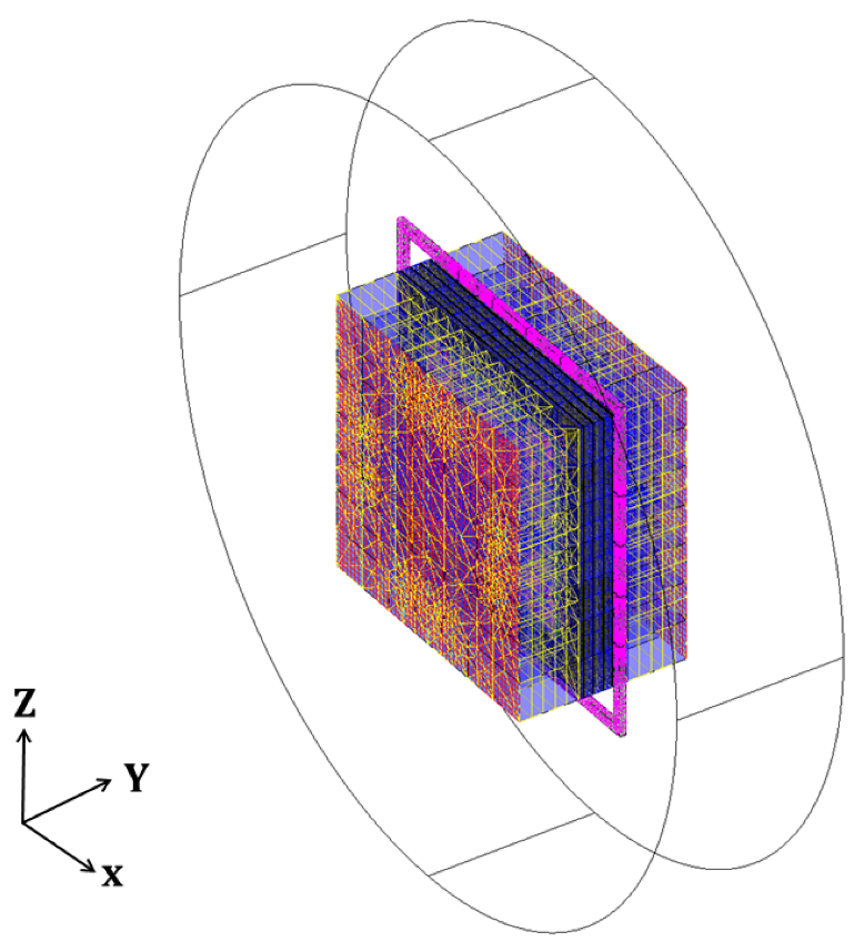
2. 3D PEMFC Current Density Emulator

This emulator is based on a multi-physics coupling between electrochemical, electrical, and magnetic models of the PEMFC stack. These couplings produce homogeneous and heterogeneous current flows according to the operating conditions of the cell. This emulator demonstrates these distributions in the static state of the PEMFC, without considering the startup and shutdown of the cell.

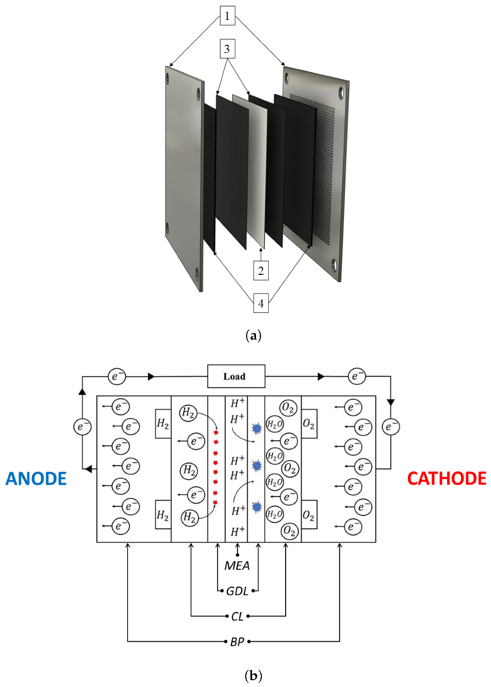
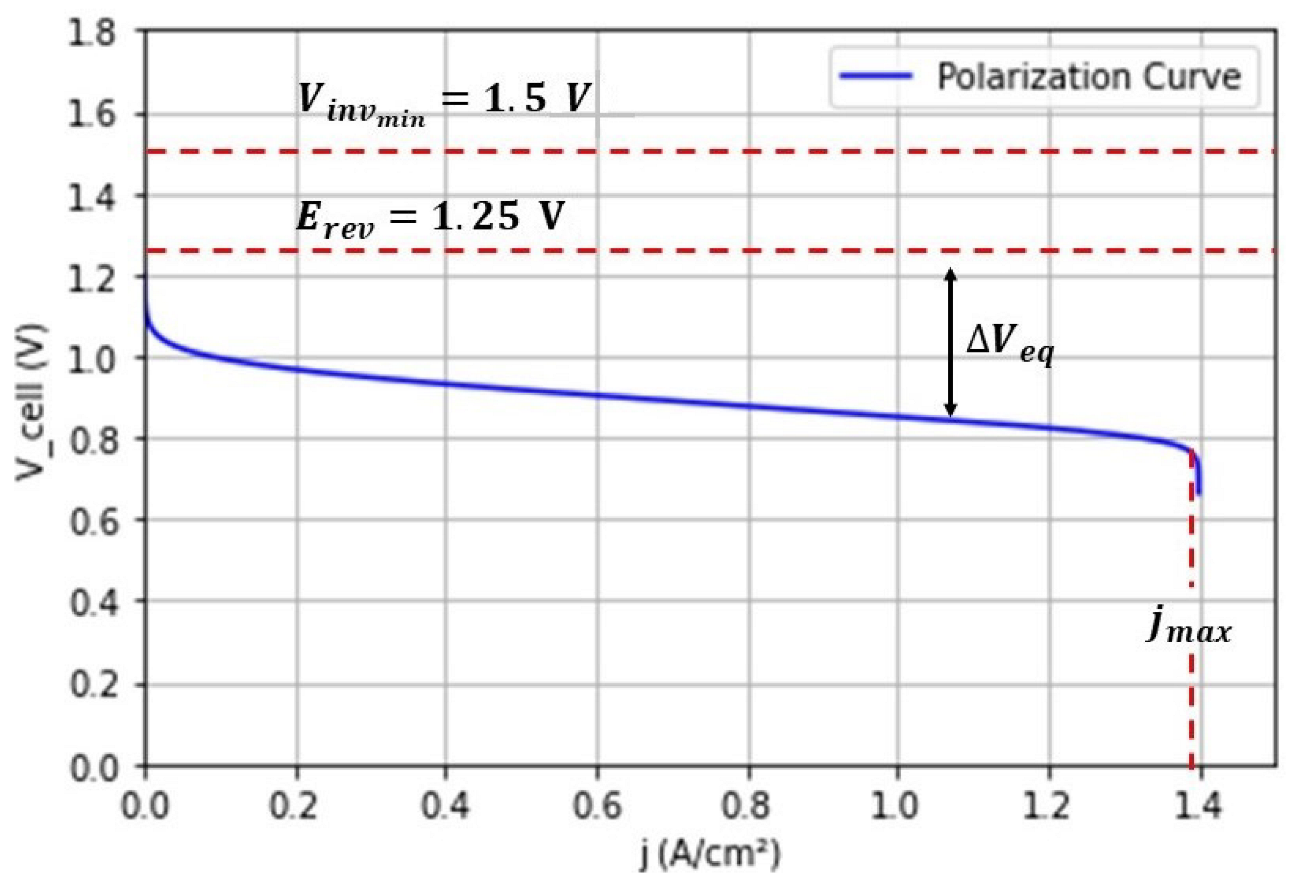
2.1. FC Structure and Electrochemical Consideration

A hydrogen fuel cell generates electrical energy from a redox reaction between hydrogen and oxygen. In the case of a PEMFC (Proton Exchange Membrane Fuel Cell), the electrolyte is a solid polymer allowing the protons mobility. The structure of a PEM single cell is shown in Figure 1a: the anode and cathode bipolar plates (BP) (1) are separated by a membrane electrolyte assembly (MEA). The MEA is structured in five layers: the polymer electrolyte membrane (2), two thin conductive catalyst/electrode layers in direct contact with each side of the electrolyte membrane (3), and two porous conductive gas diffusion layers (GDL) ensuring the distribution of gas reactants at the catalyst/electrode level (4). The GDL also forms an electrical connection between the electrodes and the bipolar plates [54]. The Bipolar plate design includes gas channels to supply gas reactants at the anode and cathode sides. As shown in Figure 1b, the hydrogen is oxidized at the anode electrode and releases $H^{+}$ ions that migrate through the electrolyte membrane. At the cathode, the oxygen is reduced and combines with $H^{+}$ ions forming water. Water is, therefore, a by-product of the redox reaction. Besides electrical energy, it is worth mentioning that thermal power is also generated by this exothermic reaction.

In an FC stack, multiple single cells are packed in series, to increase the global voltage. The FC stack is bounded by two conductive plates also used to connect the FC stack with the external electric circuit.

At the level of every single cell, an electrochemical model provides the relationship between the voltage and the global current density at the cell membrane level, $V=f\left(j\right)$. This relationship can lead to the representation of a polarization curve as shown in Figure 2, which depends on many physical parameters like pressure, temperature, gas stoichiometry, and humidity. This voltage-current density dependency is explained by Equation (1) in the literature [55].

$$v\left(j\right)=E_{rev}-v_{act}-v_{ohm}-v_{con}$$

(1)

In Equation (1), $E_{rev}$ represents the reversible voltage given by the Nernst equation, depending on cell temperature and on the reactant’s partial pressures, $v_{act}$ the activation drop voltage caused by slow reaction at the electrode surface level [55], usually approximated by Tafel equation Equation (2).

$$v_{act}=\frac{RT}{2F\alpha }ln(\frac{j}{j_0})$$

(2)

where $\alpha$ is the charge transfer coefficient, R is the universal gas constant, T is the cell temperature, $j_0$ is the exchange current density at which the overvoltage begins to move from zero, and F is the Faraday constant.

$v_{ohmic}$, the ohmic voltage drop can be expressed in Equation (3) where ${\rho }_m$ is the specific ionic resistivity of the membrane, ${\rho }_{GDL}$ the GDL resistivity, $t_m$ and $t_{GDL}$ represent the membrane and the GDL thickness.

$$v_{ohmic}=j(t_m.{\rho }_m+2.t_{GDL}.{\rho }_{GDL})$$

(3)

$v_{con}$, the concentration voltage drop of Equation (4) in [55], which results from the reduction of the concentration of the reactants on the electrodes. The influence of $v_{con}$ can be observed in Figure 2 when the current density j is close to the maximum value $j_{max}$, thereby causing a failure in the transport of enough reactant to the electrode surface.

$$v_{con}=\frac{RT}{2F\alpha }\ln (1-\frac{j}{j_{max}})$$

(4)

Inside the FC, at the level of the MEA, the current flow is ensured by the electrons flow at the level of the conductive GDL and by the hydrogen ions flow inside the membrane electrolyte. Electron-ion exchange occurs at the electrodes (catalyst layers) level. The electrolyte membrane, coated by electrodes, is covered by a GDL on both sides, as shown in Figure 1a.

If ${\rho }_{GDL}$ can be considered constant, the ionic resistivity of the membrane ${\rho }_m$ depends on the current density, temperature, and membrane hydration. In Figure 2, the dependence $V=f\left(j\right)$ has been obtained from Equation (1) to Equation (4) using the parameters presented in

Table 1. Main parameters for the polarization curve [56].

${\mathit{E}}_{\mathit{rev}}$ (V)	${\mathit{j}}_{\mathit{max}}\left(\raisebox{1ex}{$\mathbf{A}$}\!\left/ \!\raisebox{-1ex}{${\mathbf{cm}}^2$}\right.\right)$	${\mathit{j}}_0\left(\raisebox{1ex}{$\mathbf{A}$}\!\left/ \!\raisebox{-1ex}{${\mathbf{cm}}^2$}\right.\right)$	$\mathit{T}{(}^{\circ }\mathbf{C})$	$\mathit{\alpha }$
1.25	1.4	$8.8\times {10}^{-8}$	60	0.5

and which is given by experimental study presented in [56].

Another electrochemical aspect considered in this analysis consists in the impossibility of an inverse current density at the level of the electrolyte membrane in steady-state operation of the FC, even for a fault zone of the electrolyte membrane producing a lower reversible voltage than the overall cell voltage. As shown in Figure 2, a reverse current in the electrolyte assumes a voltage between the electrodes of the cell, $V_{in{v}_{min}}$, exceeding the activation losses in addition to the reversible voltage, which is not possible. For example, in the conditions mentioned in Table 1, even for a very low current density value $V_{in{v}_{min}}=1.5$ V.

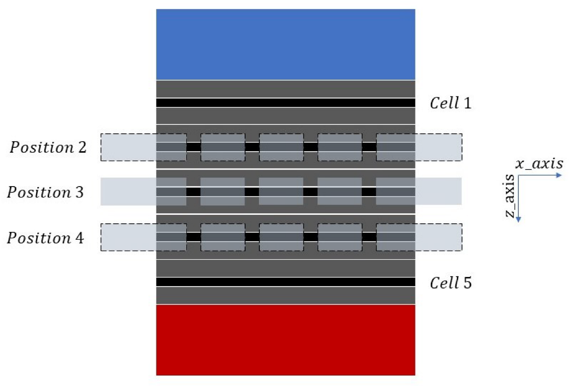
2.2. Current Density Distribution inside the Real FC and the Proposed Emulator

The final aim of this work would be to be able to diagnose a sampled selection of fuel cell stacks coming out of a production line, reducing, therefore, time-to-market times for fuel cell manufacturers. Before considering the evaluation of the proposed diagnosis methodology on actual fuel cell stacks, generating a similar current distribution inside an FC emulator with similar geometry and structure is beneficial for designing both numerical modeling and experimental magnetic field measurements. The experimental cost is reduced, as the current density of the FC is based on a passivized device supplied by an external current source. For the numerical modeling, this implies easier coupling between electric and magnetostatic problems using the 3D Finite Element Method (FEM) with Altair Flux environment [57].

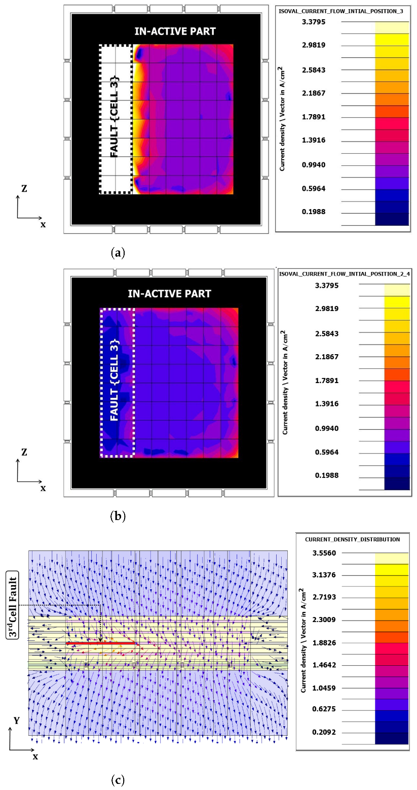
2.2.1. Current Density Distribution inside the FC

Due to the physical parameter’s variation while the stacking operation, a fault can occur. In [58], both 2D and 3D faults were introduced, where the 3D faults are the sum of the 2D faults by taking into consideration each component inside the FC to build the current basis. As mentioned previously, the FC local current density cannot be negative. Even though there is a significant voltage difference between the normal and fault areas in the cell, reverse current conduction is not possible.

In Figure 3a, we consider a discretization of one cell electrolyte surface in n elements, and the discretized current distribution corresponding to the set of n surface elements. For each surface element i, an equivalent circuit, see Figure 3b corresponding to Equation (1) as associated in series with a linear resistor and two non-linear resistors, is used to model the voltage drops. As only a positive current density is possible at the electrolyte membrane level, for each surface element, a diode was also added in the MEA equivalent electric circuit.

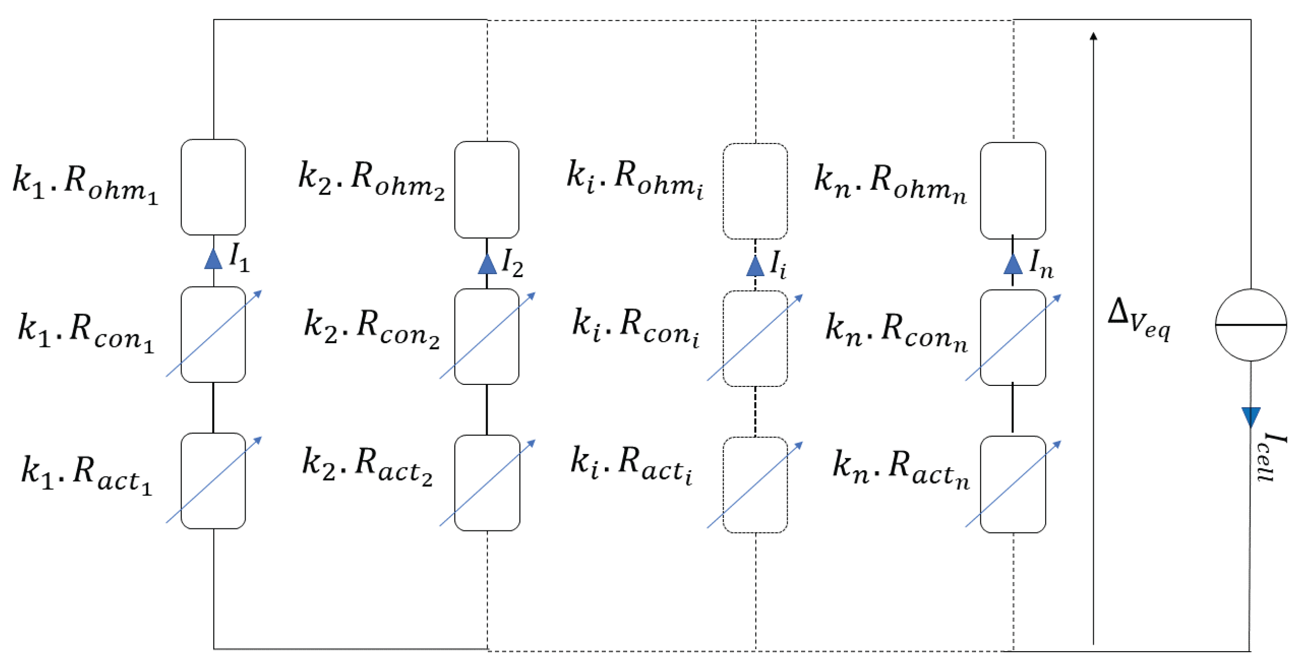
2.2.2. A FC Emulator Concept

Due to the high membrane conductivity of an FC, the Passivized Cell (PC) is modeled by an anode and cathode BP separated by two GDLs instead of MEA represented in Figure 1a. To analyze the current for n surface elements of the FC, we can observe two situations in Figure 3b circuit:

• If $E_{re{v}_i}<V_{cell}$ then $I_i=0$ which can be equivalent with a very high resistivity of $R_{e{q}_i}=R_{ac{t}_i}+R_{oh{m}_i}+R_{co{n}_i}$
• If $E_{re{v}_i}>V_{cell}$ then $I_i>0$

As the currents $I_1,I_2,\dots ,I_n$ have the same direction, identical values can be obtained in the FC equivalent circuit presented in Figure 4 and the passivized cell model given in Figure 3b.

This model keeps resistive components multiplied by corrective constants $k_1,k_2,\dots ,k_n$. These factors can be obtained using the FC circuit and the passivized circuit. Therefore, the current in the FC circuit of Figure 3b can be expressed by

$$I_i=\{\begin{array}{cc}\frac{E_{re{v}_i}-V_{cell}}{R_{ac{t}_i}+R_{co{n}_i}+R_{oh{m}_i}},& \mathrm{if}{E}_{re{v}_i}>V_{cell}\\ 0,\hfill & \mathrm{if}{E}_{re{v}_i}\le V_{cell}\end{array}$$

Identical current values can be obtained in the passivized FC emulator Figure 4 circuit after exprsing the corrective constant $k_i$ by

$$k_i=\{\begin{array}{cc}\frac{\Delta V_{eq\left(normal\right)}}{E_{re{v}_i}-V_{cell}},& \mathrm{if}{E}_{re{v}_i}>V_{cell}\\ \infty ,\hfill & \mathrm{if}{E}_{re{v}_i}<V_{cell}\end{array}$$

where $\Delta V_{eq\left(normal\right)}$ is the supplying voltage source that can be considered by the difference between the cell reversible voltage and the considered value of the cell given in Equation (5) when Temperature (T) and Pressure (P) are considered at a homogeneous value for the part of the cell in normal operation.

$$\Delta V_{eq}\left(J\right)=E_{rev}(T,P)-V_{cell}\left(J\right)$$

(5)

Creating a simplified current density distribution, similar to that inside the actual FC, makes it easier to study the magnetic field generated by the Passivized Cell (PC), and implicitly by the FC operation.

2.2.3. Electric Conduction Problem of the Passivized FC

To analyze the current density inside the FC, an electric conduction FEM model supplied by a current source has been implemented as shown in Figure 5a. In this model, the geometry and the structure of a passivized FC have been used. The physical properties, such as the resistivity of the BP and End Plates (EP), are the same as for the FC materials. Two approaches have been used to analyze the current density distribution inside the FC emulator: a realistic FC behavior, and a simplified FC behavior.

A realistic behavior was obtained by using the electric field characteristics at the membrane level. The $E\left(j\right)$ is computed based on Equation (6), where $\Delta V_{eq}\left(j\right)$ characteristics is given by Equation (5) to obtain the non-linear active area behavior represented in Figure 5b where $d_{mem}$ [56] is the membrane thickness.

$$E\left(j\right)=\frac{\Delta V_{eq}\left(j\right)}{d_{mem}}$$

(6)

In the simplified approach, a linearized $E\left(j\right)$ was considered by the means of an average resistivity MEA presented in [56] as shown in Figure 5b.

In this paper, the simplified model is explained by the $PC$ structure, where the active area is considered by only two GDLs. This GDL resistivity has been computed depending on an experimental test done which measures $\Delta V_{normal}$ between two BP after supplying our emulator with $70A$ to calculate after that ${\rho }_{GDL}$ using ohms law and Equation (7), respectively.

$$R={\rho }_{GDL}\frac{t_{GDL}}{A_{GDL}}$$

(7)

where $t_{GDL}$ is the GDL thickness and $A_{GDL}$ is the surface area of the GDL.

Table 2. Features of the FC stack emulator and ferromagnetic analyzer.

Plates	Materials	Resistivity $(\Omega .\mathbf{m})$	${\mathit{\mu }}_{\mathit{r}}$	Dimension (mm2)	Thickness (mm)
End plate	Aluminium	$2.65\times {10}^{-8}$	1	$140\times 140$	30
Bipolar Plate	Graphite	$3\times {10}^{-5}$	1	$140\times 140$	2
		Normal :
GDL	Carbon cloth	$6.0571\times {10}^{-3}$	1	$100\times 100$	0.5
		Fault: Insulator Infinite
Ferromagnetic	Ni-Fe Family	___	741	$160\times 160$	3

represents the main physical and geometric features of the emulator as well as of the ferromagnetic circuit analyzer.

In both realistic and simplified approaches, the $E\left(j\right)$ behavior is considered homogeneous for the part of the cell in normal operation, as physical parameters like Temperature (T), Pressure (P), humidity, and stoichiometry are considered constant over the active surface.

3. Experimental and Numerical Modeling Results

To prove the effectiveness of the simplified approach, the next paragraph will analyze and compare the numerical with the experimental results of this approach. In both findings, the fabricated ${\Delta }_B$ by the magnetic sensors was computed at different circuit analyzer positions around a 5-cell stack emulator. These positions were localized around Cell 2, Cell 3 (faulty cell), and Cell 4, see Figure 6.

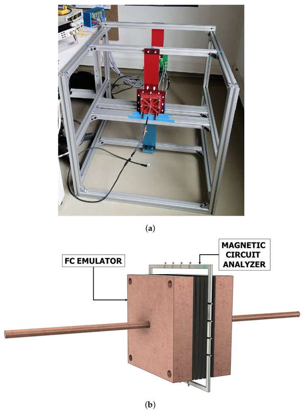
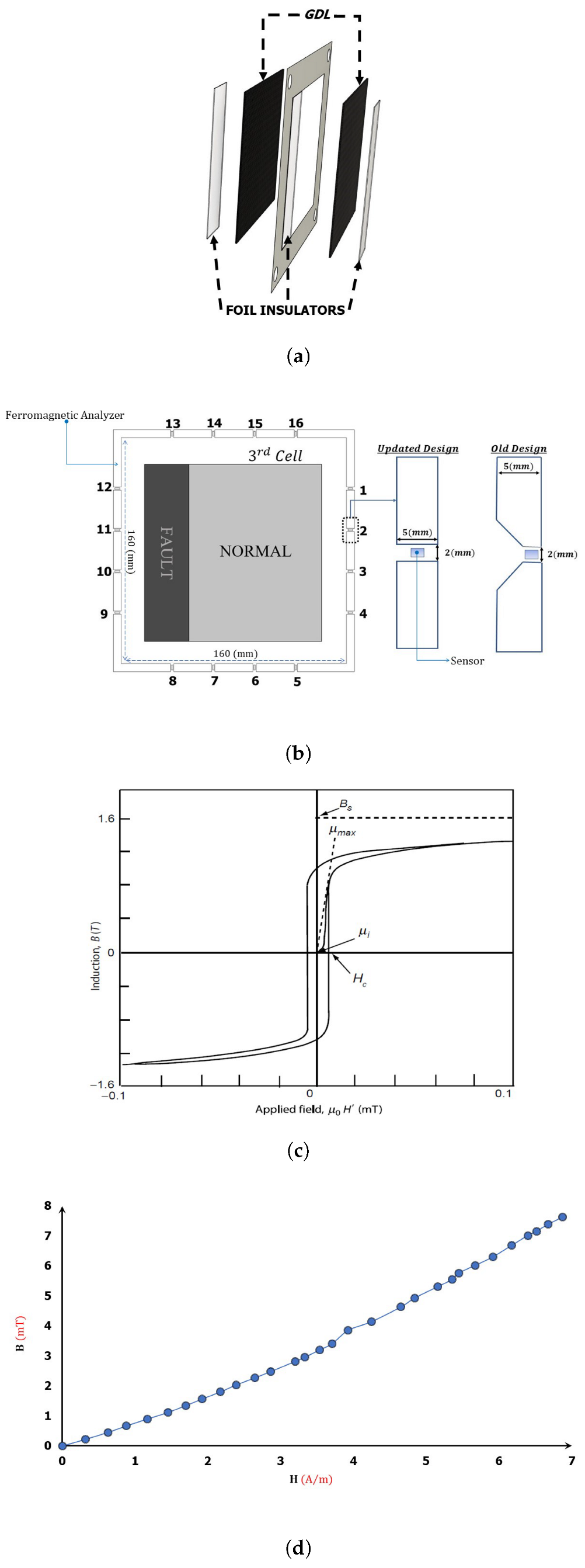
3.1. Experimental Setup and Results

To obtain a current distribution comparable to that inside the FC volume, Figure 7 presents the test bench created to hold the ferromagnetic analyzer around the simplified emulator, which has similar geometry and structure as an actual FC stack. This emulator consists of a passivized PEMFC stack of five cells connected with two copper bars at both end plates levels, see Figure 7. These bars are used to supply the emulator by $I_{stack}=70$ A. To allow electron current flow, for each cell, in the MEA, only two conductive GDLs were used instead of the MEA presented in Section 2.1. The electrolyte membrane involving five layers, see Figure 1a, has been disposed and the two GDL are kept in the passivized FC.

In this experiment, the conduction fault covering $25\%$ of the third cell active area is realized by three polyethylene insulator foil positioned to the left of the GDL of the third cell of the stack. These insulators have been inserted at the front, middle, and back of the two GDLs to ensure that the current will not flow through this faulty area, see Figure 8a.

The stack was tested for both normal and faulty behavior in the presence of 160 (mm) × 160 (mm) ferromagnetic magnetic analyzer with 3 (mm) thickness. The design of the magnetic analyzer presented in Figure 7 and Figure 8b has been improved by increasing the sensor air gap area from 6 mm² used in [53] up to 15 mm² in the updated design.

One important aspect to model the magnetic field analyzer was to take into consideration the specific magnetic behavior of a soft ferromagnetic material, especially for a low magnitude of the internal magnetic field intensity. As shown in Figure 8c [59], the initial permeability, ${\mu }_i$, at the origin of the hysteresis loop is smaller than the maximum permeability value, ${\mu }_{max}$, attained for a slightly larger intensity of the magnetic field. Therefore, the real characteristic of the mumetal material composing the ferromagnetic circuit of the analyzer has been experimentally characterized, by measuring the magnetic flux density in the airgap of a toroidal core, with helical winding. The obtained characteristic $B\left(H\right)$ shown in Figure 8d has been realized for a very low magnitude of the flux density, lower than $10mT$, which is in the range of the magnetic analyzer measurements. In this interval, the $B\left(H\right)$ can be considered linear B = ${\mu }_0{\mu }_{r}H$ with an average value of the relative permeability ${\mu }_{rFerro}$ = 741, much lower than the maximum value of the mumetal relative permeability catalog value ${\mu }_{max}$ = ${10}^5$.

We observed by FEM analysis that this modification allows measuring the same magnetic field at the sensor level with the advantage of a larger volume in the airgap and with a homogeneous magnetic field. In this way, the insertion of the sensors in the airgap will be easier because the imperfections in the position of the sensors will have less influence on the measured magnetic field. The magnetic analyzer was placed at three different positions, around $cell$ 2, $cell$ 3, and $cell$ 4, see Figure 6 to measure the external magnetic field generated. This analyzer is based on a high permeability material, Mu-metal ferromagnetic, which is a soft material nickel-iron alloy with 16 non-magnetic air gaps in which the linear Hall effect (SS94A1F-type) sensors were inserted. This type of sensor was characterized by an output voltage of 4 V at zero magnetic flux density with a high sensitivity of 25 mV/G. The 16 output voltages proportional to the magnetic field magnitude measured by the sensors are collected by a National Instrument NI 9205 data acquisition system and Lab-VIEW software. This data acquisition provides 32 analog inputs with an input ADC (Analog to Digital Converter) resolution of 16 bits. The experimental measurements recorded the magnetic field magnitude measured by the magnetic sensors $B=[B_1,B_2,\dots ,B_{16}]$ placed in the ferromagnetic analyzer air gap.

The stack was powered by a power source controlled at EP levels to ensure an overall stack current of 70 A. Magnetic field measurements were performed in both operating modes for the emulator, the normal behavior as $B_{Normal}=[B_{N1},B_{N2},\dots ,B_{N16}]$ and conduction fault behavior as $B_{Fault}=[B_{F1},B_{F2},\dots ,B_{F16}]$ at the different analyzer positions. Figure 9a represents the magnetic field magnitude of the passivized stack behavior under normal and faulty conditions when the ferromagnetic analyzer is around the affected cell (Position 3). To test the change in the internal j between normal and faulty operation, $\Delta B=B_{Normal}-B_{Fault}$ must be analyzed.

Figure 9b,c allow us to compare $\Delta B$ measured on the 3D emulator and the $\Delta B$ obtained on the 2D emulator presented in [53] for the same fault type and position (left of the active area). A lower amplitude of a spatial $\Delta B$ signal measured on the 3D emulator Figure 9b compared to the 2D emulator Figure 9c can be explained by a local deviation of the current distribution along the main axis for a 3D conduction fault, while in the case of the 2D emulator, the conduction fault concerns a larger volume because the fault is uniform along the main axis. The positive $\Delta B$ is explained by the drop of the magnetic field for the sensors located close to the conduction fault in which the current is 0 A, and the negative $\Delta B$ values are obtained for the sensors close to the normal part of the active zone, see Figure 8b. This phenomenon is due to the conservative global current density, which leads to a current drop at the faulty part and increases in the rest of the conductive part of the FC.

3.2. Numerical Modeling and Results

Based on the experimental findings, the numerical model is developed to justify the 3D fault detection use. During the faulty conditions, the external field is measured with different analyzer positions, around Cell 2, Cell 3, and Cell 4. Subsequently, the experimental result of $\Delta B$ is fairly compared with the simulation when the circuit analyzer is around cell 3 to highlight the accuracy of the proposed emulator. This numerical model is based on the strong coupling between the electrical conduction application that solves the current density flow inside the FC emulator and the magnetic application that calculates the internal and external magnetic field generated from the internal current density flow in the emulator domain.

3.2.1. Coupled Electric Conduction and Magnetic Formulations

The numerical model of the FC emulator conductive domain coupled in a circuit with a current source, as previously presented in Figure 5a has as its objective to compute both current distribution J inside the conductive domain, as well as to compute the magnetic flux density distribution B inside and around the conductive domain.

The equations describing both electrical conduction and magnetic formulations are included in the Faraday Law Equation (8), the Gauss law for the magnetic flux Equation (9), and the ampere theorem Equation (10). Two other equations are related to electrical and magnetic behavior: the theorem of the electrical conduction Equation (11) and $B\left(H\right)$ dependency Equation (12)

$$curl(\overrightarrow{E})=-(\frac{\partial \overrightarrow{B}}{\partial t})$$

(8)

$$div(\overrightarrow{B})=0$$

(9)

$$curl(\overrightarrow{H})=\overrightarrow{j}$$

(10)

$$\overrightarrow{j}=\sigma \overrightarrow{E}$$

(11)

$$\overrightarrow{B}=\mu \overrightarrow{H}$$

(12)

where E is the electric field in (V/m), B the magnetic field in (T), H the magnetic field strength in (A/m), $\mu$ the permeability in (H/m), V the electric potential in (V), j the current density in (A/m²) and $\sigma$ the conductivity in (S).

A cylindrical domain has been considered around the FC emulator and external to the magnetic circuit analyzer; see Figure 10. To solve the problem using the FE (Finite Element) method, on the domain borders, two boundary conditions were specified: tangent magnetic field and normal electric field.

A 3D FEM formulation based on magnetic scalar potential, which is included in Altair Flux software, has been chosen to solve the coupled electric conduction and magnetic equations. As shown in [60], magnetic scalar has good performance for solving problems containing nonlinear massive conductors coupled with circuit equations.

Therefore, this method is adapted as we consider 3D conduction defaults as included in the conductive domain of the FC emulator. At the electrolyte membrane level, it was also possible to simulate the realistic behavior of the FC emulator by using the electric field characteristics $E\left(j\right)$, see Figure 5b, and as the magnetic scalar potential formulation also allows one to take in consideration the conduction nonlinearities.

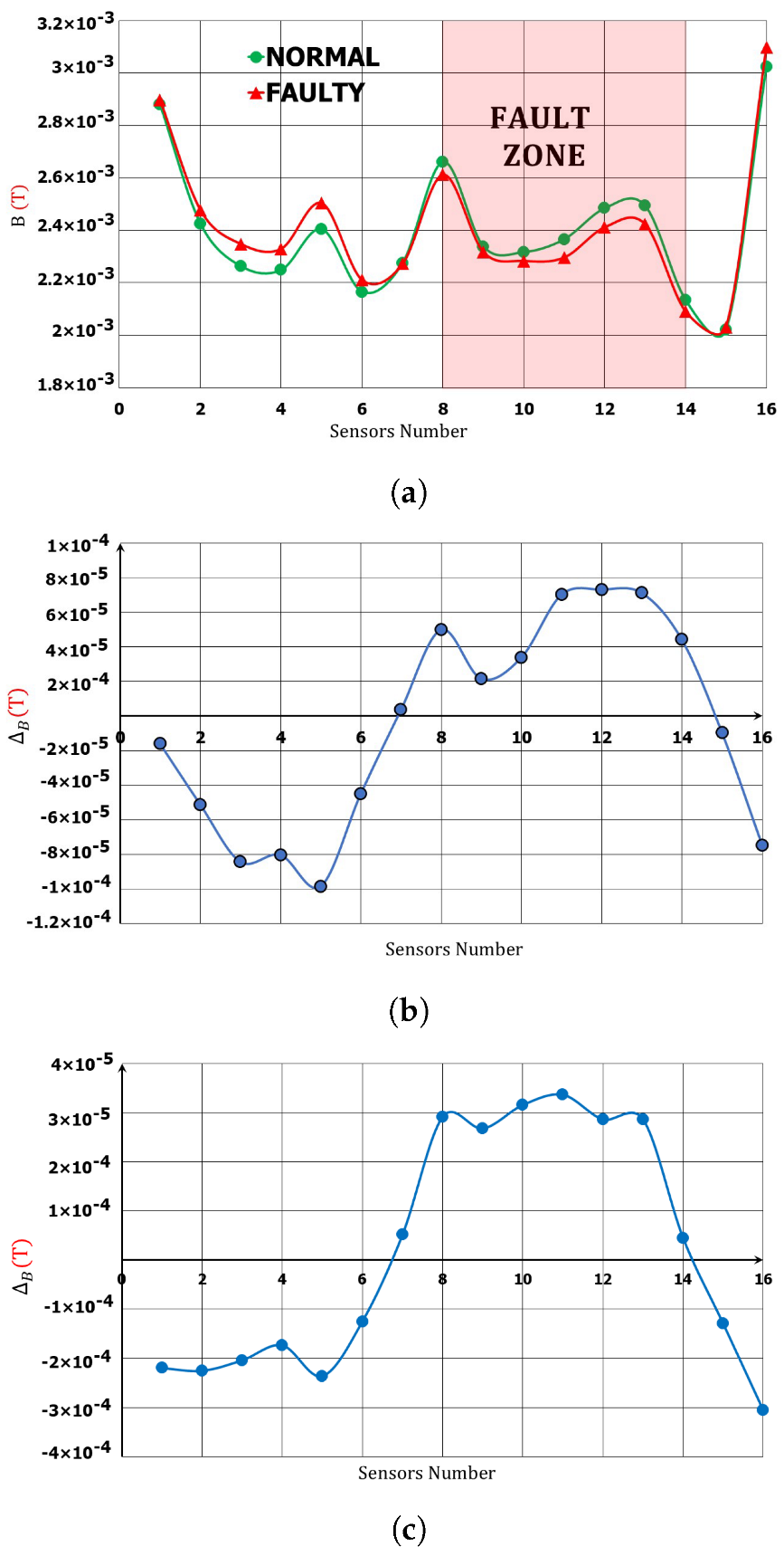
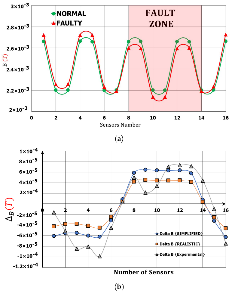
3.2.2. Fault Cell Detection Using Magnetic Field Measurements

In this section, a fault of the simplified model like the one explained in the experimental section has been used by considering an affected $25\%$ of the left active area of the third cell in the stack, and a ferromagnetic analyzer around the stack with 16 air-gap to attach the magnetic sensors, to measure the external magnetic field around each cell Figure 7 across different analyzer positions Figure 6. The fault was considered as an insulator to block the current flow through the affected part of the active area. Figure 11 illustrates the heterogeneous current density distribution in the faulty state operation of the PEMFC stack. We can observe the current density magnitude in the transversal cut plane (ZOX) at the level of the 3rd cell; see Figure 11a. This fault may affect neighboring cells (cell 2 and cell 4) due to the short distance between these cells and the position of the fault, thereby resulting in a more heterogeneous current density within these cells as compared to the other cells, see Figure 11b. Figure 11c illustrates the current density distribution flow viewed on the longitudinal (YOX) cut plane.

In this study, the multivariate observations between different analyzer positions are given by a vector of $\Delta B_s$ that is measured by the magnetic sensors in both emulator behaviors and the Euclidean distance exposed in Equation (13), where $n_s=16$, the number of the magnetic sensors inside the analyzer.

$$\mathcal{E}=\sqrt{\sum _{i=1}^{n_s}(\Delta B_{s_i}{)}^2}$$

(13)

Figure 12a illustrates the magnetic fields obtained in simulation, which explains the simplified model in the two behaviors of the emulator, normal and faulty. The perfect symmetry of the distribution of the sensors around the stack leads to a wavy magnetic field distribution around a single cell. Moreover, measuring the magnetic field using the circuit analyzer will inversely affect the magnetic sensors so that the sensors located near the center side of the analyzer (S2, S3) read a lower magnetic value compared to (S1, S4) Figure 8a located near the edges of the analyzer. This phenomenon is due to the presence of the ferromagnetic material and a bigger magneto-motive force received at the level of the corner components of the magnetic circuit analyzer. Furthermore, the ${\Delta }_B$ result of comparing the simulation (simplified and realistic) and experimental at Position 3 Figure 6 of the circuit analyzer are presented in Figure 12b. We can observe that ${\Delta }_B$ has a similar shape between simulations and the experimental emulator. The positive $\Delta B$ represents the magnetic field drop for the sensors located near the fault line zone, where the current in the affected part drops, resulting in an increase in the current density flux producing a negative $\Delta B$ in the remaining unaffected part.

On another hand, the experimental and simulated 3D magnetic field faulty detection for ${\mathcal{E}}_{experimental}$ and ${\mathcal{E}}_{simulated}$ are presented in Figure 13a and Figure 13b, respectively. The maximum value of the average $\mathcal{E}$ is around the fault position (cell 3) in both simulated and experimental models and starts to decrease near the affected neighbor cells, which become far from the position of the fault. This is due to the current drop in the fault region at the third cell, which also affects the flow of the current inside the near cells.

4. Conclusions

The objective of this work was to develop the FC noninvasive diagnostic methodology based on the measurement of the external magnetic field surrounding the stack. After a literature review on FC diagnostic and on FC current distribution assessment, an improved magnetic analyzer has been proposed. This analyzer amplifies the magnetic field around the cell to perform an accurate detection of the fault position.

The main contribution of this work was the concept of an innovative fuel cell magnetic field emulator specially designed to duplicate current density distribution and the produced magnetic field of a real FC stack. Based on a passivized FC structure, supplied by a current source, this emulator reproduces an equivalent current distribution in a similar geometrical domain, as the current distribution inside a Fuel Cell domain, during its steady-state operation. As the current distribution represents the source of the magnetic field produced by the FC, the emulator will also replicate the magnetic field of a real FC. Multi-physical modeling of an FC involving couplings between electrochemical, electric, and magneto-static models has been realized in normal and faulty operation and integrated into the physical description of the emulator regions.

Another key point was to validate the magnetic field analyzer and the methodology for realistic 3D local faults inside the FC stack emulator. The emulator has been involved in the realization of numerical simulations and experimental analysis to prove the ability of the system to detect 3D faults. Once, the experimental measurements of the flux density, provided by the magnetic analyzer positioned around the fault position, are coherent with the numerical simulation results. Moreover, the multivariate distance between the magnetic measurements expressed in (13), realized around the cells in fault and normal operation, shows an encouraging result to detect the fault position inside the FC stack. Therefore, the diagnostic procedure will include a set of magnetic field measurements for different positions of the magnetic analyzer along the FC stack main axis, to taste the state of health of each cell.

Adapted to finite element analysis, owing to its low experimental cost, the proposed emulator is expected to be a good candidate for developing further diagnostic algorithms based on the measurement of the external magnetic field surrounding the FC stack. Being able to reproduce the magnetic signatures for different localization and for different fault shapes inside the FC stack, both the numerical model and the emulator will be useful calibration of model-based and data-based diagnostic algorithms. A further comparative study will analyze the emulator and multi-physical model for different operating faults (membrane degradation, flooding, drying, under stoichiometry) of an actual FC.

References

1. Perry, M.; Fuller, T. A historical perspective of fuel cell technology in the 20th century. J. Electrochem. Soc. 2002, 149, S59. [Google Scholar] [CrossRef]
2. Mock, P.; Schmid, S. Fuel cells for automotive powertrains—A techno-economic assessment. J. Power Sources 2009, 190, 133–140. [Google Scholar] [CrossRef] [Green Version]
3. Minelli, S.; Civelli, M.; Rondinini, S.; Minguzzi, A.; Vertova, A. Aemfc exploiting a pd/ceo2-based anode compared to classic pemfc via lca analysis. Hydrogen 2021, 2, 246–261. [Google Scholar] [CrossRef]
4. Handwerker, M.; Wellnitz, J.; Marzbani, H. Comparison of hydrogen powertrains with the battery powered electric vehicle and investigation of small-scale local hydrogen production using renewable energy. Hydrogen 2021, 2, 76–100. [Google Scholar] [CrossRef]
5. Lambert, H.; Roche, R.; Jeme, S.; Ortega, P.; Hissel, D. Combined cooling and power management strategy for a standalone house using hydrogen and solar energy. Hydrogen 2021, 2, 207–224. [Google Scholar] [CrossRef]
6. Gurz, M.; Baltacioglu, E.; Hames, Y.; Kaya, K. The meeting of hydrogen and automotive: A review. Int. J. Hydrog. Energy 2017, 42, 23334–23346. [Google Scholar] [CrossRef]
7. Wilberforce, T.; Alaswad, A.; Palumbo, A.; Dassisti, M.; Olabi, A.-G. Advances in stationary and portable fuel cell applications. Int. J. Hydrog. Energy 2016, 41, 16509–16522. [Google Scholar] [CrossRef] [Green Version]
8. Andrews, J.; Shabani, B. Re-envisioning the role of hydrogen in a sustainable energy economy. Int. J. Hydrog. Energy 2012, 37, 1184–1203. [Google Scholar] [CrossRef]
9. Knights, S.; Colbow, K.; St-Pierre, J.; Wilkinson, D. Aging mechanisms and lifetime of pefc and dmfc. J. Power Sources 2004, 127, 127–134. [Google Scholar] [CrossRef]
10. Taniguchi, A.; Akita, T.; Yasuda, K.; Miyazaki, Y. Analysis of electrocatalyst degradation in pemfc caused by cell reversal during fuel starvation. J. Power Sources 2004, 130, 42–49. [Google Scholar] [CrossRef]
11. Liu, Z.; Yang, L.; Mao, Z.; Zhuge, W.; Zhang, Y.; Wang, L. Behavior of pemfc in starvation. J. Power Sources 2006, 157, 166–176. [Google Scholar] [CrossRef]
12. Tang, H.; Peikang, S.; Wang, F.; Pan, M. A degradation study of nafion proton exchange membrane of pem fuel cells. J. Power Sources 2007, 170, 85–92. [Google Scholar] [CrossRef]
13. Husar, A.; Serra, M.; Kunusch, C. Description of gasket failure in a 7 cell pemfc stack. J. Power Sources 2007, 169, 85–91. [Google Scholar] [CrossRef] [Green Version]
14. Yue, M.; Jemei, S.; Gouriveau, R.; Zerhouni, N. Review on health-conscious energy management strategies for fuel cell hybrid electric vehicles: Degradation models and strategies. Int. J. Hydrog. Energy 2019, 44, 6844–6861. [Google Scholar] [CrossRef]
15. Wang, J.; Yang, B.; Zeng, C.; Chen, Y.; Guo, Z.; Li, D.; Shao, R.; Shu, H.; Yu, T. Recent advances and summarization of fault diagnosis techniques for proton exchange membrane fuel cell systems: A critical overview. J. Power Sources 2021, 500, 229932. [Google Scholar] [CrossRef]
16. Tian, G.; Wasterlain, S.; Endichi, I.; Candusso, D.; Harel, F.; François, X.; Péra, M.-C.; Hissel, D.; Kauffmann, J.-M. Diagnosis methods dedicated to the localisation of failed cells within pemfc stacks. J. Power Sources 2008, 182, 449–461. [Google Scholar] [CrossRef]
17. Veziroglu, A.; Macario, R. Fuel cell vehicles: State of the art with economic and environmental concerns. Int. J. Hydrog. Energy 2011, 36, 25–43. [Google Scholar] [CrossRef]
18. Rubio, M.A.; Urquia, A.; Dormido, S. Diagnosis of performance degradation phenomena in pem fuel cells. Int. J. Hydrog. Energy 2010, 35, 2586–2590. [Google Scholar] [CrossRef]
19. Chevalier, S.; Trichet, D.; Auvity, B.; Olivier, J.C.; Josset, C.; Machmoum, M. Multiphysics dc and ac models of a pemfc for the detection of degraded cell parameters. Int. J. Hydrog. Energy 2013, 38, 11609–11618. [Google Scholar] [CrossRef]
20. Petrone, R.; Zheng, Z.; Hissel, D.; Péra, M.-C.; Pianese, C.; Sorrentino, M.; Béchérif, M.; Yousfi-Steiner, N. A review on model-based diagnosis methodologies for pemfcs. Int. J. Hydrog. Energy 2013, 38, 7077–7091. [Google Scholar] [CrossRef]
21. Escobet, T.; Feroldi, D.; De Lira, S.; Puig, V.; Quevedo, J.; Riera, J.; Serra, M. Model-based fault diagnosis in pem fuel cell systems. J. Power Sources 2009, 192, 216–223. [Google Scholar] [CrossRef] [Green Version]
22. Hissel, D.; Péra, M.C.; Kauffmann, J.M. Diagnosis of automotive fuel cell power generators. J. Power Sources 2004, 128, 239–246. [Google Scholar] [CrossRef]
23. Hua, J.; Li, J.; Ouyang, M.; Lu, L.; Xu, L. Proton exchange membrane fuel cell system diagnosis based on the multivariate statistical method. Int. J. Hydrog. Energy 2011, 36, 9896–9905. [Google Scholar] [CrossRef]
24. Yousfi Steiner, N.; Hissel, D.; Moçotéguy, P.; Candusso, D. Diagnosis of polymer electrolyte fuel cells failure modes (flooding & drying out) by neural networks modeling. Int. J. Hydrog. Energy 2011, 36, 3067–3075. [Google Scholar]
25. Zheng, Z.; Petrone, R.; Péra, M.-C.; Hissel, D.; Béchérif, M.; Pianese, C.; Yousfi Steiner, N.; Sorrentino, M. A review on non-model based diagnosis methodologies for pem fuel cell stacks and systems. Int. J. Hydrog. Energy 2013, 38, 8914–8926. [Google Scholar] [CrossRef]
26. Giurgea, S.; Tirnovan, R.; Hissel, D.; Outbib, R. An analysis of fluidic voltage statistical correlation for a diagnosis of pem fuel cell flooding. Int. J. Hydrog. Energy 2013, 38, 4689–4696. [Google Scholar] [CrossRef]
27. Chen, H.; Zhao, X.; Qu, B.; Zhang, T.; Pei, P.; Li, C. An evaluation method of gas distribution quality in dynamic process of proton exchange membrane fuel cell. Appl. Energy 2018, 232, 26–35. [Google Scholar] [CrossRef]
28. Yuan, X.-Z.R.; Song, C.; Wang, H.; Zhang, J. Electrochemical Impedance Spectroscopy in PEM Fuel Cells: Fundamentals and Applications; Springer Science & Business Media: New York, NY, USA, 2009. [Google Scholar]
29. Brunetto, C.; Moschetto, A.; Tina, G. Pem fuel cell testing by electrochemical impedance spectroscopy. Electr. Power Syst. Res. 2009, 79, 17–26. [Google Scholar] [CrossRef]
30. Huang, Q.-A.; Hui, R.; Wang, B.; Zhang, J. A review of ac impedance modeling and validation in sofc diagnosis. Electrochim. Acta 2007, 52, 8144–8164. [Google Scholar] [CrossRef]
31. Niya, S.M.R.; Hoorfar, M. Study of proton exchange membrane fuel cells using electrochemical impedance spectroscopy technique—A review. J. Power Sources 2013, 240, 281–293. [Google Scholar] [CrossRef]
32. Sui, P.-C.; Zhu, X.; Djilali, N. Modeling of pem fuel cell catalyst layers: Status and outlook. Electrochem. Energy Rev. 2019, 2, 428–466. [Google Scholar] [CrossRef]
33. Wang, R.; Wang, H.; Luo, F.; Liao, S. Core–shell-structured low-platinum electrocatalysts for fuel cell applications. Electrochem. Energy Rev. 2018, 1, 324–387. [Google Scholar] [CrossRef]
34. Depernet, D.; Narjiss, A.; Gustin, F.; Hissel, D.; Péra, M.-C. Integration of electrochemical impedance spectroscopy functionality in proton exchange membrane fuel cell power converter. Int. J. Hydrog. Energy 2016, 41, 5378–5388. [Google Scholar] [CrossRef]
35. Robin, C.; Gerard, M.; d’Arbigny, J.; Schott, P.; Jabbour, L.; Bultel, Y. Development and experimental validation of a pem fuel cell 2d-model to study heterogeneities effects along large-area cell surface. Int. J. Hydrog. Energy 2015, 40, 10211–10230. [Google Scholar] [CrossRef]
36. Geske, M.; Heuer, M.; Heideck, G.; Styczynski, Z. Current density distribution mapping in pem fuel cells as an instrument for operational measurements. Energies 2010, 3, 770–783. [Google Scholar] [CrossRef] [Green Version]
37. Candusso, D.; Poirot-Crouvezier, J.P.; Bador, B.; Rullière, E.; Soulier, R.; Voyant, J.Y. Determination of current density distribution in proton exchange membrane fuel cells. Eur. Phys. J.-Appl. Phys. 2004, 25, 67–74. [Google Scholar] [CrossRef]
38. Peng, L.; Shao, H.; Qiu, D.; Yi, P.; Lai, X. Investigation of the non-uniform distribution of current density in commercial-size proton exchange membrane fuel cells. J. Power Sources 2020, 453, 227836. [Google Scholar] [CrossRef]
39. Nishikawa, H.; Kurihara, R.; Sukemori, S.; Sugawara, T.; Kobayasi, H.; Abe, S.; Aoki, T.; Ogami, Y.; Matsunaga, A. Measurements of humidity and current distribution in a pefc. J. Power Sources 2006, 155, 213–218. [Google Scholar] [CrossRef]
40. Nasu, T.; Matsushita, Y.; Okano, J.; Okajima, K. Study of current distribution in pemfc stack using magnetic sensor probe. J. Int. Counc. Electr. Eng. 2012, 2, 391–396. [Google Scholar] [CrossRef]
41. Akimoto, Y.; Okajima, K.; Uchiyama, Y. Evaluation of current distribution in a pemfc using a magnetic sensor probe. Energy Procedia 2015, 75, 2015–2020. [Google Scholar] [CrossRef] [Green Version]
42. Gerard, M.; Poirot-Crouvezier, J.-P.; Hissel, D.; Pera, M.-C. Oxygen starvation analysis during air feeding faults in pemfc. Int. J. Hydrog. Energy 2010, 35, 12295–12307. [Google Scholar] [CrossRef]
43. Simulation Services. Available online: http://splusplus.com (accessed on 3 March 2022).
44. Hauer, K.-H.; Potthast, R.; Wüster, T.; Stolten, D. Magnetotomography—A new method for analysing fuel cell performance and quality. J. Power Sources 2005, 143, 67–74. [Google Scholar] [CrossRef]
45. Hamaz, T.; Cadet, C.; Druart, F.; Cauffet, G. Diagnosis of pem fuel cell stack based on magnetic fields measurements. IFAC Proc. Vol. 2014, 47, 11482–11487. [Google Scholar] [CrossRef] [Green Version]
46. Le Ny, M.; Chadebec, O.; Cauffet, G.; Dedulle, J.-M.; Bultel, Y.; Rosini, S.; Fourneron, Y.; Kuo-Peng, P. Current distribution identification in fuel cell stacks from external magnetic field measurements. IEEE Trans. Magn. 2013, 49, 1925–1928. [Google Scholar] [CrossRef] [Green Version]
47. Le Ny, M.; Chadebec, O.; Cauffet, G.; Rosini, S.; Bultel, Y. Pemfc stack diagnosis based on external magnetic field measurements. J. Appl. Electrochem. 2015, 45, 667–677. [Google Scholar] [CrossRef]
48. Ifrek, L.; Chadebec, O.; Rosini, S.; Cauffet, G.; Bultel, Y.; Bannwarth, B. Fault identification on a fuel cell by 3-d current density reconstruction from external magnetic field measurements. IEEE Trans. Magn. 2019, 55, 1–5. [Google Scholar] [CrossRef]
49. Ifrek, L.; Rosini, S.; Cauffet, G.; Chadebec, O.; Rouveyre, L.; Bultel, Y. Fault detection for polymer electrolyte membrane fuel cell stack by external magnetic field. Electrochim. Acta 2019, 313, 141–150. [Google Scholar] [CrossRef]
50. Li, Z.; Cadet, C.; Outbib, R. Diagnosis for pemfc based on magnetic measurements and data-driven approach. IEEE Trans. Energy Convers. 2018, 34, 964–972. [Google Scholar] [CrossRef]
51. Liu, Z.; Sun, Y.; Mao, L.; Zhang, H.; Jackson, L.; Wu, Q.; Lu, S. Efficient fault diagnosis of proton exchange membrane fuel cell using external magnetic field measurement. Energy Convers. Manag. 2022, 266, 115809. [Google Scholar] [CrossRef]
52. LaManna, J.M.; Chakraborty, S.; Gagliardo, J.J.; Mench, M.M. Isolation of transport mechanisms in pefcs using high resolution neutron imaging. Int. J. Hydrog. Energy 2014, 39, 3387–3396. [Google Scholar] [CrossRef]
53. Plait, A.; Giurgea, S.; Hissel, D.; Espanet, C. New magnetic field analyzer device dedicated for polymer electrolyte fuel cells noninvasive diagnostic. Int. J. Hydrog. Energy 2020, 45, 14071–14082. [Google Scholar] [CrossRef]
54. Le Ny, M.; Chadebec, O.; Cauffet, G.; Dedulle, J.-M.; Bultel, Y. A three dimensional electrical model of pemfc stack. Fuel Cells 2012, 12, 225–238. [Google Scholar] [CrossRef]
55. Larminie, J.; Dicks, A.; McDonald, M.S. Fuel Cell Systems Explained; J. Wiley: Chichester, UK, 2003; Volume 2. [Google Scholar]
56. Görgün, H.; Arcak, M.; Barbir, F. An algorithm for estimation of membrane water content in pem fuel cells. J. Power Sources 2006, 157, 389–394. [Google Scholar] [CrossRef]
57. Altair®, User Guide Flux® 12.3. 2020, Volume 3. Available online: http://www.altair.com/flux (accessed on 3 March 2022).
58. Ifrek, L.; Cauffet, G.; Chadebec, O.; Bultel, Y.; Rosini, S.; Rouveyre, L. 2d and 3d fault basis for fuel cell diagnosis by external magnetic field measurements. Eur. Phys. J. Appl. Phys. 2017, 79, 20901. [Google Scholar] [CrossRef] [Green Version]
59. Coey, J.M.D. Magnetism and Magnetic Materials; Cambridge University Press: Cambridge, UK, 2010. [Google Scholar]
60. Meunier, G.; Le Floch, Y.; Guérin, C. A nonlinear circuit coupled tt/sub 0/-/spl phi/formulation for solid conductors. IEEE Trans. Magn. 2003, 39, 1729–1732. [Google Scholar] [CrossRef]
Figure 1. (a) FC structure (1) Bipolar Plates (BP), (2) Polymer Electrolyte Membrane (PEM), (3) Thin conductive catalyst, (4) Gas Diffusion Layer (GDL) with (b) the electro-chemical representation.
Hydrogen 04 00003 g001
Figure 2. FC polarization curve. The dotted red lines indicate the limits of V i n v m i n , E r e v , and j m a x .
Hydrogen 04 00003 g002
Figure 3. Discretized current density corresponding to n surface elements at the electrolyte level (a), electric circuit representation for the current density distribution inside FC (b).
Hydrogen 04 00003 g003
Figure 4. Passivized FC.
Hydrogen 04 00003 g004
Figure 5. (a) Equivalent electric circuit of the passivized FC, (b) membrane electric field characteristics of the realistic and simplified emulator.
Hydrogen 04 00003 g005
Figure 6. Different analyzer positions across z-axis.
Hydrogen 04 00003 g006
Figure 7. Passivized FC (a) test bench, (b) stack and magnetic analyzer circuit.
Hydrogen 04 00003 g007
Figure 8. (a) Active area with the fault type, (b) circuit analyzer with sensors, (c) difference between μ i and μ m a x for soft magnetic materials [59], and (d) characterization of the ferromagnetic material used in the analyzer.
Hydrogen 04 00003 g008
Figure 9. Experimental representation for (a) normal and fault passivated FC emulator, with (b) the fabricated 3D Δ B and (c) 2D Δ B produced by 16 bars emulator.
Hydrogen 04 00003 g009
Figure 10. FEM passivized FC.
Hydrogen 04 00003 g010
Figure 11. Current density distribution in faulty condition (a) cut plane (ZOX) at the level of 3rd cell, (b) cut plane (ZOX) at the level of 2nd and 4th cells, (c) cut plane (XOY).
Hydrogen 04 00003 g011
Figure 12. (a) Simulated simplified model in normal and faulty behaviors of the 3rd cell, (b) Δ B simulation (simplified and realistic) and experimental at the level of the 3rd cell.
Hydrogen 04 00003 g012
Figure 13. (a) Experimental 3D fault detection, (b) simulation 3D fault detection.
Hydrogen 04 00003 g013