A Parametric Study on the LDB Strength of Steel-Concrete Composite Beams

Abstract

Lateral distortional buckling (LDB) is an instability phenomenon characteristic of steel-concrete composite beams (SCCB) that occurs in the presence of hogging moments in regions close to internal supports. The LDB behavior in SCCB is not yet fully understood. The procedures for determining the LDB strength are based on the classic lateral torsional buckling theory or on the inverted U-frame model. In addition, the standard procedures make use of the classic design curves of the SSRC (Structural Stability Research Council) and ECCS (European Convention for Constructional Steelwork) developed to analyze the stability behavior of steel elements. However, studies indicate that the use of the same empirical curves obtained for the analysis of steel elements leads to the conservative results of the LDB strength in SCCB. Therefore, this article aims to assess the LDB strength in SCCB through the development of post-buckling numerical analysis using the ABAQUS software. In the parametric study, four types of steel with different mechanical properties were analyzed. In addition, the I-section, the unrestrained length, and the reinforcement rate in the concrete slab were varied. The results showed the influence of the steel type on the LDB strength and deviations from the standard procedures. A small influence of the longitudinal reinforcement area variation was verified in the LDB strength in the FE analyses; however, this factor is significantly important in the standard procedures, causing considerable divergences. These results can provide a reference for future research and specification reviews.

1. Introduction

Lateral distortional buckling (LDB) is an instability failure mode of steel-concrete composite beams (SCCB) under hogging moments [1,2,3,4,5,6]. As shown in Figure 1, LDB is characterized by a lateral displacement (δ) accompanied by a rotation (θ) of the compressed bottom flange that occurs due to the web distortion, if it is not rigid enough to withstand the lateral bending [7,8,9].

This instability phenomenon is responsible for reducing the strength of continuous and semi-continuous SCCB [10,11]. However, in addition to the occurrence of LDB, SCCB under the action of hogging moment may be subject to local stability modes, such as the flange local buckling (FLB), and even a combination of LDB and local modes [1]. The LDB phenomenon in SCCB is generally conservatively assessed in the standard codes as being a type of LTB. However, Bradford and Johnson [12] showed that LDB strength in SCCB can be more than doubled in many cases when compared to LTB strength. The LDB in SCCB can also be analyzed through the inverted U-frame method. In this method, the bottom compression flange of the I-section is considered as a strut compressed uniformly along its length by the maximum bending stress that is induced in it, and which is restrained by a continuous Winkler spring whose stiffness is that of the web in the plane of its cross-section acting as a cantilever (Figure 2) [1,2,3].

In general, to determine the LDB strength of SCCB, current standard procedures require the determination of the elastic distortional critical moment. In the previous version of EC4 [13] (EN 1994-1-1:1992), the methodology proposed by Roik et al. [14] to determine the elastic distortional critical moment was adopted. This methodology is still used in the Brazilian code [15] (ABNT NBR 8800:2008). After determining the elastic distortional critical moment the standard code such as Eurocode 4 [13], NBR 8800:2008 [15], AISC [16], and Australian codes [17] make use of the same design curves proposed for steel elements to determine the LDB strength of SCCB. However, studies [18,19,20] have shown divergences between the results of elastic distortional critical moments, obtained through numerical analysis, when compared with the methodologies proposed by Roik et al. [14], Svensson [21], William and Jemah [22], and Hanswille et al. [23]. Therefore, the use of these methodologies for the estimation of the elastic distortional critical moment can result in the mistaken obtaining of the strength of SCCB under hogging moments by standard procedures. In addition, Zhou and Yan [4], Liu et al. [9], and Rossi et al. [3] showed very conservative situations in the standard codes when compared with FEA results obtained for SCCB subjected to uniform hogging moment.

In a recent publication, Rossi et al. [3] present a critical review of LDB in SCCB. The authors showed that the LDB investigations emphasized analyzing the LDB elastic behavior [1,2,24,25,26,27,28,29,30,31,32,33,34,35], in an attempt to obtain a method for determining the elastic critical moment, or sought to analyze the LDB strength of SCCB [1,4,8,9,10,11,26,27,29,30,31,36,37,38]. The authors showed that there are considerable divergences between the existing methodologies for determining the elastic critical moment. In addition, Rossi et al. [3] presented disagreements between experimental results and post-buckling numerical analysis when compared with standard procedures. Finally, the researchers present the need for further investigations on SCCB under the action of the hogging moment. Previous investigations by Rossi et al. [1,32,33] showed that LDB in steel-concrete composite beams is not fully resolved and there is a need for further investigations on the subject. One of the parameters to be investigated is the influence of the steel mechanical characteristics of the I-beams on the LDB behavior. The need to analyze the influence of the yield strength of different types of steel on the LDB phenomenon can be seen in Zhao, Li and Sun [34], and Sun et al. [35]. In these works, the authors verified that important standard procedures underestimate the resistance to global instability of singly symmetric I-sections with high-strength steels (HSS).

In this way, although there is a considerable number of investigations about the LDB phenomenon in SCCB, no study has investigated the possible influence of different types of steel and their mechanical properties (f_y and f_u) on the LDB strength of SCCB. Even though standard procedures consider indirectly, through the slenderness ratio ($\lambda =\sqrt{\frac{M_{cr}}{M_{pl}}}$), the yield strength of the steel sections, no comparative study was carried out between the LDB strength obtained for different types of steel in numerical analyses with the SSRC and ECCS design curves used to verify the LDB strength of SCCB. In addition, no study on the LDB strength of SCCB has thoroughly investigated the influence of the longitudinal reinforcement area variation in the concrete slab and the behavior of standard procedures in relation to this parameter. Therefore, this article aims to assess the LDB strength of SCCB through the development of post-buckling numerical analysis with the Dassault Systèmes ABAQUS 6.14 [38] software. In the post-buckling numerical analysis, the initial geometric imperfection, residual stress, real shear connector, geometric nonlinearity, and material nonlinearity were considered through the numerical model developed. The SCCB analyzed are simply supported, with restrictions on lateral slab displacement, and are subjected to a uniform hogging moment distribution. In the parametric study, four types of steel with different mechanical properties were analyzed. In addition, the I-section, the unrestrained length, and the reinforcement rate in the concrete slab were varied. The analyses shown in this work can provide a reference for future research and specification reviews.

2. LDB Strength in SCCB

Vlasov’s assumption [39] that the cross-section remains undistorted is not applicable to the mode of distortional buckling, which is characterized by lateral and torsional buckling in the compression flange accompanied by out-of-plane distortion in the web [19].

Eurocode 4 (EN 1994-1-1) [13] deals with the lateral buckling of SCCB by reducing the section moment resistance at the internal support (plastic moment of the composite beam), M_pl-CB, to a lower value, M_u,dist, referred to the beam buckling strength (Equations (1)–(4)). Because the composite beam is one of several parallel members attached to the same concrete slab, the design is based on the inverted U-frame model to determine of the elastic critical moment.

$$M_{u,dist}={\chi }_{LT}{M}_{pl-C.\hspace{0.17em}beam}$$

(1)

$${\chi }_{LT}={\left[{\varphi }_{LT}+\sqrt{{\varphi }_{LT}^2-{\overline{\lambda }}_{LT}^2}\right]}^{-1}\le 1$$

(2)

$${\varphi }_{LT}=0.5\left[1+{\alpha }_{LT}\left({\overline{\lambda }}_{LT}-0.2\right)+{\overline{\lambda }}^2{}_{LT}\right]$$

(3)

$${\overline{\lambda }}_{LT}=\sqrt{\frac{M_{pl-C.\hspace{0.33em}beam}}{M_{cr}}}$$

(4)

In the current version of EC4 [13], no expression is presented to determine the LDB elastic critical moment. However, in the previous version of EC4 [13] (EN 1994-1-1:1992), the methodology proposed by Roik et al. [14] to determine the elastic distortional critical moment was adopted (Equations (5)–(8)).

$$M_{cr}=\frac{{\alpha }_g{C}_{dist}}{L}\sqrt{\left(GJ+\frac{k_s{L}^2}{{\pi }^2}\right)E{I}_{af,y}}$$

(5)

$$k_s=\frac{k_1{k}_2}{k_1+k_2}$$

(6)

$$k_1=\frac{\alpha E_c{I}_{c2}}{a}$$

(7)

$$k_2=\frac{E_a{t}_w^3}{4\left(1-{\nu }_a^2\right)h_s}$$

(8)

The Brazilian standard code, ABNT NBR 8800:2008 [15], is also based on the inverted U-frame model to determine of the elastic critical moment. However, differently from EC4 [13], the current version of the Brazilian code recommends the use of the procedure by Roik et al. [14] for determining the LDB elastic critical moment. To obtain the LDB strength the Brazilian standard uses the 2P design curve provided by the SSRC (Structural Stability Research Council).

Zhou and Yan [4], observing divergences between numerical results and the EC4 [13] procedure, proposed practical formulas (Equations (9)–(12)) to estimate the LDB strength of steel-concrete composite beams under the action of uniform hogging moment. The authors [4] numerically investigated the LDB behavior of SCCCs. Zhou and Yan [4] analyzed the I-section influence, the unrestricted length, and the shear interaction degree between the concrete slab and the steel I-section.

$$M_{u,dist}={\varphi }_{PR}{M}_{pl-C.\hspace{0.33em}beam}$$

(9)

$${\varphi }_{PR}=1.56-0.58{\lambda }_{PR}\le 1.0$$

(10)

$${\lambda }_{PR}=0.09{\left(\frac{L}{b_f}\right)}^{0.2}{\left(\frac{t_f}{b_f}\right)}^{0.4}{\left(\frac{h_s}{t_w}\right)}^{0.6}{\left(1.5+\rho \right)}^{0.5}$$

(11)

$$\rho =\frac{A_r{f}_r}{\left(A_w{f}_w+2A_f{f}_f\right)}$$

(12)

Bradford [29] also stated that the U-frame model, adopted by standard procedures like EC4 [13], has been conservative in most cases. Then, the author [29] investigated the LDB through special-purpose inelastic finite element method of analysis to study the buckling of beams with continuous and complete tension flange restraint. Bradford [29] suggests a new design proposal based on AS4100 (Equations (13) and (14)).

$$M_{u,dist}=0.6\left\{\sqrt{{\left(\frac{M_{pl-I-B}}{M_o}\right)}^2+3}-\left(\frac{M_{pl-I-B}}{M_o}\right)\right\}{M}_{pl-I-B}\le M_{pl-I-B}$$

(13)

$${\lambda }_B=\sqrt{\frac{M_{pl-I-B}}{M_o}}=0.02{\left(\frac{L}{r_{fc,y}}\right)}^{0.5}{\left(\frac{h_w}{t_w}\right)}^{1/3}{\alpha }_m^{-0.5}$$

(14)

3. Numerical Model

The numerical model showed in this paper is the same presented in the previous paper, Rossi et al. [1], where the LDB in SCCB was investigated by the authors. To carry out the numerical analyses the ABAQUS software [38] was used. With this software it is possible to develop elastic buckling analyzes and post-buckling analyzes (nonlinear inelastic analysis). For the elastic buckling analysis, the buckle linear perturbation method was used to estimate the critical elastic stability load by obtaining eigenvalues and their eigenvectors. In this method, the critical elastic stability load is obtained by the product of the first positive eigenvalue (lower energy) by the external load applied to the structure in the initial state. Importantly, this type of analysis does not consider any imperfections in the structure. After this, the post-buckling analysis is performed, considering the initial geometric imperfections. The structure shape in the buckling analysis, normalized to the initial imperfection value, was adopted as the shape at the beginning of the post-buckling analysis. Thus, the implementation of geometric imperfection was performed by the “IMPERFECTION” command. Residual stresses were included within the model as initial conditions. These initial conditions are included in a set of finite elements (shells, in this case) to which a given value of initial stress is provided. The set of elements can be defined by means of standard pre-processing tools. The procedure consists of defining several longitudinal partitions of the geometry. Each partition corresponds to a given set of elements that present the same value of initial stress. The residual stress patterns are assumed constant along the longitudinal direction regardless of the presence of transverse stiffeners (which might affect locally such pattern). The Static Riks method was used to solve the geometric nonlinearity problem. This method, also known as modified Riks algorithm, can obtain equilibrium solutions for instability problems.

3.1. Geometry, Element Type and Mesh

The numerical model developed faithfully represents the geometry of the problem. The composite behavior between the I-section and the concrete slab was guaranteed by means headed studs shear connectors. The finite elements used and other properties of the developed numerical model can be seen in (Figure 3).

The concrete slabs, the headed shear stud connectors and the actuator were modelled using the eight-node linear hexahedral solid elements with reduced integration and hourglass control (C3D8R). Elements with reduced-integration were adopted as they could reduce computer run time [40]. The mesh dimensions were verified by means of sensitivity analyzes, Rossi et al. [33]. For I-beams the quadrilateral element S4R (shell element) with four nodes and reduced integration was used. The S4R element has six degrees of freedom per node-three rotations and three translations. Rossi et al. [41,42] and Ferreira, Rossi, and Martins [43] performed a sensitivity analysis for I beams discretized with S4R elements showing that the size of the 10 mm element provides good results with relatively low processing time. The reinforcing bars were performed with two-node linear three-dimensional truss elements (T3D2). The dimensions used in the discretization of each element are shown in

Table 1. Element type and size.

Section Part	Element Type	Element Size
Reinforcement bars	T3D2	10 mm
Headed shear stud	C3D8R	2 mm
I-beam	S4R	10 mm
Concrete slab	C3D8R	20 mm
Actuator	C3D8R	20 mm

and can be seen in Figure 4.

3.2. Contact Properties

The interaction between the constituent parts of the numerical model was performed using interaction and constraint options available in ABAQUS, in Figure 5 the details of the model can be observed.

For the interaction between the headed stud and the top flange, the option “Tie constrain” was used, which simulates the welded connection between these two elements, in which the relative displacement between both is totally prevented. The interactions between the following surfaces—headed stud/concrete slab and concrete slab/steel beam—was performed using the surface-to-surface interaction option (contact). The normal and tangential behavior between these contact surfaces was defined using the “Hard” and “Penalty” options, respectively. The value used for the friction coefficient was 0.4 [40,44,45].

The interaction between the reinforcement bars and concrete slab was performed using the embedded element technique. In this technique perfect bond between embedded elements and host elements was chosen. This bonding will constrain the translational degree of freedom of the embedded nodes and will also avoid slip between the reinforcing bars and concrete [40]. Finally, the interaction between the actuator and the concrete slab was also carried out through the “Tie constrain” option.

3.3. Boundary Conditions and Initial Imperfections

The SCCB analyzed are simply supported with lateral bracing (Figure 6). The lateral bracing simulates the condition of a composite floor, which has infinite stiffness in the slab plane (transversal stiffness). This situation prevents any lateral displacement of the composite beam, restrictions similar to those developed by Tong et al. [28] and Zhou and Yan [4]. The boundary conditions used try to represent the restrictions performed in the tests by Tong et al. [28], investigated in the present paper. The forces can be applied at one or both ends (cantilever) of the beam according to the desired negative moment distribution configuration. The possible modes of instability, LDB or LB (local buckling) that govern the strength of these elements are analyzed in the internal span (L), between supports. To prevent any form of instability from occurring in the cantilevered regions, avoiding interferences in the developed analysis, web stiffeners were placed at both ends, as shown in Figure 6. Details of the boundary conditions developed in the ABAQUS software can be seen in Figure 7.

Regarding the geometric and structural imperfections, the initial lateral bending and the residual stresses were considered. In the former imperfection, the steel member is not ideally straight, but has some initial geometric deformation such as the initial bending and initial distortion. The latter imperfection is caused by the residual stress due to welding and hot rolling [46]. A nonlinear post-buckling analysis should consider both the initial geometric imperfection and residual stress. For the geometric imperfection an initial bending with magnitude of L/1000 was adopted. To consider residual stresses, the Galambos and Ketter model [47] (Equations (15) and (16)) was adopted, as shown in Figure 8. The geometric and structural imperfections were determined through a sensitivity study published in a previous article, Rossi et al. [33]. In this study [33] the authors found that the magnitude of L/1000 for geometric imperfections and the residual stress model by Galambos and Ketter [47] provided results closer to the experimental test.

$${\sigma }_c=0.3f_y$$

(15)

$${\sigma }_t=\left[\frac{b_f{t}_f}{b_f{t}_f+t_w\left(d-2t_f\right)}\right]0.3f_y$$

(16)

The residual stresses were included within the model as initial conditions. These initial conditions are included in a set of finite elements (shells, in this case) to which a given value of initial stress is provided. The set of elements can be defined by means of standard pre-processing tools. The procedure consists of defining several longitudinal partitions of the geometry. Each partition corresponds to a given set of elements that present the same value of initial stress. The residual stress patterns are assumed constant along the longitudinal direction regardless of the presence of transverse stiffeners (which might affect locally such patterns).

3.4. Material Properties

3.4.1. Steel

For the steel sections, the adopted constitutive relationship was proposed by Earls [48,49]. The stress–strain relationships presented by Earls is an elastoplastic model where the consideration of the steel hardening effect is performed through a tri-linear region (Figure 9a). For longitudinal and transverse reinforcement bars, an elastoplastic model with positive linear hardening was adopted, as shown in Figure 9b. Finally, the model assigned to the headed stud shear connectors was the perfect elastoplastic, as shown in Figure 9c.

3.4.2. Concrete

The concrete damage plasticity (CDP) model was used to represent the concrete material. The CDP model is a criterion based on the models proposed by some authors [50,51,52], and has been widely used in modeling concrete and other quasi-brittle materials. The model considers three hypotheses based on the plasticity theory: The initial yield surface determines when plastic deformation begins; the flow rule determines the direction of plastic deformation; and the softening/hardening rule defines how the surface flow evolves with plastic deformation [53].

The stress–strain relationships used to represent the behavior of concrete in compression was proposed by Carreira and Chu [54] (Equations (17) and (18)).

$$\frac{\sigma }{f_{cm}}=\frac{{\beta }_c\left(\epsilon /{\epsilon }_c\right)}{{\beta }_c-1+{\left(\epsilon /{\epsilon }_c\right)}^{{\beta }_c}}$$

(17)

$${\beta }_c={\left(\frac{f_{cm}}{32.4}\right)}^3+1.55\hspace{0.33em}\hspace{0.33em}\hspace{0.33em}(MPa)$$

(18)

For the representation of the concrete behavior in tensile, the Carreira and Chu [55] proposal (Equation (19)) was also used.

$$\frac{\sigma }{f_{tm}}=\frac{{\beta }_c\left(\epsilon /{\epsilon }_t\right)}{{\beta }_c-1+{\left(\epsilon /{\epsilon }_t\right)}^{{\beta }_c}}$$

(19)

4. Numerical Model Verification

The numerical model developed to analyze the LDB behavior of SCCB under hogging moment was validated in the previous paper, Rossi et al. [1]. The numerical validation was developed considering the experimental models analyzed by Tong et al. [28]. The comparison between the experimental results of Tong et al. [28] and the results of the post-buckling numerical analysis can be seen in

Table 2. Calibration results.

Test Number	Test		FE		Mtest/MFE
	Mtest (kNm)	Failure	MFE (kNm)	Failure
B3.0-350-1	205.1	LDB	207.8	LDB	0.987
B4.2-350-1	206.9	LDB	206.9	LDB	1.000
B4.2-350-1-C	203.7	LDB	203.8	LDB	0.999
B4.2-400-1	210.5	LDB	215.1	LDB	0.979

and Figure 10.

The comparison between the results of the numerical model and the experimental tests showed proximity. Therefore, the numerical model is validated given the conformity of the results and will be used for the development of the parametric study.

5. Parametric Study

The purpose of this article is to investigate the LDB behavior of SCCB. For this, 180 post-buckling numerical analyzes were developed with the ABAQUS [38] software. In the parametric study, the influence on the LDB behavior of the steel type and its mechanical properties was investigated. In addition, it was also varied the I-sections dimensions: the unrestricted span length and the reinforcement rate in the concrete slab. The analyses were developed considering SCCB with three different I-sections, whose geometric properties can be found in

Table 3. I-Sections geometric properties.

I-Section	d (mm)	bf (mm)	tf (mm)	tw (mm)	L (mm)	Sstud (mm)
CB350	349	127	8.5	5.8	4000; 5000; 6000; 7000; 8000	200
CB450	450	152	10.8	7.6	4000; 5000; 6000; 7000; 8000	200
CB600	599	178	12.8	10	4000; 5000; 6000; 7000; 8000	200

.

Four different steel types were considered for the I-sections, which have a yield strength (f_y) of 250 MPa, 290 Mpa, 350 Mpa, and 450 Mpa. Regarding the unrestricted span length (L), according to Figure 6, five situations were analyzed: 4000 mm; 5000 mm; 6000 mm; 7000 mm; and 8000 mm. Finally, it was considered three different reinforcement rates distributed in the slab width, as shown in Figure 11, by means of bars with diameters of 8 mm, 16 mm, and 25 mm. This reinforcement distribution was chosen with the objective of allowing the neutral line to rise towards the concrete slab; in this way, almost the entire I-section is under compression, thus allowing for the LDB occurrence. Furthermore, according to Zhou and Yan [4] the ratio between the total area of the longitudinal reinforcement bars and the I-sections cross-sectional area must be less than 0.5, which represents usual values, which were respected. The cross-section characteristics of the SCCB analyzed can be seen in Figure 11. The composite beams were subjected a uniform distribution of the hogging moment (Figure 12).

The representation of the 180 numerical analyses developed can be seen in Figure 13.

The analyzed models present full shear connection degree since the investigations by Zhou and Yan [4] and Tong et al. [28] showed that the effect of the shear connection degree on the LDB strength is insignificant. For the modeling of materials in the parametric study the stress–strain relationships presented in item 3.4 were used. The mechanical properties of the materials are shown in

Table 4. Materials mechanical properties for parametric study.

Materials	E (MPa)	ν	fck-cylindrical (Mpa)	fy (Mpa)	fu (Mpa)
Concrete elements	32,834	0.2	30	-	-
Steel A36	200,000	0.3	-	250	450
Steel A572-Gr 42	200,000	0.3	-	290	435
Steel A572-Gr 50	200,000	0.3	-	350	450
Steel A572-Gr 65	200,000	0.3	-	450	550
Reinforcement bars	210,000	0.3	-	500	540
Headed studs	200,000	0.3	-	345	-

.

6. Results and Discussion

The analyzes developed in this article aim to study the LDB behavior of SCCB. For this, post-buckling numerical analyzes were developed with the ABAQUS software [38]. The influence on LDB strength of four steel types with different mechanical properties was investigated. In addition, the following parameters were investigated: I-section, unrestrained length, and the longitudinal reinforcement ratio in the concrete slab. The numerical analysis results were compared with standard procedures that use the classic design curves of the SSRC and ECCS, and also with the procedures of Zhou and Yan [4] and Bradford [29].

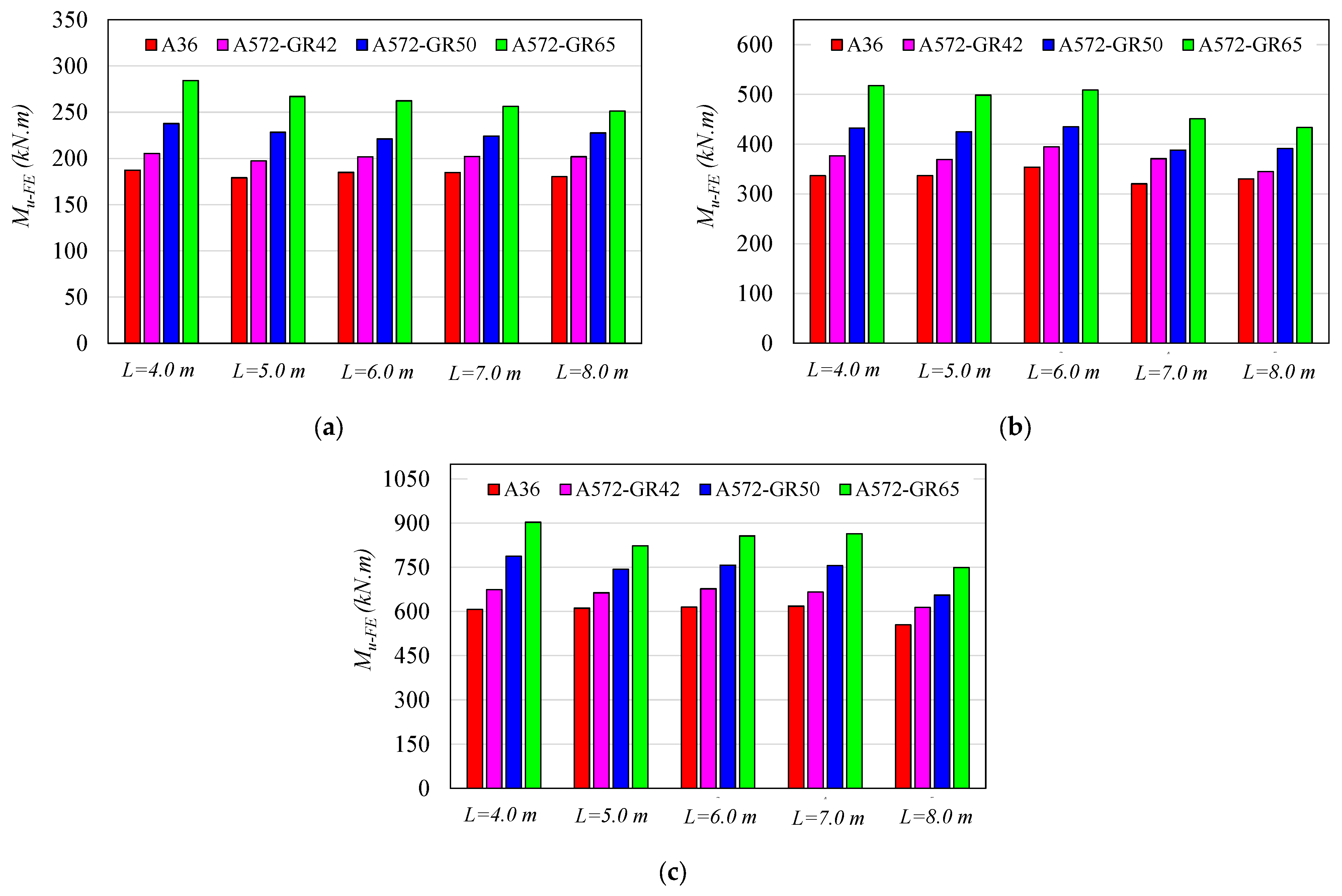
6.1. Steel Type Influence

In the parametric study developed, I-sections with mechanical properties of four different steel types were analyzed (Table 4). The ultimate moment results for models with the I-sections CB350, CB450, and CB600 are shown in Figure 14a–c, respectively. The results in Figure 14 are for models with longitudinal reinforcements with 8 mm diameter.

As expected, the highest LDB strengths were obtained for the steel A572 GR65, which has a yield strength (f_y) of 450 MPa. It is also observed that with the increase in the yield strength (f_y), there is an increase in the LDB ultimate moment. Taking as reference the steel with a yield strength of 250 MPa, it is verified that for an increase of 16%, 40%, and 80% in the yield strength (f_y = 290 MPa; f_y = 350 MPa; f_y = 450 MPa), the variation of the LDB ultimate moment was 10.12%, 23.60%, and 42.43%, respectively. Another fact that can be observed in Figure 14 is the small variation from the LDB ultimate moment due to the unrestricted length (L) variation, which shows that the span length is not a predominant factor in the LDB strength of SCCB.

For the development of a general analysis of the mechanical properties’ (f_y) influence of different steel types on the LDB strength of SCCB, Figure 15 is presented. In Figure 15, the reduction factor ($\chi =\frac{M_{u-FE}}{M_{pl-CB}}$) calculated as a function of the ultimate moment values obtained in the FE analyses, and, as a function of the composite section plastic moment, calculated according to the plastic theory (EC4 [13]), are compared for models with different steel types.

In Figure 15, the reference values for the reduction factor (χ_ref.) were calculated as a function of the ultimate moment values obtained for the steel A36 (f_y = 250 MPa). The results in Figure 15 show that the average value of the ratio (χ/χ_ref.) for the steel A572-GR65 is 0.86. This result is 14% lower when compared to the values obtained for the steel A36. This result shows that, although the LDB ultimate moment for A572-GR65 steel is higher than the value obtained with A36 steel, the value of the reduction factor (χ) is 14% lower. That is, for steels with a value of higher yield strength (f_y), there is a greater difficulty for the composite section to reach the plastic moment, with LDB being responsible for reducing the sectional moment. It is also observed in Figure 15 that the average value of the ratio (χ/χ_ref.) for A572-GR50 steel is 0.93, that is, 7% lower when compared to the values obtained for A36 steel. Finally, the reduction factor (χ) values for models with A572-GR42 steel are compared with the reference values. The average value of the ratio (χ/χ_ref.) for A572-GR42 steel is 0.98, that is, only 2% lower than the values of A36 steel. This proximity occurs due to the yield strength (f_y) of the two types of steels are close: 250 MPa for A36 steel and 290 MPa for A572-GR42 steel.

In order to compare the values of the reduction factor (χ), obtained through the FE analyses, with the values obtained through the standard procedures (ABNT NBR 8800:2008 [15] and EC4 [13]),

Table 5. Comparison between the reduction factor values (χ) calculated by standard procedures and obtained by FE analyses for models with 8 mm bars.

			fy = 250 MPa						fy = 290 MPa						fy = 350 MPa						fy = 450 MPa
			λ	χ			Percent Error (%)		λ	χ			Percent Error (%)		λ	χ			Percent Error (%)		λ	χ			Percent Error (%)
I-Section	ø (mm)	L (m)		FE	NBR	EC3	(χNBR − χFE)/χNBR	(χEC3 − χFE)/χEC3		FE	NBR	EC3	(χNBR − χFE)/χNBR	(χEC3 − χFE)/χEC3		FE	NBR	EC3	(χNBR − χFE)/χNBR	(χEC3 − χFE)/χEC3		FE	NBR	EC3	(χNBR − χFE)/χNBR	(χEC3 − χFE)/χEC3
CB350	8 mm	4	0.76	1.05	0.79	0.75	−33.8	−40.3	0.81	1.02	0.76	0.72	−33.7	−41.4	0.87	1.00	0.73	0.68	−38.1	−48.0	0.98	0.96	0.67	0.61	−43.2	−57.0
		5	0.76	1.01	0.78	0.75	−28.6	−34.9	0.81	0.98	0.76	0.72	−29.3	−36.8	0.88	0.96	0.72	0.67	−33.5	−43.2	0.98	0.90	0.67	0.61	−35.6	−49.0
		6	0.77	1.04	0.78	0.74	−33.1	−39.7	0.82	1.00	0.76	0.71	−32.4	−40.2	0.89	0.93	0.72	0.67	−29.6	−39.3	0.99	0.89	0.66	0.60	−33.8	−47.1
		7	0.77	1.04	0.78	0.74	−33.2	−39.9	0.82	1.00	0.75	0.71	−33.0	−40.9	0.89	0.95	0.72	0.67	−31.8	−41.6	0.99	0.87	0.66	0.60	−31.1	−44.3
		8	0.77	1.01	0.78	0.74	−30.0	−36.6	0.82	1.00	0.75	0.71	−32.9	−40.9	0.89	0.96	0.72	0.67	−34.0	−44.1	1.00	0.85	0.66	0.60	−28.7	−41.7
CB450	8 mm	4	0.81	1.00	0.76	0.72	−31.7	−39.3	0.86	0.98	0.73	0.68	−34.1	−43.3	0.94	0.95	0.69	0.64	−37.5	−49.5	1.06	0.90	0.63	0.56	−43.7	−60.4
		5	0.82	1.00	0.76	0.71	−32.8	−40.7	0.88	0.96	0.73	0.68	−32.5	−42.1	0.95	0.93	0.68	0.63	−36.6	−49.0	1.07	0.87	0.62	0.55	−40.3	−57.1
		6	0.83	1.05	0.75	0.71	−40.1	−48.7	0.88	1.03	0.72	0.67	−42.4	−52.9	0.96	0.96	0.68	0.62	−40.7	−53.7	1.08	0.89	0.61	0.55	−44.3	−61.8
		7	0.83	0.95	0.75	0.71	−27.2	−35.1	0.89	0.97	0.72	0.67	−34.4	−44.4	0.97	0.85	0.68	0.62	−25.9	−37.7	1.09	0.79	0.61	0.54	−28.6	−44.4
		8	0.83	0.98	0.75	0.70	−31.4	−39.6	0.89	0.90	0.72	0.67	−25.3	−34.7	0.97	0.86	0.67	0.62	−27.4	−39.4	1.09	0.76	0.61	0.54	−24.1	−39.4
CB600	8 mm	4	0.89	0.93	0.72	0.67	−28.9	−38.5	0.95	0.90	0.69	0.63	−30.9	−42.6	0.92	1.12	0.70	0.65	−59.2	−72.3	1.17	0.79	0.56	0.49	−40.5	−60.1
		5	0.90	0.93	0.71	0.66	−31.4	−41.7	0.97	0.88	0.68	0.62	−30.7	−43.0	0.94	1.06	0.69	0.64	−52.4	−65.6	1.19	0.72	0.55	0.48	−31.0	−49.8
		6	0.91	0.94	0.70	0.65	−33.3	−44.1	0.98	0.90	0.67	0.61	−34.6	−47.6	0.95	1.08	0.69	0.63	−56.6	−70.6	1.21	0.75	0.54	0.47	−38.2	−58.3
		7	0.92	0.94	0.70	0.65	−34.5	−45.6	0.99	0.89	0.67	0.61	−33.1	−46.3	0.95	1.07	0.68	0.63	−57.1	−71.4	1.21	0.76	0.54	0.47	−40.6	−61.2
		8	0.92	0.85	0.70	0.65	−21.1	−31.2	0.99	0.82	0.66	0.60	−23.1	−35.4	0.96	0.93	0.68	0.62	−36.7	−49.3	1.22	0.66	0.54	0.47	−22.7	−40.8
						Avg.	−31.4	−39.7				Avg.	−32.1	−42.2				Avg.	−39.8	−51.7				Avg.	−35.1	−51.5
						SD (%)	4.2	4.4				SD (%)	4.4	4.7				SD (%)	11.1	12.3				SD (%)	7.1	8.2
						Var. (%)	17.4	19.1				Var. (%)	19.0	21.8				Var. (%)	124.1	152.2				Var. (%)	51.1	67.9

,

Table 6. Comparison between the reduction factor values (χ) calculated by standard procedures and obtained by FE analyses for models with 16 mm bars.

			fy = 250 MPa						fy = 290 MPa						fy = 350 MPa						fy = 450 MPa
			λ	χ			Percent Error (%)		λ	χ			Percent Error (%)		λ	χ			Percent Error (%)		λ	χ			Percent Error (%)
I-Section	ø (mm)	L (m)		FE	NBR	EC3	(χNBR − χFE)/χNBR	(χEC3 − χFE)/χEC3		FE	NBR	EC3	(χNBR − χFE)/χNBR	(χEC3 − χFE)/χEC3		FE	NBR	EC3	(χNBR − χFE)/χNBR	(χEC3 − χFE)/χEC3		FE	NBR	EC3	(χNBR − χFE)/χNBR	(χEC3 − χFE)/χEC3
CB350	16 mm	4	0.62	0.82	0.85	0.83	3.3	0.4	0.66	0.81	0.83	0.81	2.8	−0.5	0.71	0.77	0.81	0.78	5.3	1.5	0.78	0.75	0.78	0.74	2.8	−2.2
		5	0.63	0.81	0.85	0.82	4.7	1.8	0.66	0.77	0.83	0.80	7.2	4.0	0.71	0.72	0.81	0.78	10.4	6.7	0.78	0.72	0.77	0.73	6.2	1.2
		6	0.63	0.80	0.85	0.82	6.1	3.2	0.67	0.78	0.83	0.80	5.6	2.3	0.72	0.74	0.81	0.77	8.7	4.9	0.79	0.72	0.77	0.73	7.1	2.1
		7	0.63	0.79	0.85	0.82	7.0	4.2	0.67	0.75	0.83	0.80	9.9	6.7	0.72	0.75	0.81	0.77	6.5	2.6	0.79	0.72	0.77	0.73	6.2	1.1
		8	0.63	0.79	0.85	0.82	6.6	3.7	0.67	0.77	0.83	0.80	6.8	3.5	0.72	0.73	0.80	0.77	9.6	5.8	0.79	0.68	0.77	0.73	12.2	7.4
CB450	16 mm	4	0.69	0.83	0.82	0.79	−0.7	−4.5	0.73	0.80	0.80	0.77	0.4	−3.9	0.78	0.81	0.77	0.74	−4.2	−9.7	0.87	0.79	0.73	0.68	−8.2	−15.7
		5	0.69	0.80	0.82	0.79	1.6	−2.2	0.74	0.80	0.80	0.76	−0.6	−5.1	0.79	0.78	0.77	0.73	−1.4	−6.9	0.88	0.74	0.72	0.68	−2.6	−10.1
		6	0.70	0.83	0.81	0.78	−2.0	−6.0	0.74	0.83	0.79	0.76	−4.6	−9.4	0.80	0.80	0.77	0.73	−5.1	−11.0	0.88	0.75	0.72	0.67	−4.7	−12.4
		7	0.70	0.80	0.81	0.78	2.2	−1.7	0.75	0.76	0.79	0.76	4.3	−0.2	0.80	0.76	0.76	0.72	0.9	−4.6	0.89	0.69	0.72	0.67	3.6	−3.6
		8	0.71	0.79	0.81	0.78	3.3	−0.6	0.75	0.76	0.79	0.76	4.2	−0.3	0.80	0.72	0.76	0.72	5.3	−0.1	0.89	0.67	0.72	0.67	6.3	−0.8
CB600	16 mm	4	0.78	0.79	0.78	0.74	−1.6	−6.9	0.82	0.79	0.76	0.71	−5.0	−11.2	0.89	0.78	0.72	0.67	−7.6	−15.6	0.99	0.73	0.67	0.61	−9.1	−19.8
		5	0.79	0.79	0.77	0.73	−3.0	−8.7	0.83	0.79	0.75	0.70	−5.8	−12.4	0.90	0.76	0.71	0.66	−6.1	−14.3	1.00	0.70	0.66	0.60	−6.4	−17.3
		6	0.80	0.81	0.76	0.72	−5.9	−11.9	0.84	0.80	0.74	0.70	−8.2	−15.2	0.91	0.76	0.71	0.65	−7.5	−16.1	1.01	0.69	0.65	0.59	−6.2	−17.4
		7	0.81	0.80	0.76	0.72	−5.4	−11.4	0.85	0.82	0.74	0.70	−10.0	−17.3	0.92	0.73	0.70	0.65	−3.9	−12.3	1.02	0.68	0.65	0.58	−5.3	−16.5
		8	0.81	0.73	0.76	0.72	3.6	−2.0	0.85	0.73	0.74	0.69	1.7	−4.8	0.92	0.68	0.70	0.65	3.1	−4.9	1.02	0.61	0.64	0.58	5.8	−4.3
						Avg.	1.3	−2.8				Avg.	0.6	−4.2				Avg.	0.9	−4.9				Avg.	0.5	−7.2
						SD (%)	4.2	5.3				SD (%)	6.1	7.4				SD (%)	6.5	8.1				SD (%)	6.8	8.8
						Var. (%)	17.7	27.6				Var. (%)	37.0	55.0				Var. (%)	41.8	65.2				Var. (%)	46.4	77.5

and

Table 7. Comparison between the reduction factor values (χ) calculated by standard procedures and obtained by FE analyses for models with 25 mm bars.

			fy = 250 MPa						fy = 290 MPa						fy = 350 MPa						fy = 450 MPa
			λ	χ			Percent Error (%)		λ	χ			Percent Error (%)		λ	χ			Percent Error (%)		λ	χ			Percent Error (%)
I-Section	ø (mm)	L (m)		FE	NBR	EC3	(χNBR − χFE)/χNBR	(χEC3 − χFE)/χEC3		FE	NBR	EC3	(χNBR − χFE)/χNBR	(χEC3 − χFE)/χEC3		FE	NBR	EC3	(χNBR − χFE)/χNBR	(χEC3 − χFE)/χEC3		FE	NBR	EC3	(χNBR − χFE)/χNBR	(χEC3 − χFE)/χEC3
CB350	25 mm	4	0.48	0.81	0.91	0.89	10.5	9.0	0.50	0.81	0.90	0.88	10.5	8.8	0.56	0.72	0.88	0.86	18.0	16.0	0.64	0.67	0.84	0.82	20.6	18.1
		5	0.49	0.79	0.91	0.89	13.2	11.7	0.50	0.77	0.90	0.88	14.3	12.7	0.57	0.70	0.87	0.85	20.3	18.3	0.65	0.64	0.84	0.81	24.2	21.7
		6	0.49	0.76	0.91	0.89	16.2	14.7	0.51	0.81	0.90	0.88	10.0	8.3	0.57	0.71	0.87	0.85	18.9	16.9	0.65	0.62	0.84	0.81	25.5	23.0
		7	0.49	0.78	0.90	0.89	14.3	12.8	0.51	0.79	0.90	0.88	11.6	9.9	0.57	0.70	0.87	0.85	19.9	17.9	0.65	0.62	0.84	0.81	26.1	23.6
		8	0.49	0.78	0.90	0.89	13.6	12.1	0.51	0.79	0.90	0.88	12.4	10.7	0.57	0.69	0.87	0.85	20.4	18.4	0.65	0.61	0.84	0.81	27.2	24.7
CB450	25 mm	4	0.57	0.74	0.87	0.85	15.0	12.9	0.61	0.70	0.86	0.83	17.9	15.6	0.66	0.69	0.83	0.81	16.8	13.9	0.73	0.67	0.80	0.76	16.1	12.4
		5	0.57	0.72	0.87	0.85	17.2	15.1	0.62	0.69	0.85	0.83	18.9	16.5	0.67	0.67	0.83	0.80	18.6	15.8	0.74	0.66	0.79	0.76	16.9	13.1
		6	0.58	0.79	0.87	0.85	9.6	7.3	0.62	0.74	0.85	0.83	13.4	10.9	0.68	0.69	0.83	0.80	16.3	13.3	0.75	0.66	0.79	0.76	16.7	12.8
		7	0.58	0.72	0.87	0.85	17.4	15.3	0.62	0.67	0.85	0.83	20.9	18.5	0.68	0.65	0.82	0.80	21.3	18.4	0.75	0.60	0.79	0.75	23.9	20.3
		8	0.58	0.71	0.87	0.85	17.8	15.7	0.63	0.66	0.85	0.82	22.2	19.9	0.68	0.63	0.82	0.79	23.9	21.2	0.75	0.57	0.79	0.75	27.7	24.3
CB600	25 mm	4	0.67	0.69	0.83	0.80	16.9	14.0	0.71	0.69	0.81	0.78	15.0	11.5	0.77	0.66	0.78	0.75	15.4	11.1	0.85	0.64	0.74	0.70	13.9	8.3
		5	0.68	0.70	0.82	0.79	14.9	11.8	0.72	0.69	0.80	0.77	14.6	11.0	0.78	0.66	0.78	0.74	15.3	10.8	0.86	0.63	0.73	0.69	14.8	8.9
		6	0.69	0.73	0.82	0.79	11.6	8.3	0.73	0.71	0.80	0.77	11.5	7.6	0.79	0.68	0.77	0.73	12.4	7.7	0.87	0.61	0.73	0.68	15.9	9.9
		7	0.69	0.73	0.82	0.79	11.3	7.9	0.73	0.70	0.80	0.76	12.0	8.0	0.79	0.67	0.77	0.73	12.6	7.8	0.87	0.62	0.73	0.68	14.6	8.5
		8	0.69	0.66	0.82	0.79	19.4	16.3	0.74	0.64	0.80	0.76	19.0	15.4	0.80	0.59	0.77	0.73	23.4	19.2	0.88	0.56	0.72	0.68	23.2	17.6
						Avg.	14.6	12.3				Avg.	14.9	12.3				Avg.	18.2	15.1				Avg.	20.5	16.5
						SD (%)	2.9	3.0				SD (%)	3.9	3.9				SD (%)	3.5	4.2				SD (%)	5.1	6.2
						Var. (%)	8.6	9.0				Var. (%)	15.3	15.3				Var. (%)	12.1	17.4				Var. (%)	26.0	38.7

are shown. In standard procedures, the reduction factor (χ) is obtained as a function of the relative slenderness factor ($\lambda =\sqrt{\frac{M_{cr}}{M_{pl-CB}}}$) calculated as a function of the LDB elastic critical moment and the plastic moment of the composite section, which is dependent on the steel yield strength (f_y).

Table 5 presents the results for the models with 8 mm reinforcement bars, comparisons are made between the values of the reduction factor (χ) obtained by the standard procedures and through the FE analyses for each type of steel used in the I-sections. In Table 6 and Table 7 the same comparisons are made, however, for models with 16 mm and 25 mm reinforcement bars, respectively. More information about the results obtained for each beam can be found on Appendix A.

It is observed in Table 5 that the values of the reduction factor (χ) obtained by the standard procedures (NBR 8800:2008 [15] and EC4 [13]) are lower than the values obtained with the FE analyses. This situation shows a very conservative behavior of the Brazilian [15], for models with 8 mm reinforcement bars, a situation also observed by Rossi et al. [1], Zhou and Yan [4], and Bradford [29], in relation to the European procedure [13]. Table 5 also presents the percentage error values of the standard procedures calculated in relation to the results obtained with the FE analyses. Percentage error values were calculated for models with different steel types. For the Brazilian standard procedure [15], the average values of the percentage error for steels with a yield strength (f_y) of 250 MPa, 290 Mpa, 350 Mpa, and 450 MPa were −31.4%, −32.1%, −39.8%, and −35.1%, respectively. These results show that the LDB ultimate moment values obtained by the Brazilian standard procedure [15] are inferior to the values obtained by the FE analyses, verifying a considerably conservative situation. When the results are compared with the values obtained by the European standard procedure [13], there is an intensification of this conservative situation. The percentage error values for the European standard [13] are −39.7%, −42.2%, −51.7%, and −51.5% for steels with a yield strength of 250 MPa, 290 MPa, 350 MPa, and 450 MPa, respectively. Therefore, the ultimate moment values obtained by the European procedure [13] are up to 50% lower than the values obtained with the FE analyses for the models with reinforcement bars of 8mm.

Still in relation to Table 5, observing the percentage error evolution for the different steel types, a growth tendency of the errors is verified with the yield strength (f_y) increase, except for the steel with a yield strength of 450 MPa. This situation shows that the use of steels with different mechanical characteristics has an impact on the LDB strength that is not captured by the design curves of SSRC (used by NBR 8800:2008 [15]) and ECCS (used by EC3), which use the relative slenderness factor ($\lambda =\sqrt{\frac{M_{cr}}{M_{pl-CB}}}$).

Table 6 presents the results for models with 16 mm reinforcement bars. The results of Table 6 show a greater proximity between the LDB ultimate moment values obtained by the standard procedures and by the FE analyses. This situation can be explained by the plastic moment calculation of the composite section, which is dependent on the longitudinal reinforcement area present in the effective width of the concrete slab. Therefore, with the increase in the steel area, there is an increase in the plastic moment, and, therefore, a reduction in the relative slenderness factor ($\lambda =\sqrt{\frac{M_{cr}}{M_{pl-CB}}}$), and, consequently, an increase in the reduction factor (χ). Thus, with the increase in the plastic moment and the reduction factor, there is an increase in the value of the LDB ultimate moment, which leads to a closer approximation with the standard values. It is observed in Table 6 that the average values of the percentage error for the Brazilian standard [15] are 1.3%, 0.6%, 0.9%, and 0.5%, and for the European standard [13] −2.8%, −4.2%, −4.9%, and −7.2%, for steels with a yield strength of 250 MPa, 290 MPa, 350 MPa, and 450 MPa, respectively. Regarding the steel type, it is verified, for the Brazilian procedure [15] (curve 2P of the SSRC), that there is no great variation in the average values of the percentage errors for the different steel types. However, for the European standard [13], there is an increase in divergences with the increase in the I-section steel yield strength.

Finally, Table 7 shows the results for models with reinforced bars with 25 mm diameter. Contrary to the results observed in Table 5, Table 7 shows a non-conservative situation of the standard procedures; that is, the results of the FE analyses were lower than the ultimate moment values obtained by the standard procedures. The explanation for this situation is the same as that presented in the previous paragraph; that is, with the increase of the steel area in the effective width of the concrete slab, there is an increase in the plastic moment, and, therefore, a reduction in the relative slenderness factor ($\lambda =\sqrt{\frac{M_{cr}}{M_{pl-CB}}}$), and, consequently, an increase in the reduction factor (χ). Thus, with the increase in the plastic moment and the reduction factor, there is an increase in the LDB ultimate moment value, higher than those obtained in the FE analyses. In Table 7, it is observed that the average values of the percentage error in relation to the Brazilian standard [15] are 14.6%, 14.9%, 18.2%, and 20.5%, for the European standard [13] these values are 12.3%, 12.3%, 15.1%, and 16.5%, for steels with a yield strength of 250 MPa, 290 MPa, 350 MPa, and 450 MPa, respectively. Analyzing the percentage error evolution, it is also observed a small influence of the yield strength variation on the LDB ultimate moment values that are not captured by the classic SSRC and ECCS curves.

Figure 16 shows the deformed shape and von Mises stresses, for the CB450 model with a length of 6.0 m and reinforcement bars with 8 mm diameter for the four steel types analyzed. For the model with steel yield strength of 250 MPa (Figure 16a), the maximum stress in the I-section web (middle of the span) varies from 230.30 to 258.98 MPa. For the model with 290 MPa yield strength (Figure 16b), the maximum stress in the I-section web varies from 287.60 to 316.31 MPa. For the model in Figure 16c, with a yield strength of 350 MPa, the maximum web stress ranges from 332.94 to 363.16 MPa, and finally, for the model with a yield strength of 450 MPa (Figure 16d) the maximum web stress varies from 422.35 to 460.67 MPa.

6.2. Analytical Procedures and Other Parameters

The increase in the area of reinforcement bars present in the effective width of the concrete slab causes the increase in the plastic moment of the composite section calculated by plastic theory, which consequently leads to an increase in the LDB ultimate moment calculated by standard procedures such as EC4 [13] and NBR 8800:2008 [15]. However, the numerical analyses developed in this article show a small variation in LDB strength due to the increase in the area of reinforcement bars. 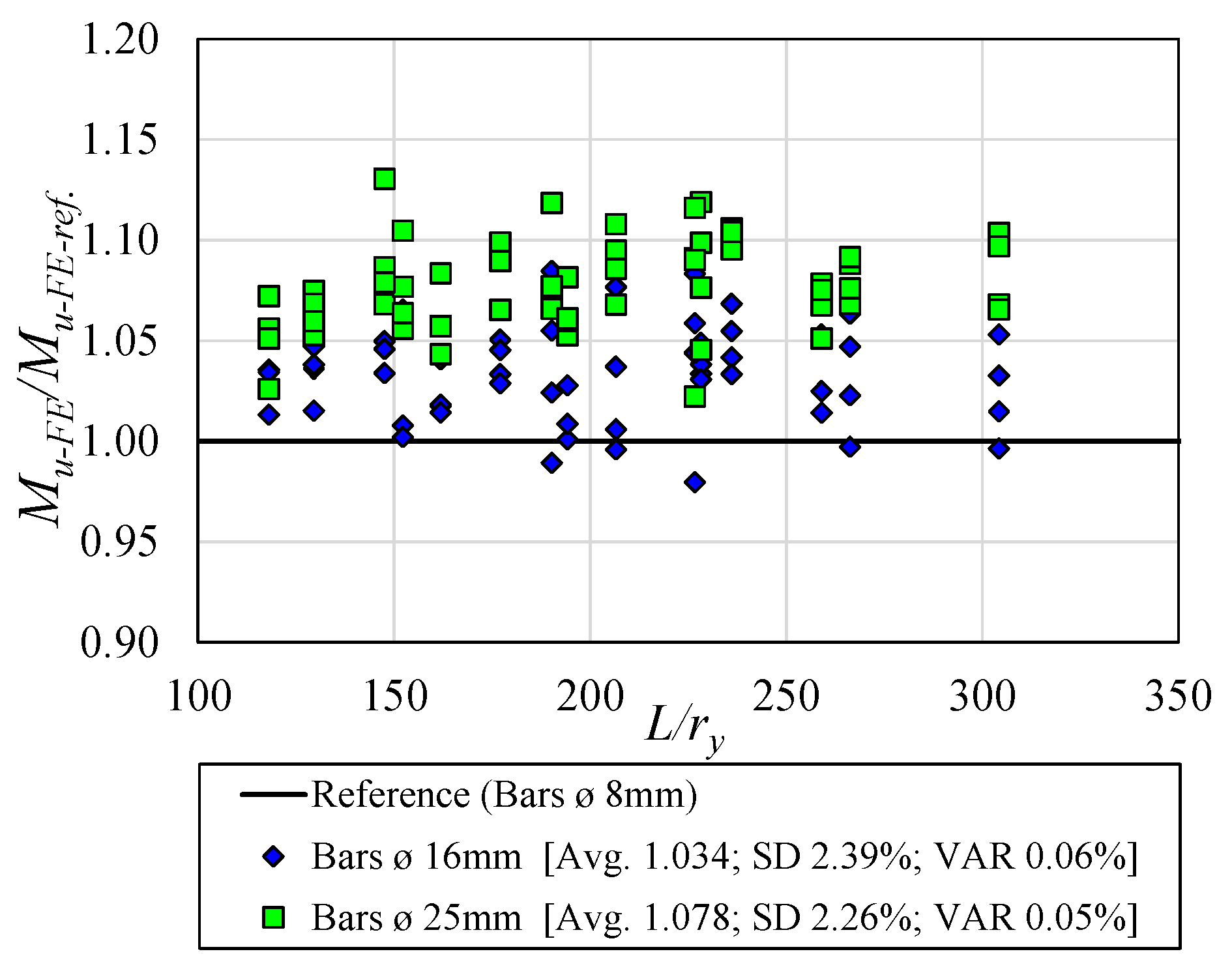Figure 17 shows the LDB ultimate moment results for models with reinforcement bars with a diameter of 8 mm, 16 mm, and 25 mm. In Figure 17 the reference values are those obtained by the models with 8 mm bars.

It is observed in Figure 17 that the average value of the ratio (M_u-FE/M_u-FE-ref.) for models with reinforcement bars with 16 mm diameter is 1.034; that is, there is an average gain in the ultimate moment value of about 3.4%. Regarding the models with 25 mm bars, the average value of the ratio (M_u-FE/M_u-FE-ref.) is 1.078. This shows that the ultimate moment has an average gain of 7.8% compared with the models with 8 mm bars. This situation shows that, despite a considerable increase in the longitudinal reinforcement area, there is an insignificant increase in the value of the LDB ultimate moment.

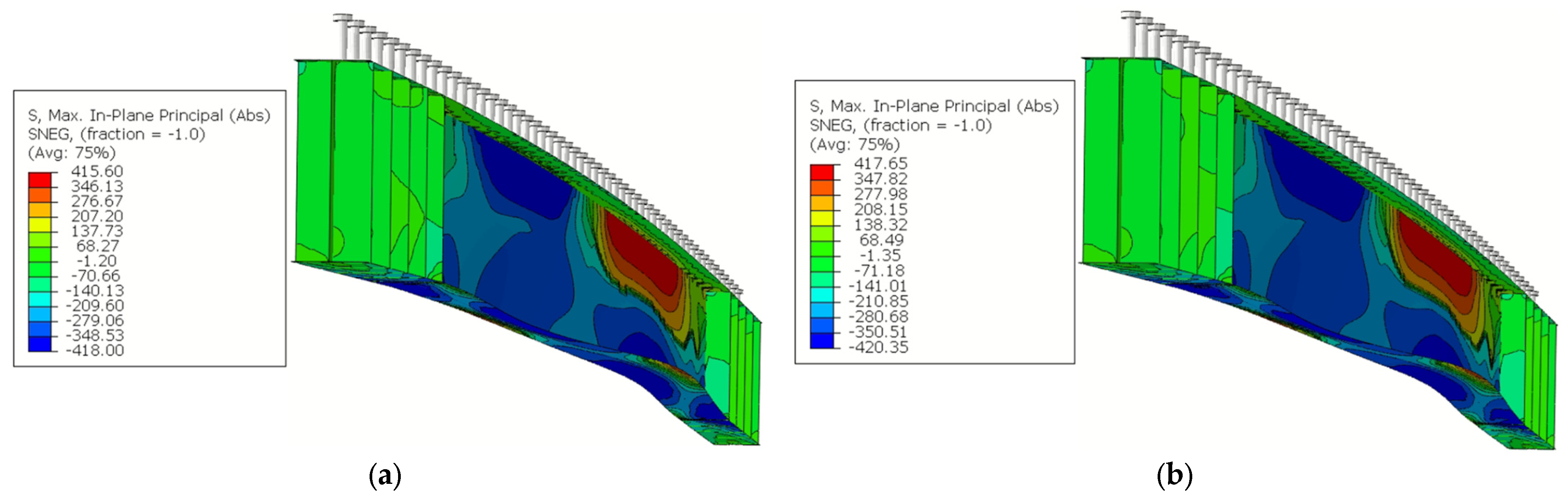
Figure 18 shows the deformed shape and the distribution of the absolute maximum stresses in the principal plane for models CB350 with a length of 6.0 m, A572-GR50 steel and with longitudinal reinforcements of 8 mm (Figure 18a), 16 mm (Figure 18b), and 25 mm (Figure 18c). It is observed in Figure 18 that the increase in the longitudinal reinforcement area in the effective width of the concrete slab causes an increase in the maximum tension and compression stresses, reflecting the increase in the LDB ultimate moment, a situation verified in the numerical models analyzed.

As seen in Figure 17, the increase in the longitudinal reinforcement area in the effective width of the concrete slab leads to an insignificant increase in the LDB ultimate moment. However, this increase in the longitudinal reinforcement area causes a considerable increase in the plastic moment value calculated according to EC4 [13] by plastic theory. This situation causes an increase in the LDB ultimate moment value, calculated according to the procedures of EC4 [13] and NBR 8800:2008 [15], as the longitudinal reinforcement area increases. 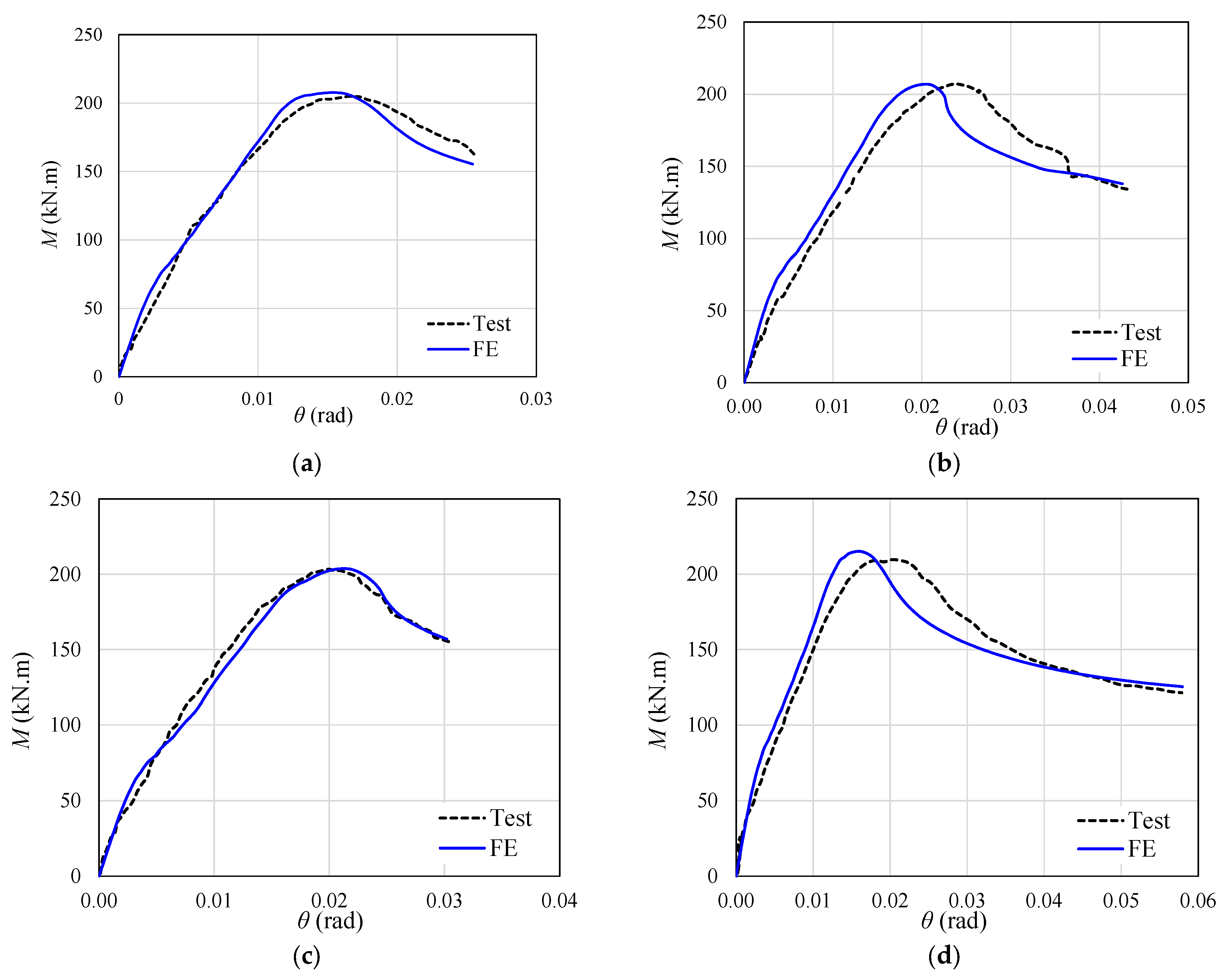Figure 19 shows the comparison between the European [13] and Brazilian [15] standard design curves with the results of the FE analyses for models with 8 mm (Figure 19a), 16 mm (Figure 19b), and 25 mm (Figure 19c). In addition, Figure 19 also shows the values of the experimental analysis of four beams tested by Tong et al. [28], which served to validate the numerical model of this article.

It is observed in Figure 19 three different situations. In Figure 19a, the results of the FE analyses provided LDB ultimate moment values higher than those obtained by the Brazilian [15] and European [13] standard procedures. The average percentage error of the FE analyses results when compared to the European procedure [13] was −46.28%, which shows considerable conservatism in the EC4 procedure [13]. Regarding the Brazilian standard [15], which is based on the SSRC 2P curve, the average percentage error was −34.60%, also showing conservatism. Figure 19a also presents the results of four beams tested experimentally by Tong et al. [28]. The results of these four beams are close to the values of the FE analyses developed in this article, since the longitudinal reinforcement area of the beams by Tong et al. [28] is similar to the models with 8 mm bars analyzed in the present work.

In relation to Figure 19b, which presents the results for the models with 16 mm diameter longitudinal reinforcement, a close proximity is observed between the results of the FE analyses and the standard procedures of EC4 [13] and NBR 8800:2008 [15]. The increase in the plastic moment of the composite section is the reason that leads to the greater proximity between the results of the standard procedures and those obtained through the FE analyses. For the results presented in Figure 19b, the average percentage error of the numerical results compared with the standard procedures is 0.83% for the Brazilian standard [15] and −4.78% for the European standard [13]. Finally, in Figure 19c, the results of the FE analyses are compared with the standard procedures for the models with 25 mm diameter longitudinal reinforcement. It is observed in Figure 19c that the LDB ultimate moment values obtained by means of the FE analyses are inferior to the standard results, which leads to an unsafe situation of the European [13] and Brazilian [15] standards. As verified, the increase in the longitudinal reinforcement area does not cause a considerable gain in the LDB strength. However, for the EC4 [13] and NBR 8800:2008 [15] procedures, the increase in the longitudinal reinforcement area leads to a considerable gain from the LDB strength of SCCB, which leads to this unsafe situation for the European [13] and Brazilian [15] procedures. In Figure 19c the average percentage error of the numerical results compared with the standard procedures is 17.05% for the Brazilian standard [15] and 14.05% for the European standard [13].

The results of the FE analyses were also compared with the analytical procedures presented by Zhou and Yan [4] and Bradford [29]. In Figure 20, the results of the FE analyses are compared with the Zhou and Yan procedure [4].

It is observed in Figure 20 that the longitudinal reinforcement area variation in the concrete slab is also responsible for three different situations when the results of the FE analyses are compared with the Zhou and Yan procedure [4]. For the models with 8 mm diameter longitudinal reinforcement (Figure 20a) the results of the FE analyses show greater agreement with the Zhou and Yan [4] procedure. The results analysis of the LDB ultimate moment shows that the average value of the ratio (M_{Zhou and Yan}/M_u,_FE) is 1.08, that is, the values obtained through the analytical procedure of Zhou and Yan [4] are on average 8.0% higher than those obtained with the FE analyses. Figure 20b presents the results obtained with the FE analyses for the models with 16 mm bars. It is verified that with the increase in the longitudinal reinforcement area there is also an increase in the divergence between the results of the FE analyses and the results of the Zhou and Yan procedure [4]. The average value of the ratio (M_{Zhou and Yan}/M_u,_FE) is 1.28, that is, the results of the procedure developed by the authors [4] are on average 28% higher than the results obtained in the numerical analysis, an unsafe situation. Finally, Figure 20c shows the results for the models with 25 mm diameter longitudinal reinforcement bars. There is also a tendency to increase the divergence between the numerical results and the Zhou and Yan [4] procedure as the longitudinal reinforcement area is increased. For the results in Figure 20c, the average value of the ratio (M_{Zhou and Yan}/M_u,_FE) is 1.34, which shows an unsafe situation in the Zhou and Yan procedure [4]. Figure 20 also presents the results for the models with the different steel types analyzed, it is verified that, as for the standard procedures, in the Zhou and Yan procedure [4] the influence of the steel type is not captured properly.

Finally, Figure 21 presents the comparison between the results obtained with the FE analyses and the Bradford [29] procedure.

The results in Figure 21 show a similar behavior of the Bradford procedure [29] in comparison with the results of the FE analysis between the models with longitudinal reinforcement of 8 mm (Figure 21a), 16 mm (Figure 21b), and 25 mm (Figure 21c). This situation is due to the fact that the Bradford procedure [29] does not consider the plastic moment of the composite section, but only the I-section plastic moment to determine the LDB ultimate moment. This situation can be confirmed with the analysis of the average value of the ratio (M_Bradford/M_u,_FE) which provided values of 0.59, 0.57, and 0.55 for the models with reinforcement bars with a diameter of 8 mm, 16 mm, and 25 mm, respectively. However, despite providing safe results, the Bradford procedure [29] is considerably conservative. Regarding the results for the different steel types analyzed, it is verified that for the models with greater steel yield strength, there is a greater proximity of the FE results with the author’s procedure [29]. On the other hand, with the reduction in the steel yield strength, there is a tendency to increase the divergences between the FE results and the Bradford procedure [29].

Finally, Figure 22 shows the LDB ultimate moment values for models with A572-GR50 steel and 8 mm reinforcement bars. The results show that the unrestricted length variation does not significantly influence the LDB ultimate moment value, a situation also observed by Rossi et al. [1]. It is verified in Figure 22 that the preponderant factor in the LDB ultimate moment values is the I-section geometric properties.

The results presented show that the standard procedures are still flawed in determining the LDB strength of SCCB under the action of the hogging moment. The influence of parameters not previously investigated was presented, such as the I-section steel type and a considerable variation in the longitudinal reinforcement area in the effective width of the concrete slab. The investigation of these factors showed flaws until then not observed, in the standard procedures such as EC4 [13] and NBR8800:2008 [15]. The comparison between the FE results and the analytical procedures, such as Zhou and Yan [4] and Bradford [29], shows that further investigations are still needed to fully understand the LDB phenomenon in SCCB. Thus, the results presented in this article can provide a reference for future research and specification reviews.

7. Conclusions

In this article, the LDB strength of SCCB was investigated through the development of post-buckling numerical analyses with the ABAQUS software. The SCCB analyzed are simply supported with lateral bracing. In the parametric study, 180 analyses were developed, varying the following factors: the mechanical properties of the steel I-section, the dimensions of the I-sections, the unrestricted length, and the longitudinal reinforcement area present in the effective width of the concrete slab. Finally, the results were compared with current standard procedures and analytical proposals. In this way, it was concluded:

• The increase in the I-section steel yield strength causes an increase in the LDB ultimate moment values. Taking as reference the steel with a yield strength of 250 MPa, it is verified that for an increase of 16%, 40%, and 80% in the yield strength (f_y = 290; f_y = 350; f_y = 450), the variation in the LDB ultimate moment was of 10.12%, 23.60%, and 42.43%, respectively.
• It was verified that for the models with a higher steel yield strength (f_y), the LDB occurs for ultimate moment values lower than the plastic moment of the composite section, that is, the greater the steel yield strength, the lower the chances of the composite section reaching the plastic moment, with the LDB being the failure mode responsible for defining the ultimate moment value;
• There was a tendency to increase divergences between the numerical results and the curves of ECCS (EC4) and SSRC (NBR 8800:2008), with the increase in the steel yield strength (f_y), that is, for steels with greater yield strength, the greater the divergences between the FE results and standard procedures.
• The increase in the longitudinal reinforcement area present in the concrete slab causes a small increase in the LDB strength. For an increase of 244% in the longitudinal reinforcement area, there was only an increase of about 7.8% in the value of the LDB ultimate moment;
• Different behavior of the standard procedures was verified, due to the variation of the longitudinal reinforcement area, when compared to the ultimate moment obtained by the FE analyses. For a longitudinal reinforcement rate that approximates practical situations (8 mm bars), the standard procedures proved to be considerably conservative. As the longitudinal reinforcement area in the effective width of the concrete slab is increased, the behavior of the standard procedures is changed. For the longitudinal reinforcement with 16 mm bars, the standard results are close to the numerical values, showing a good behavior of the standard procedures. However, for models with 25 mm bars, the European [13] and Brazilian [15] standard procedures provided ultimate moment results superior to those obtained by FE analyses;
• The Zhou and Yan [4] procedure showed a behavior similar to that observed in the standard procedures, that is, with the increase in the longitudinal reinforcement rate, there is a variation of the divergences with the results of the FE analyses. This situation is caused by the fact that the procedures of Zhou and Yan [4], the European standard [13] and the Brazilian standard [15], define the LDB ultimate moment value due to the reduction of the plastic moment of the composite section, and, any change in this value was shown to be sensitive to the behavior of the mentioned procedures;
• It was found that the Bradford procedure [29] is not sensitive to the variation in the longitudinal reinforcement rate, since the definition of the LDB ultimate moment is a function of the I-section plastic moment, and not of the composite section plastic moment. The comparison between the results of the FE analyses and Bradford’s procedure [29] showed that this provides safe results, however, considerably conservative;
• It was verified that the LDB ultimate moment is not very sensitive to the unrestricted length variation of the SCCB. The predominant factor is the dimensions of the I-section.

In general, it was verified that the standard procedures are still flawed in determining the LDB strength of SCCB. It was found that the European [13] and the Brazilian [15] standard procedures show different behaviors due to the longitudinal reinforcement area variation. In addition, they are sensitive to the variation of the steel mechanical properties, tending to an increase or reduction of the divergences depending on the yield strength variation (f_y). The comparison between the FE results and the analytical procedures, such as Zhou and Yan [4] and Bradford [29], shows that further investigations are still needed to fully understand the LDB phenomenon in SCCB. Thus, the results presented in this article can provide a reference for future research and specification reviews.

References

1. Rossi, A.; Nicoletti, R.S.; de Souza, A.S.C.; Martins, C.H. Numerical Assessment of Lateral Distortional Buckling in Steel-Concrete Composite Beams. J. Constr. Steel Res. 2020, 172, 106192. [Google Scholar] [CrossRef]
2. Vrcelj, Z.; Bradford, M.A. Inelastic Restrained Distortional Buckling of Continuous Composite T-Beams. J. Constr. Steel Res. 2009, 65, 850–859. [Google Scholar] [CrossRef]
3. Rossi, A.; Nicoletti, R.S.; de Souza, A.S.C.; Martins, C.H. Lateral Distortional Buckling in Steel-Concrete Composite Beams: A Review. Structures 2020, 27, 1299–1312. [Google Scholar] [CrossRef]
4. Zhou, W.-B.; Yan, W.-J. Refined Nonlinear Finite Element Modelling towards Ultimate Bending Moment Calculation for Concrete Composite Beams under Negative Moment. Thin-Walled Struct. 2017, 116, 201–211. [Google Scholar] [CrossRef]
5. Moghbeli, A.; Sharifi, Y. New Predictive Equations for Lateral-Distortional Buckling Capacity Assessment of Cellular Steel Beams. Structures 2021, 29, 911–923. [Google Scholar] [CrossRef]
6. Hosseinpour, M.; Sharifi, Y.; Sharifi, H. Neural Network Application for Distortional Buckling Capacity Assessment of Castellated Steel Beams. Structures 2020, 27, 1174–1183. [Google Scholar] [CrossRef]
7. Dietrich, M.Z.; Calenzani, A.F.G.; Fakury, R.H. Analysis of Rotational Stiffness of Steel-Concrete Composite Beams for Lateral-Torsional Buckling. Eng. Struct. 2019, 198, 109554. [Google Scholar] [CrossRef]
8. Chen, S.; Wang, X. Finite Element Analysis of Distortional Lateral Buckling of Continuous Composite Beams with Transverse Web Stiffeners. Adv. Struct. Eng. 2012, 15, 1607–1616. [Google Scholar] [CrossRef]
9. Yang, L.; Lewei, T.; Bo, S.; Yiyi, C.; Feng, Z.; Tian Hal, S.X. FEA and Bending Capacity Calculation for Mechanical Behavior of Steel-Concrete Composite Beams under Negative Bending. J. Build. Struct. 2014, 35, 10–21. [Google Scholar]
10. Vasdravellis, G.; Uy, B.; Tan, E.L.; Kirkland, B. The Effects of Axial Tension on the Hogging-Moment Regions of Composite Beams. J. Constr. Steel Res. 2012, 68, 20–33. [Google Scholar] [CrossRef]
11. Chen, S.; Jia, Y. Numerical Investigation of Inelastic Buckling of Steel–Concrete Composite Beams Prestressed with External Tendons. Thin-Walled Struct. 2010, 48, 233–242. [Google Scholar] [CrossRef]
12. Bradford, M.; Johnson, R. Inelastic Buckling of Composite Bridge Girders Near Internal Supports. Proc. Inst. Civ. Eng. 1987, 83, 143–159. [Google Scholar] [CrossRef]
13. EN 1994-1-1; Eurocode 4: Design of Composite Steel and Concrete Structures—Part 1-1: General Rules and Rules for Buildings. Standard. Comite Europeen de Normalisation: Brussels, Belgium, 2004.
14. Roik, K.; Hanswille, G.; Kina, J. Solution for the Lateral Torsional Buckling Prob Lem of Composite Beams. Stahlbau 1990, 59, 327–332. (In German) [Google Scholar]
15. ABNT NBR 8800; Projeto de Estruturas de Aço e de Estruturas Mistas de Aço e Concreto de Edifícios, Standard. Associação Brasileira de Normas Técnicas: Rio de Janeiro, Brazil, 2008.
16. ANSI/AISC 360-16; ANST/AISC AISC 360-16: Specification for Structural Steel Buildings. ANSI: Washington, DC, USA, 2016; Volume 676.
17. AS 4100; Steel Structures. Standards Association of Australia: Sydney, Australia.
18. Dias, J.V.F.; Oliveira, J.P.S.; Calenzani, A.F.G.; Fakury, R.H. Elastic Critical Moment of Lateral-Distortional Buckling of Steel-Concrete Composite Beams under Uniform Hogging Moment. Int. J. Struct. Stab. Dyn. 2019, 19, 1950079. [Google Scholar] [CrossRef]
19. Zhou, W.B.; Jiang, L.Z.; Li, S.J.; Kong, F. Elastic Distortional Buckling Analysis of I-Steel Concrete Composite Beam Considering Shear Deformation. Int. J. Struct. Stab. Dyn. 2016, 16, 1–22. [Google Scholar] [CrossRef]
20. Ye, J.H.; Chen, W. Elastic Restrained Distortional Buckling of Steel-Concrete Composite Beams Based on Elastically Supported Column Method. Int. J. Struct. Stab. Dyn. 2013, 13, 1–29. [Google Scholar] [CrossRef]
21. Svensson, S.E. Lateral Buckling of Beams Analysed as Elastically Supported Columns Subject to a Varying Axial Force. J. Constr. Steel Res. 1985, 5, 179–193. [Google Scholar] [CrossRef]
22. Williams, F.W.; Jemah, A.K. Buckling Curves for Elastically Supported Columns with Varying Axial Force, to Predict Lateral Buckling of Beams. J. Constr. Steel Res. 1987, 7, 133–147. [Google Scholar] [CrossRef]
23. Hanswille, G.; Lindner, J.; Munich, D. Lateral Torsional Buckling of Composite Beams. Stahlbau 1998, 67, 525–535. (In German) [Google Scholar] [CrossRef]
24. Chen, W.; Ye, J. Elastic Lateral and Restrained Distortional Buckling of Doubly Symmetric I-Beams. Int. J. Struct. Stab. Dyn. 2010, 10, 983–1016. [Google Scholar] [CrossRef]
25. Dekker, N.W.; Kemp, A.R.; Trinchero, P. Factors Influencing the Strength of Continuous Composite Beams in Negative Bending. J. Constr. Steel Res. 1995, 34, 161–185. [Google Scholar] [CrossRef]
26. Johnson, R.P.; Chen, S. Stability of Continuous Composite Plate Girders with U-Frame Action. Proc. Inst. Civ. Eng. Struct. Build. 1993, 99, 187–197. [Google Scholar] [CrossRef]
27. Gizejowski, M.A.; Salah, W.A. Stability and Ductility of Castellated Composite Beams Subjected to Hogging Bending. In Proceedings of the SDSS’ Rio 2010: International Colloquium Stability and Ductility of Steel Structures, Rio de Janeiro, Brazil, 8–10 September 2010; Volume 2, pp. 839–846. [Google Scholar]
28. Tong, L.; Liu, Y.; Sun, B.; Chen, Y.; Zhou, F.; Tian, H.; Sun, X. Experimental Investigation on Mechanical Behavior of Steel-Concrete Composite Beams under Negative Bending. J. Build. Struct. 2014, 35, 1–10. [Google Scholar] [CrossRef]
29. Bradford, M.A. Strength of Compact Steel Beams with Partial Restraint. J. Constr. Steel Res. 2000, 53, 183–200. [Google Scholar] [CrossRef]
30. Bradford, M.A.; Ronagh, H.R. Generalized Elastic Buckling of Restrained I-Beams by FEM. J. Struct. Eng. 1997, 123, 1631–1637. [Google Scholar] [CrossRef]
31. Johnson, R.P.; Fan, C.K.R. Distortional Lateral Buckling of Continuous Composite Beams. Proc.—Inst. Civ. Eng. Part 2. Res. theory 1991, 91, 131–161. [Google Scholar] [CrossRef]
32. Rossi, A.; Souza, A.S.C.d.; Nicoletti, R.S.; Martins, C.H. Stability Behavior of Steel–Concrete Composite Beams Subjected to Hogging Moment. Thin-Walled Struct. 2021, 167, 108193. [Google Scholar] [CrossRef]
33. Rossi, A.; de Souza, A.S.C.; Nicoletti, R.S.; Martins, C.H. The Influence of Structural and Geometric Imperfections on the LDB Strength of Steel–Concrete Composite Beams. Thin-Walled Struct. 2021, 162, 107542. [Google Scholar] [CrossRef]
34. Zhao, J.; Li, J.; Sun, Y. Experimental and Numerical Study on Overall Buckling Behavior of Q460 High-Strength Steel Continuous Beams with Welded Singly Symmetric I-Section. Eng. Struct. 2023, 280, 115678. [Google Scholar] [CrossRef]
35. Sun, Y.; He, A.; Liang, Y.; Zhao, O. In-Plane Bending Behaviour and Capacities of S690 High Strength Steel Welded I-Section Beams. J. Constr. Steel Res. 2019, 162, 105741. [Google Scholar] [CrossRef]
36. Bradford, M.A.; Kemp, A.R. Buckling in Continuous Composite Bems. Prog. Struct. Eng. Mater. 2000, 2, 169–178. [Google Scholar] [CrossRef]
37. Weston, G.; Nethercot, D.A.; Crisfield, M.A. Lateral Buckling in Continuous Composite Bridge Girders. Struct. Eng. London 1991, 69, 79–87. [Google Scholar]
38. Dassault Systemes Simulia, Inc. Abaqus Cae, User’s Guide, 2014. Available online: http://130.149.89.49:2080/v6.14/pdf_books/CAE.pdf (accessed on 15 July 2023).
39. Vlasov, V.Z. Thin-Walled Elastic Beams, 2nd ed.; Israel Program for Scientific Translation: Jerusalem, Israel, 1961. [Google Scholar]
40. Wijesiri Pathirana, S.; Uy, B.; Mirza, O.; Zhu, X. Flexural Behaviour of Composite Steel–Concrete Beams Utilising Blind Bolt Shear Connectors. Eng. Struct. 2016, 114, 181–194. [Google Scholar] [CrossRef]
41. Rossi, A.; Martins, C.H.; Nicoletti, R.S.; Souza, A.S.C. Reassesment of Lateral Torsional Buckling in Hot-Holled I-Beams. Structures 2020, ISTRUC801. [Google Scholar] [CrossRef]
42. Rossi, A.; Ferreira, F.P.V.; Martins, C.H.; Mesacasa Júnior, E.C. Assessment of Lateral Distortional Buckling Resistance in Welded I-Beams. J. Constr. Steel Res. 2020, 166. [Google Scholar] [CrossRef]
43. Ferreira, F.P.V.; Rossi, A.; Martins, C.H. Lateral-Torsional Buckling of Cellular Beams According to the Possible Updating of EC3. J. Constr. Steel Res. 2019, 153, 222–242. [Google Scholar] [CrossRef]
44. Nicoletti, R.S.; Rossi, A.; Souza, A.S.C.d.; Martins, C.H. Numerical Assessment of Effective Width in Steel-Concrete Composite Box Girder Bridges. Adv. Struct. Eng. 2020, 136943322097174. [Google Scholar] [CrossRef]
45. Nicoletti, R.S.; Rossi, A.; de Souza, A.S.C.; Martins, C.H. Numerical Assessment of Effective Width in Steel-Concrete Composite Box Girder Bridges with Partial Interaction. Eng. Struct. 2021, 239, 112333. [Google Scholar] [CrossRef]
46. Rossi, A.; Hideyuki Saito, D.; Humberto Martins, C.; Sander Clemente de Souza, A. The Influence of Structural Imperfections on the LTB Strength of I-Beams. Structures 2021, 29, 1173–1186. [Google Scholar] [CrossRef]
47. Galambos, T.V.; Ketter, R.L. Columns under Combined Bending and Thrust. J. Eng. Mech. Div. 1959, 85, 1–30. [Google Scholar] [CrossRef]
48. Earls, C.J. On the Inelastic Failure of High Strength Steel I-Shaped Beams. J. Constr. Steel Res. 1999, 49, 1–24. [Google Scholar] [CrossRef]
49. Earls, C.J. Effects of Material Property Stratification and Residual Stresses on Single Angle Flexural Ductility. J. Constr. Steel Res. 1999, 51, 147–175. [Google Scholar] [CrossRef]
50. Hillerborg, A.; Modéer, M.; Petersson, P.E. Analysis of Crack Formation and Crack Growth in Concrete by Means of Fracture Mechanics and Finite Elements. Cem. Concr. Res. 1976, 6, 773–781. [Google Scholar] [CrossRef]
51. Lubliner, J.; Oliver, J.; Oller, S.; Oñate, E. A Plastic-Damage Model for Concrete. Int. J. Solids Struct. 1989, 25, 299–326. [Google Scholar] [CrossRef]
52. Lee, J.; Fenves, G.L. Plastic-Damage Model for Cyclic Loading of Concrete Structures. J. Eng. Mech. 1998, 124, 892–900. [Google Scholar] [CrossRef]
53. Yu, T.; Teng, J.G.; Wong, Y.L.; Dong, S.L. Finite Element Modeling of Confined Concrete-I: Drucker–Prager Type Plasticity Model. Eng. Struct. 2010, 32, 665–679. [Google Scholar] [CrossRef]
54. Carreira, D.; Chu, K. Stress-Strain Relationship for Plain Concrete in Compression. ACI J. Proc. 1985, 82. [Google Scholar] [CrossRef]
55. Carreira, D.J.; Chu, K.H. Stress-Strain Relatonship for Reinforced Concrete in Tension. J. Am. Concr. Inst. 1986, 83, 21–28. [Google Scholar] [CrossRef]
Figure 1. Lateral distortional buckling in SCCB. (a) LDB on the member, (b) Cross-section.
Eng 04 00128 g001
Figure 2. Inverted U-frame model.
Eng 04 00128 g002
Figure 3. Numerical model.
Eng 04 00128 g003
Figure 4. Discretized model.
Eng 04 00128 g004
Figure 5. Interaction between contact surfaces.
Eng 04 00128 g005
Figure 6. Boundary condition of the experimental tests by Tong et al. [35].
Eng 04 00128 g006
Figure 7. Details of the boundary conditions in ABAQUS software.
Eng 04 00128 g007
Figure 8. Residual stresses. (a) Galambos and Ketter model [47]; (b) residual stresses in the numerical model.
Eng 04 00128 g008
Figure 9. Stress–strain relationships of steel. (a) tri-linear hardening, (b) positive linear hardening, (c) perfect elastoplastic.
Eng 04 00128 g009
Figure 10. Test vs. FE results. (a) B3.0-350-1; (b) B4.2-350-1; (c) B4.2-350-1-C; (d) B4.2-400-1.
Eng 04 00128 g010
Figure 11. Cross-section details of the SCCB (dimensions in mm).
Eng 04 00128 g011
Figure 12. Hogging moment distribution in the parametric study.
Eng 04 00128 g012
Figure 13. Numerical models evaluated in parametric study.
Eng 04 00128 g013
Figure 14. LDB strength for different steel types. (a) CB350; (b) CB450; (c) CB600.
Eng 04 00128 g014
Figure 15. LDB reduction factor for different steel type.
Eng 04 00128 g015
Figure 16. von Mises stress distribution (Unit = MPa). (a) fy = 250 MPa; (b) fy = 290 MPa; (c) fy = 350 MPa; (d) fy = 450 MPa.
Eng 04 00128 g016
Figure 17. Influence of longitudinal reinforcement.
Eng 04 00128 g017
Figure 18. Stress distribution for the CB350 model with 6 m span (Unit = MPa). (a) Model with 8 mm longitudinal reinforcement bars; (b) model with 16 mm longitudinal reinforcement bars; (c) model with 25 mm longitudinal reinforcement bars.
Eng 04 00128 g018aEng 04 00128 g018b
Figure 19. LDB strength for different steel type and comparison with [28]. (a) Models with 8 mm bars; (b) models with 16 mm bars; (c) models with 25 mm bars.
Eng 04 00128 g019
Figure 20. Comparison of FE results with the Zhou and Yan procedure [4]. (a) Models with 8 mm bars; (b) models with 16 mm bars; (c) models with 25 mm bars.
Eng 04 00128 g020
Figure 21. Comparison of FE results with the Bradford [29] procedure. (a) Models with 8 mm bars; (b) models with 16 mm bars; (c) models with 25 mm bars.
Eng 04 00128 g021
Figure 22. Influence of unrestricted length.
Eng 04 00128 g022