1. Introduction
Corrosion on marine merchant vessels typically presents itself as rust on surfaces, but when treated, it depends primarily on the area (and the extent thereof) it occupies. In cases of extensive oxidation of steel surfaces on the hull, the vessel is ‘dry-docked’ in order for rust to be removed, most commonly by means of water blasting. The most widespread method for protecting against oxidation is that of cathodic protection with sacrificial electrodes and antifouling pigment paint. Corrosion areas have to be measured using a combination of ultrasound instrumentation (e.g., ultrasound images [
1]) and visual RGB images, operated by class surveyors/human operators. Even if protective coatings are used, all merchant marine vessels must complete an inspection of the hull in a dry dock at least three times in a five-year period, with intermediate surveys being performed within 36 months. This regulation [
2] relates to dry-dock visual marine hull inspection (oil tankers and bulk carriers) requirements due to the Convention for Safety of Life At Sea (SOLAS).
The automation of such a laborious measurement and visual inspection task would save not only person hours but also the time required for a vessel to remain in dry dock. As already mentioned, dry-dock inspection is performed by means of both ultrasonic [
1,
3] and optical (RGB) imaging. The problem of corrosion surveying via visual inspection in the optical space (RGB images) and its automation can be seen as an extension of semantic segmentation in images and the association of pixels with a specific class/label (corrosion) as a means to recognize (interpret) specific items in a visual scene (vessel hull). Recent advances in deep learning models have spawned renewed interest in the domain of machine vision for industrial inspection and diagnosis of defects, inclusive of cracks and corrosion detection.
Visual inspection of corrosion has been investigated using classic techniques, such as multilevel thresholding [
4], k-means clustering [
5], and histogram-based clustering [
6], as well as deep learning models, as is the case with convolutional neural networks [
7,
8] and self-organising maps [
9]. The availability of such methods in corrosion detection is investigated as part of the general defect issue in industrial inspection, also known as pitting and uniform corrosion. Corrosion is defined as isolated (corroded) area units on a structure’s surface that are difficult to both detect and predict, with a diverse geometrical shape. It is difficult to postulate prior knowledge on the basis of a generalised geometry and morphology in terms of visual inspection and image processing, although several segmentation algorithms have been applied to the problem and assessed [
10,
11,
12]. Corrosion image processing techniques typically refer to:
Chroma patterns of corroded (e.g., rusted) areas that present a foreground qualitatively ranging from yellow to red (e.g., use of histograms in [
13,
14,
15]);
Texture and/or roughness of surface areas that increase with respect to the level of corrosion (e.g., the fractal dimension index used in [
16,
17]);
Features selected from preconditioned datasets of training examples that are fed to convolution and feed-forward neural networks [
18,
19,
20,
21,
22,
23].
Using specific colour (chroma space) patterns as a priori corrosion knowledge for the ‘foreground’ scene, i.e., the collection of pixels that should be separated to investigate corrosion, can be instigated. However, in marine ship hulls, this is not an aid, since most of the lower ship hull is of a red background colour, making it difficult to extract the foreground. Texture can be taken as a means to fine tune in order to filter out artifacts, such as shading or crack-like formations that generate irregularities in terms of neighbouring pixels. However, these form compensating measures that do not factor in changes in light and other environmental conditions, leading to said visual artifacts not being taken into account.
Feature descriptors constructed from texture and colour spaces have been applied as input to discriminant functions [
14,
15], and decision trees [
24] have been used for corrosion classifiers. Similar feature descriptors from datasets of training examples have also been used as input for deep learning approaches (e.g., convolution and feed-forward neural networks (CNNs/FFNNs)) [
18,
19,
20,
21,
22,
23]. These techniques seem to achieve substantial performance with respect to detection/classification, with accuracy in the range of 75 to
of the total area versus the ground truth. However, these methods are supervised in nature, heavily depend on the size of the training datasets and how well the data-driven approach is structured, and are prone to raising many false positives [
23]. Additionally, in the absence of widely available corrosion datasets, the complexity of the geometry/morphology of corrosion areas [
23,
25,
26,
27] makes it difficult to generate semisynthetic training datasets, as is the case in many other areas (e.g., in agriculture to determine a specific plant species [
28]). As a result, in the domain of image corrosion detection, several challenges still remain:
Decreasing recognition accuracy in the presence of increased crack-like texture, leading to increased local illumination variability;
High false-positive detection rates in the presence of high ‘colour’ similarity between groups of pixels, i.e., a decreasing ‘coverage’ percentage of correctly segmented regions of interest, with fine tuning required to enhance specificity;
Lack of specificity from available datasets with accompanying annotations and data size, which is especially important for supervised/deep learning techniques.
Lack of freely available deep learning models for corrosion detection.
We introduced an unsupervised approach in corrosion detection via pruned decision tree hierarchies over raw (RGB) image inputs and interrogated binary splits for classification of corrosion areas over significant clusters. Our method effectively produces substantially increased defect area coverage (in comparison to the ground truth and other methods), requiring none of the aforementioned assumptions or fine tuning to elicit a priori scene knowledge. Furthermore, our pruning method (although it may not improve recognition accuracy) substantially increases the recognition of the true-positive (TP) area of interest, with smaller false-positive (FP) areas. Therefore, the application of our decision criteria leads to better discrimination of true-positive versus false-positive segmented areas.
2. Materials and Methods
In the absence of publicly available data, we devised the dataset used in this work [
29] by collecting images of the external hull over two different merchant vessels, i.e., oil tankers. The marine vessel inspections correspond to a ship being under ‘dry-dock’ maintenance conditions. The images have been collected in using two cameras to device high and low pixel resolution examples: high pixel resolution 3799 × 2256 (72 dpi, at 24 bit depth), and low pixel resolution 1920 × 1080 pixels (96 dpi at 24 bit depth). For performance testing, we have maintained images labeled by an expert human operator to be used as ground truth. The dataset incorporates several artifacts due to environmental conditions (e.g., changing lighting conditions, surface artifacts) and objects in front of the hull (e.g., maintenance ladders) not associated with the marine vessel surface.
As a result, the dataset contains: (a) high-resolution RGB images of 3799 × 2256 pixels, (b) low-resolution RGB images of 1920 × 1080 pixels, alongside (c) labelled (ground truth) images that have RGB triplet values for each pixel that correspond to corrosion and zero values elsewhere. The ground truth images are used only for performance evaluation among different methods in
Section 3. We present a revised segmentation decision tree methodology for corrosion applied in this dataset. The decision criteria of this method are based jointly on information entropy and eigen values of nodes, as opposed to the more typical decision tree pruning criteria based on node information gain (e.g., in [
30]).
2.1. Hierarchical Decision Tree Method
We have implemented an unsupervised methodology via pruned decision tree hierarchies over raw image inputs and interrogated binary splits for classification of corrosion areas over significant clusters. This method is based on eigen features collected from image areas, and tree-splits are performed based on the extent of similarity of new nodes. That is to say, each node of the tree represents a subset of pixels (cluster) in the original image, as serialised image pixels (with ) belonging to a cluster . The children of any node partition the members of the parent node into two new sets (clusters). The algorithm constrains the partitioning of the binary-tree based on a set of pixel colours corresponding to a node. The set of image pixels corresponding to nodes is denoted by and splits under certain criteria. The tree grows until either a node (or set of nodes) reaches a dominant colour, or until a predefined number of nodes is reached.
An eigen tree decomposition [
31] selects a candidate node and, under certain conditions, produces a split into leaf nodes. In our case, this manifests as a binary split of two leaf nodes, whereas two quantisation levels (
are estimated and each member of a cluster is associated with that of the closest quantisation level. The mean intensity value of each colour channel is the histogram point with the least variance in the eigen space, leading to a specific quantisation level
[
32]. The quantization level of each colour channel, and for each node, is defined as
, where
is the number of clusters for the group of pixels indices. In effect, we revise the tree generation algorithm to
Perform calculations: utilise the smallest eigen value over current node branch candidates;
Decide binary split: nodes of a local cluster are split by using the largest eigen value over current iteration clusters.
These methodological insertions introduce a more natural generation of nodes/clusters and reduce the computations otherwise required over all nodes (as was the case, for example, in [
18,
22]). We introduce a formal representation of decision trees with binary splits that is such that we select an appropriate hyperplane
that hierarchically separates data into clusters in a sequence. Inasmuch, current iteration clusters are not re-evaluated in their totality but only in the sequence of a current branch. For a binary decision tree, this means that the average of square distances of all data points (image pixel quantisation levels) from a hyperplane
sequentially generates leaf nodes of new clusters
[
31]. The parameters of the new nodes
in the
n-th leaf with hyperplane
and parameters vector
can be estimated by finding the minimum and maximum values, as per Equation (
1). The optimisation problem of Equation (
1) can be solved using the generalised eigenvalue problem [
33].
In contrast with standard decision tree approaches using chroma quantisation, we use the eigen vector that corresponds to the smallest eigen value magnitude. Ergo, a binary split decision at each parent node is taken within the tree decomposition algorithm based on either
or
, since the two hyperplanes generate two new child nodes. In effect, we perform calculations by utilising the smallest eigen value, but for node binary splits of a local cluster into two new clusters, we use the largest eigen value (Equation (
3)) over all (current iteration) clusters. The order and direction in which the node is split are determined by selecting that eigenvector
which corresponds to the largest eigenvalue
stored from all previous node eigenvalues of covariance. However, in this step, a normalised covariance form is used
, whereas each node covariance is calculated by:
In effect, a node split is determined by its eigenvector being that of the largest eigenvalue over all previous nodes, which in turn determines the pixel indices in cluster
that will be assigned into the new clusters
,
. The binary split for node image indices
ℓ associated in cluster
is performed using the schema:
The procedure has been summarised in pseudo-code as per Algorithm 1.
| Algorithm 1: Generate decision tree |
- 1:
Set image as root node - 2:
Calculate and - 3:
for all n nodes (cluster) do - 4:
Find leaf n that is max - 5:
Form node n by Equation ( 3) - 6:
Calculate for new nodes where is min - 7:
end for - 8:
for each node do - 9:
Find leaf where is max - 10:
Form new nodes by Equation ( 3) - 11:
Calculate and - 12:
end for
|
2.2. Pruning and Defect Prediction
In addition to our revised tree generation process, we introduce pruning based on entropy calculation (bottom-up setup). Given the preserved intermediate (parent)
nodes or edges of the tree, we calculate the entropy vector
H corresponding to each node’s entropy. The information entropy is calculated by means of
where
is the entropy considered as a random variable of
, and the probability
is that of outcome
occurring, with (
representing all possible outcomes). The probability density
is calculated by approximating over the channel-level histograms, where histogram bins represent possible states.
We use the cluster information entropy as a measure of information content; i.e., an interpretation of the uncertainty of the parent node. The corresponding states of quantisation levels that an individual pixel can adopt are evaluated and it is determined whether the image information of a specific node is sufficient for the node to be pruned, or not. The procedure is such that, initially, the corresponding leaf nodes , of some intermediate node are identified. Based on entropy value comparison, a decision is made for selected leaf nodes , with as follows:
Suppress the leaf nodes, if and move upward to node set;
Preserve the leaf nodes, if and proceed to a neighbouring branch node set.
In order to predict the leaf node that best captures the corroded regions within the input frame, decision criteria have been implemented. The procedure requires iteration over the leaf nodes , , where k is the pruning invariant depth, identifying the nodes that correspond to the maximum eigenvalue and maximum entropy . In the event that , point to different leaf nodes, the node of is eliminated from the candidate pool. Conversely, if both max values refer to the same node, we assume said node to be the maximum of all entropy values. Since the predicted leaf node contains only pixel indices, it reconstructs a predicted frame based on the preserved cluster indices.
3. Results
We compare our method with standard deep-learning image segmentation methods, with performance results illustrated in
Figure 1. Considering the deep-learning techniques, we have applied a supervised learning fully Convolutional Neural Network implementation known as U-Net [
34], using the library, framework and models available at
SegmentationModels github (last accessed on 18 July 2023), and an unsupervised learning Self Organising Maps algorithm [
35] using the library, framework and examples available at
MiniSOM github (last accessed on 18 July 2023). In general, and for the unsupervised case, it has been noted that decision trees with pruning are of complexity
, whilst SOM is of complexity
; hence, decision trees can, in principle, achieve better computational times than SOMs. The CNN method is supervised, and thus its complexity is linear, since it depends on the input vector size (
n) and the total number of layer nodes in the supervised network.
The CNN (unet) implementation was trained and tested under a split of the dataset using the ‘seresnet34’ backbone with a sigmoid activation function and the Adam optimiser, with binary loss cross-entropy function enabled for training, whereas the learning rate is for 50 epochs. We used the U-Net neural network which performs semantic segmentation that more closely matched our revised method. As a result, a comparison between U-Net and other techniques in this application domain allows for better comparison between true-positive/positive and false-positive/negative areas. The self-organising map (miniSOM implementation) was tested in such a way as to mimic the maximum number of allowed clusters in the Eigen tree method (i.e., orthogonal lattice topology of , , ).
The dataset we used is a set of two image folder collections [
29]. The collected raw data were gathered from the hull areas that are likely (but not necessarily) deemed to be problematic. To produce the labelled images (ground truth) that were later used for methods’ performance evaluation, a trained human inspector highlighted the regions of interest by manually labeling areas identified as corroded. It is important to note that areas in the image manually annotated by human inspectors are labelled as regions of interest characterised by rust. However, this includes areas that are deemed to be corroded and could produce rust on the surface of the hull in the near future.
To assess the performance of corrosion detection, the pixel coordinates of corrosion in an image under investigation are found through comparison to the ground truth annotated images. This is performed by applying on the input image, the labelled image mask on the dominant cluster result. The pixels defined as ‘True Positive’ pixels (TP) of a cluster are those that match the labelled mask, and ‘False Positive’ pixels (FP) are those that do not fall within the labelled mask.
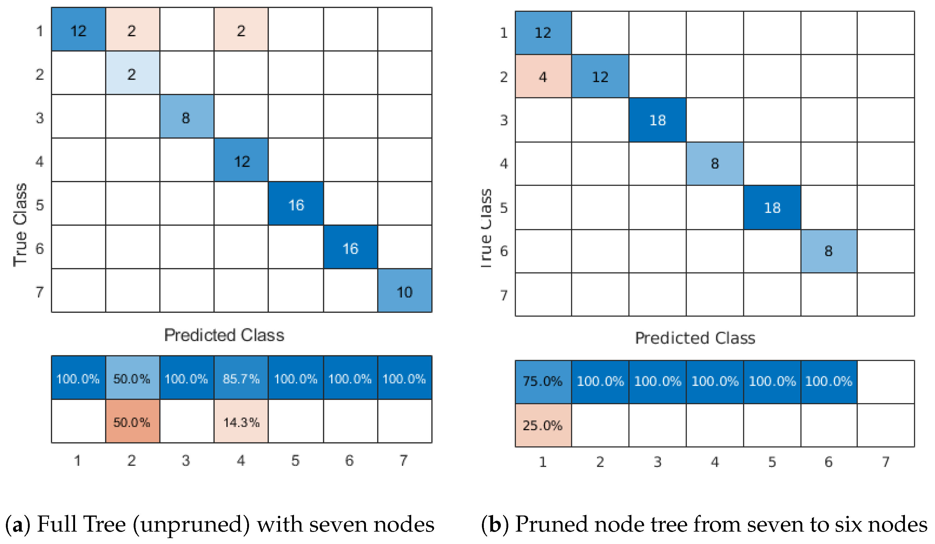
We define as ‘Recognition Accuracy’ the percentage of correctly classified images as containing some corroded area. In the case of our method, this means an image whose predicted dominant cluster contains some arbitrary percentage of captured corroded region above a threshold of
of true positive pixels. For example,
Figure 2 illustrates the case of a confusion matrix for tree nodes
. It is evident that recognition accuracy remains the same at
for pruned and unpruned Eigen tree. Similarly produced confusion matrices for
result in an accuracy of
and
, respectively, (as they appear in
Table 1). As will become evident later, recognition accuracy does not necessarily depend on our pruning method, but rather on the implemented decision criteria as evidenced in
Table 1. We note that there is no direct representation of true coverage versus ground truth in this metric.
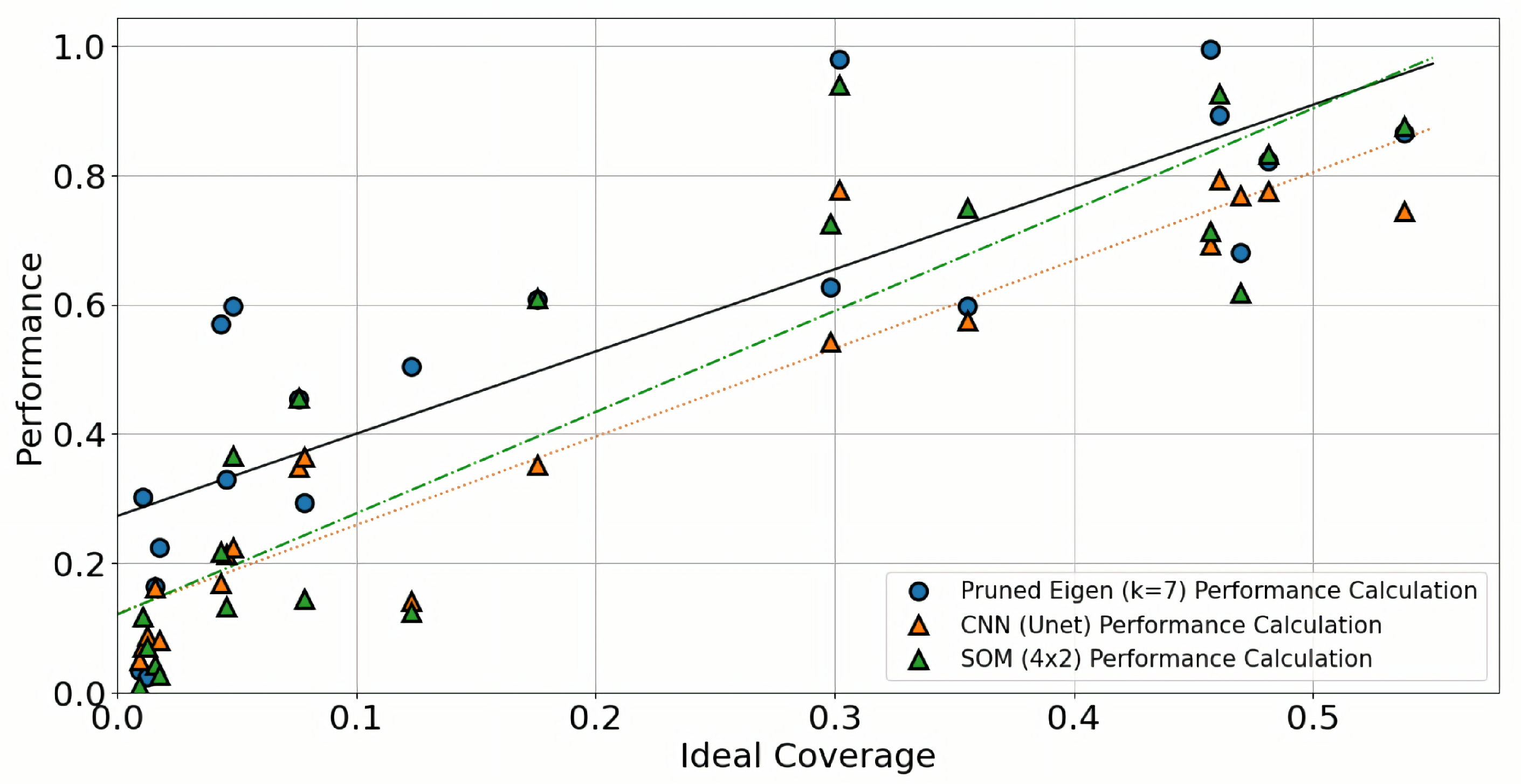
We refer to ‘Ideal Coverage’ as the number of labelled pixels over total image pixels, i.e., percentage of maximum coverage that could be achieved by any given method. This aids the comparison to Ideal Coverage as a reference value. The number of TP pixels over the total number of image pixels is the True ‘Area Coverage’ (TAC), with the number of FP pixels over total number of image pixels being False ‘Area Coverage’ (FAC). The closer TAC is to Ideal Coverage, the higher the expected accuracy in terms of capturing defective pixels. However, FAC can be any given percentage outside of the label region, and as such should be used to ‘penalise’ a method’s performance measure. The ‘Performance’ metric is defined as per the metric:
The metric of Equation (
5) is an indication of the algorithms’ performance, since FAC is not related to ideal coverage and it penalises the method behaviour. The CNN and SOM versus Pruned Eigen tree method comparison is summarised in
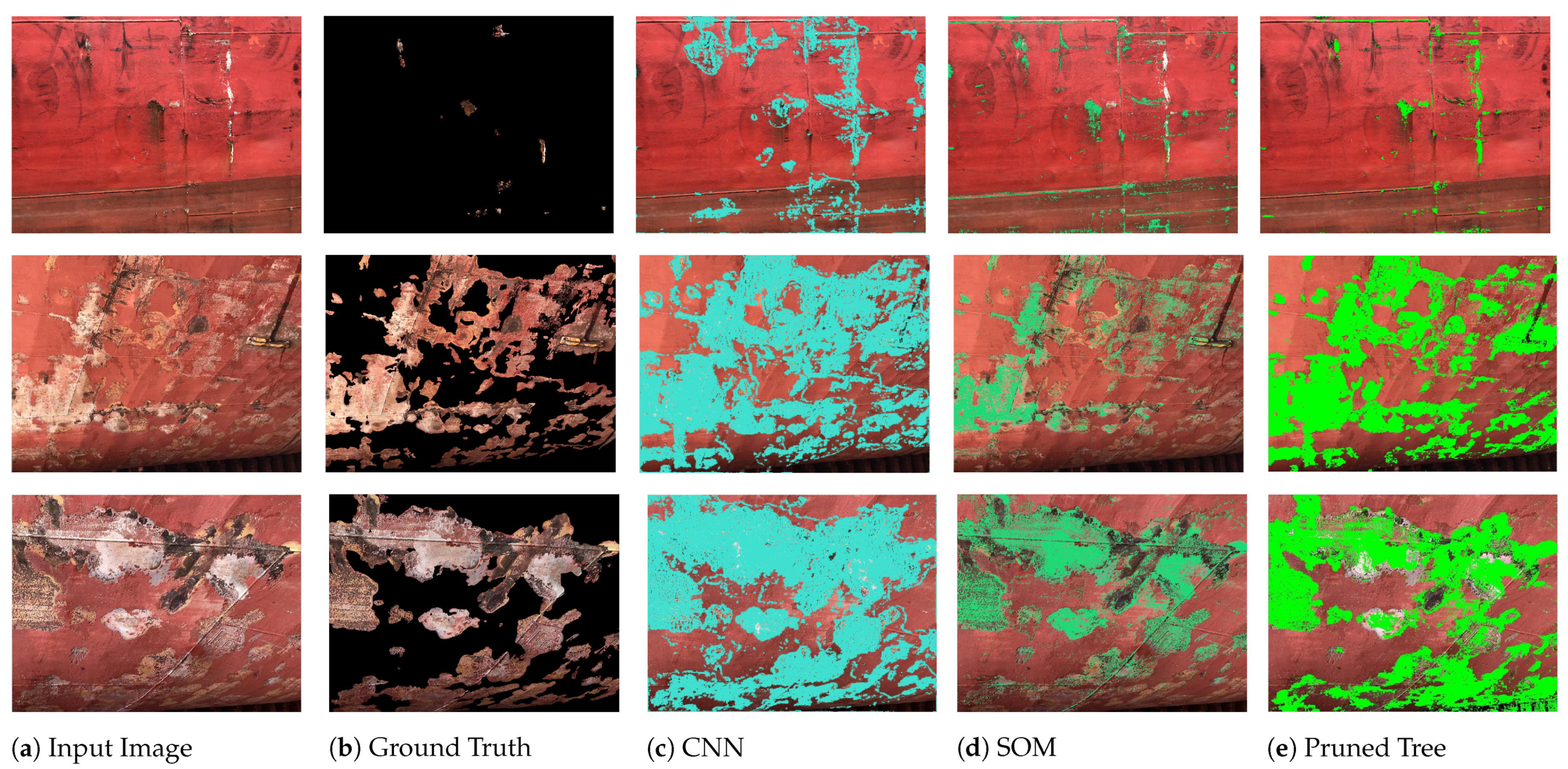
Figure 1, with example results provided visually in
Figure 3.
4. Discussion
We provided evidence that our pruned Eigen tree exhibits better performance than CNN and SOM architectures, by means of
Figure 1 and
Figure 3. We further substantiate this by means of accumulated results in
Table 1, whereas the mean values of the defined metrics over the totality of the dataset instances are reported. It is evident that the implemented CNN architecture (inspired by U-Net) outperforms other techniques under investigation in recognition accuracy. However, and at least for our dataset and annotations, CNN and SOM do not outperform the Eigen tree methods (pruned/unpruned), with respect to Area Coverage ratios and, thus, performance. In fact, on average, the CNN architecture has a better true positive (TP) coverage at the expense of increased false positive (FP) coverage, whilst the remainder of the reported methods seem to be more balanced in the sense of TP/FP area coverage ratios.
Furthermore in
Table 1 the pruned Eigen tree has a significantly higher TP coverage without sacrificing FP coverage, as opposed to the unpruned Eigen tree. The same applies for the CNN and SOM methods, although the number of clusters maximum depth seems to have a minor effect on dominant cluster selection, and thus average performance. Conversely, the pruned Eigen tree has a better TP to FP area coverage, although on aggregate, performances between pruned and unpruned versions of the tree seem to be comparable. For example, in
Table 1 and for our method (Eigen Tree/Pruned Tree) at
, it is evident that the true positive (TP) area detected is higher than the false positive (FP); i.e., 15.8 versus 13.1%, leading to a performance of
. The performance of
is higher than the
achieved in SOM (
ortho-lattice) and CNN methods, since both of these methods have an FP % higher than the TP % (i.e., in SOM the FP to TP area coverage of 16 versus 10%, and for CNN 20 versus 15%).
We note that the applied CNN model has an increased false-positive area coverage (
in
Table 1) which is higher than that of pruned eigen tree (for tree depth of seven nodes, FP area
) and SOM (FP area
). This leads to the inferior (as defined) CNN performance, similar to SOM implementations, but to a much smaller extent. This should not come as a surprise since, as previously mentioned (see
Section 1), neural networks, and similar deep learning techniques, seem to suffer from crack-like pixel groups and changing light conditions, both of which are extensively present in our dataset. For the pruned eigen tree, this can be said to lead to significantly better performance than CNN and SOM, particularly in the case of low ideal coverage. However, it should be noted that SOM seems to outperform CNN and be very close to the pruned Eigen tree in terms of performance at high coverage (
Figure 1).
We recognise that sample size in the used dataset is an issue for CNN training. It remains to be seen whether increasing the data size would lead to better CNN and possibly SOM performance; albeit that the TP to FP ratio examined herein, and the identified CNN, SOM vs. pruned Eigen tree trends, does not seem to support the data size issue. At present, we can postulate that at least for this dataset, the pruned Eigen tree leads to better overall area coverage and performance.
5. Conclusions
We have presented a revised eigen tree decomposition method alongside a pruning methodology/dominant node selection criteria. We have tested and validated these alongside other methods in a domain-specific dataset. The pruning method does not improve recognition accuracy, but substantially increases true positive (TP) area coverage with smaller false positive (FP) areas. The decision criteria, in conjunction with the pruning method, lead to much better FP to TP ratios.
Our method seems to outperform similar unsupervised segmentation (clustering) techniques, which is even more evident in the pruned Eigen tree case. Furthermore, the pruned Eigen Tree method achieves comparable recognition accuracy and better average area coverage in the domain of corrosion detection to neural network architectures; namely the supervised CNN (U-Net-like) model, and the unsupervised SOM model. This is particularly prominent when low ideal coverage images are expected and high TP area coverage is to be desired.
Future work is required to establish whether a data size increase for CNN model training would lead to better performance. We shall further investigate this route by taking a data-driven model and examining the dataset equal distribution of raw and annotated images in predefined low, medium, and high ideal coverage cases.


