Experimental and Numerical Analysis of a Low-Cost Solar Still

Abstract

The ability to treat saltwater to make it suitable for human consumption has long been sought by mankind. More than three-quarters of the earth’s surface is covered with saltwater. Although this water is important for some forms of transportation and fishing, it contains too much salt to sustain human life or agricultural activities. The current work consists of building a low-cost solar still and numerically modeling this device to predict the performance of the solar still without using any experimental measurements. The simulated results were compared with the best experimental values obtained from the water-covering temperatures and desalinated water yield under Brazilian climatic conditions (coordinates: 23°26′31.344″ S and 46°27′27.468″ W). The simulation results were in acceptable agreement with the experimental data. The main results obtained indicate that the solar still has greater efficiency when the volume of water is smaller inside the equipment owing to the lower height of the water and when the global radiation has greater intensity. In addition, numerical modeling allows the analysis of the behavior of the volume fraction over time for water and vapor and indicates better performance in water production after 30 min.

1. Introduction

Demographic growth has grown exponentially since the first Industrial Revolution. The need for more resources to meet the population demand and the inherent growth of industries implies the intensive use of natural resources by the planet. Among natural resources, water is the most precious asset for human life since its consumption is essential for the survival of living beings. More than 70% of the Earth’s surface is covered with water, but most of it is not suitable for direct human consumption. Approximately 97% of the Earth’s water is in the ocean, approximately 2% of the water is stored as ice in the polar region, and only 1% of the total water is available in the form of rivers, lakes, and underground reservoirs for human, plant, and animal needs [1,2].

Currently, approximately 1.2 billion people suffer from water scarcity and intrinsic factors such as food, energy, and health [3]. In addition, the scarcity of treated water directly influences human consumption of brackish water from artesian wells mainly in rural areas, water from streams, reused water, etc. However, the consumption of this type of untreated water directly causes several diseases that are sensitive to human life. It is estimated that approximately 340,000 children are diagnosed with diarrheal diseases worldwide, and 80% of wastewater is discharged into the environment without treatment. It is also reported that approximately 4.5 billion people are at risk of waterborne diseases because of poor sanitation systems [4].

The United Nations (UN) created the Sustainable Development Goals (SDGs) in 2015 with all member states, also known as Global Goals, as a universal call to action to end poverty, protect the planet, and ensure that all people enjoy peace and prosperity by 2030. Among these 17 goals, the UN highlights the sixth goal of ensuring the availability and sustainable management of water and sanitation. This goal envisions attitudes such as achieving universal and equitable access to safe and clean water and expanding international cooperation and capacity-building support for developing countries in water and sanitation-related activities and programs, including water harvesting, desalination, water use efficiency, wastewater treatment, recycling, and reuse technologies [5]. The existence of this goal is crucial because although water is a human right, reality shows that it is still a good that is unattainable for all.

According to the World Water Council [6], water consumption will increase exponentially in the next 30 years, which will result in a more difficult situation in the future because of our current method of consuming and using water, in addition to the pollution of the small fraction available. The increase in demand for water and food would be between 40% and 50% to supply and feed an additional two billion people worldwide. In the emerging BRICS economic development bloc, where Brazil is located, the increase in water consumption is expected to jump from 1900 km³ to up to 3200 km³.

With the ever-decreasing availability of freshwater resources, the desalination of brackish water, river water, or salt water has emerged as a potential strategy to meet current and future demands. Desalination technology using solar energy is used to clean contaminated water and provide drinking water with a lower salt concentration [7]. This process has gained attention compared to other desalination methods (such as multistage flash evaporation, electrodialysis, reverse osmosis, and solvent extraction methods) that require much more energy and are more expensive owing to the required level of technology [8,9,10]. In contrast to other procedures that can be used to obtain potable water, solar distillation is an economical process [11]. This process uses the concepts of condensation and evaporation of water vapor. In addition, this procedure eliminates numerous salts and pollutants found in rivers and seawater [12]. Owing to its relatively low construction and operating costs and durability, this technology is especially popular in remote rural regions [13,14].

Several researchers have developed and improved solar distillers’ performance by changing the equipment design, mostly using integrated technologies. Patel et al. [7] investigated the performance of a modified dual-tilt (tilt angle = 15°) solar distiller mounted with reflectors (UMDSSS) coupled to a partial cooling coil condenser. The researchers used this system to produce potable water from river water during the summer and winter. The maximum output was 11.499 mL/day in summer and 8.212 mL/day in winter, with an average system efficiency of 76.66% and 54.74%, respectively. El-Sebaey et al. [15] fabricated a single-tilt solar desalter using simple materials and developed a three-dimensional multiphase CFD model for equipment that can be used in any geographic location. The results indicate that the simulated and experimental cumulative daily productivities of the single-tilt solar distiller were 1.982 and 1.785 L/m², respectively. Furthermore, the simulated and experimental daily efficiencies for the tested water blade were approximately 16.79% and 15.5%, respectively.

Suresh and Shanmugan [16] used phase change materials (PCMs) such as alumina nanoparticles and fins with a cotton wick (FWCW) to increase the absorption capacity of solar radiation to increase the efficiency of the solar still. In addition, numerical simulations and experiments were performed to provide suitable solutions for the set of materials used. The daily production rate of pure saline water distillate by the solar distiller was increased using a drip-button because of the FWCW absorption capacity of 70.02%, resulting in a daily (24 h) distillate production of 9.429 kg/m² per day, while the effect of water flowing over the glass cover was 13.37%, which was 25% higher than that without PCMs and nanoparticles. Other recent work has attempted to improve simple equipment using different materials, such as the work of Kabeel et al. [17], who used black ink with TiO₂ nanoparticles and increased its efficiency by 6.1%. Jadidoleslami and Farahbod [18] used an absorber plate coated with ZnO nanoparticles and increased their daily production efficiency by up to 16%.

In addition to new materials, other studies have sought to modify the geometry and operation mechanisms of solar stills. Essa et al. [19] built equipment with single tilt and rotating disks integrated into the equipment. The disks are at the rear of the equipment and a part of them is immersed in the water, and they keep rotating all the time and becoming wet to increase the contact surface between the brackish water and solar radiation. The solar water distiller improved by 124% compared with the reference distiller (without the disks). The maximum thermal efficiency was 54.5% for the modified disk solar distillers, working at a speed of 0.05 rpm. From the work exposed above, it is evident that the performance of solar stills depends on factors such as the temperature of the absorber, the temperature of the glass, the material that is absorbing the solar radiation, and the amount of water in contact with the absorber, among others. However, in addition to experimental data, it is important to combine simulations with practice to improve this technology. Therefore, in the present study, a simple solar still developed with low-cost materials is proposed for a comparative analysis between the real thing and CFD numerical simulation. For comparative analysis, studies were conducted with different water volumes (0.5, 1.0, 2.0, and 4.0 L) at different times of the day. In addition, the actual and simulated water production was compared using ANSYS CFD. We believe that this work will contribute considerably to the academic literature, as well as to society, as it can be used as a guide for the construction of this equipment.

2. Materials and Methods

2.1. Development of the Physical Model

The solar still was built following the models available in the literature; however, low-cost materials were used to enable easy replication of the model. Thus, the works of Abderrahmane et al. and Sheva were used as the theoretical basis for the construction of the prototype [20,21]. The main objectives were (1) to develop a low-cost model, (2) to extract the highest efficiency, and (3) to develop a prototype that is minimally resistant to adverse climates (rain and wind). The solar still was built with an inclination angle of 25° towards the south, which is almost the same as the latitude of Guarulhos (Brazil), to ensure that the solar still captures the maximum average radiation during the year. The dimensions of the built model in meters are shown in Figure 1.

The solar still structure was built with medium-density fiberboard (MDF), a wood product manufactured by breaking solid wood into wood fibers and combining them with wax and resin to form panels by applying high temperature and pressure [22]. The advantage of using this material is that it has a value considerably lower than that of conventional types of wood, and with proper protection, it can become considerably water resistant. The main reason for building a prototype using wood composites is that the thermal conductivity of this material is low, which considerably reduces heat loss to the environment and increases the efficiency of the equipment. We used an MDF with a white coating and a thickness of 1.5 cm. The approximate thermal conductivity of MDF is 0.12 W/mK [23]. The white varnish coating on the MDF generates a surface protection film against water so that no penetration into the wood occurs. However, in the project, there will be a quantity of standing water on the surface of the model base, so in addition to this protection, silicone was used on the bottom of the prototype to provide the best isolation against water infiltration into the physical model. The silicone used was from Tekbond and had 100% protection against water infiltration, in addition to being resistant to high temperatures (−30 °C to 150 °C). An aluminum plate was placed at the base of the equipment to promote the optimal use of solar radiation and increase the efficiency of the equipment. Soon, solar radiation penetrates the glass surface and meets the aluminum plate at the base of the equipment, and as aluminum has a high thermal conductivity of 237 W/mK [24], it considerably heats the water in which it is submerged, generating a greater phase change and accelerating the evaporation process. In addition, the equipment was painted black with a high-temperature spray to obtain the best possible absorption of sunlight. The spray used for painting was a Chemi Color matte black model, which is resistant to extreme temperatures of up to 600 °C.

Figure 2 illustrates the process of building a solar-still prototype. Each step can be visualized from the initial modeling of the model using only the structures. The construction process is described as follows.

• Modeled structure with proper dimensions using MDF.
• PVC pipe for the water flow inlet to supply the model with the initial water volume for testing.
• Black silicone was added to the base and corners of the equipment to mitigate the possibility of water leakage in these regions. The PVC gutter for the desalinated water outlet should flow from the glass to the clean water compartment outside the equipment.
• Painting of the entire internal structure to better absorb solar radiation internally.
• Addition of an aluminum plate at the base of the equipment to generate more heating, and consequently, more evaporation. Subsequently, the plate was painted black. In addition, a small aluminum plate can be seen along with the gutter, which prevents clean water from falling out of the gutter.
• Final model of the developed solar still.

2.2. Instrumentation for Obtaining Test Data

The temperature data were obtained with the aid of two thermocouples and a digital thermometer located in three distinct regions of the equipment: the internal part, glass, and aluminum base plate. The thermocouples used were Type K TM-902C with a temperature range of −50 °C to 700 °C and an accuracy of approximately ±0.75%. The thermometer used is generally used in applications where it is submerged in water, has an operating range of −50 °C to 110 °C, and has an accuracy of ±1%. The water electroconductivity data were obtained using a TDS & EC Digital Conductivity Meter (Sigma-Aldrich, Brazil) with an accuracy of ±2% and factory calibration. The global radiation and reflected radiation data were obtained at an automatic meteorological station of Campbell Sci and provided by the Laboratory of Climatology and Biogeography of the Department of Geography of the University of São Paulo (USP), where it is installed, located at coordinates 23°33′47″ W and 46°43′22.98″ S.

2.3. Water Preparation for the Experimental Tests

To create an approximation for seawater, the solutions used were prepared using commercial fluoridated mineral water. The advantage of using water as a solution is that its physicochemical characteristics are available.

Table 1. Physical-chemical characteristics of used mineral water.

pH at 25 °C	Evaporation Residue at 180 °C	Conductivity at 25 °C
7.32	137.51 mg/L	190.6 μS/cm

shows the physicochemical characteristics and

Table 2. Mineral chemical composition of the water used.

Component	Quantity (mg/L)
Barium	0.14
Bicarbonate	100.53
Calcium	4.17
Chloride	0.90
Strontium	0.04
Fluoride	0.94
Magnesium	0.99
Phosphate	0.76
Potassium	2.48
Sodium	32.50
Sulfate	1.75

shows the chemical composition values in mg/L.

The chemical composition of dissolved salts in seawater has been estimated with some precision in the literature because the salinity of the ocean has been stable for millions of years. Thus, a widely used value to represent the mass of dissolved salts in seawater is 3.5% of the total volume, with a range between 3.3% and 3.7% [25,26], and these deviations occur at the surface owing to processes such as evaporation and precipitation [27]. The presence of dissolved salts in water consequently creates electrical conductivity in the medium owing to the movement of electrically charged particles in response to the forces acting on them from an applied electric field. In water, salts, such as sodium chloride (NaCl), disassociate to form cations (Na⁺) and anions (Cl⁻) that migrate in the presence of an electric field, thus producing an electric current. The conductivity σ increases with the concentration of dissolved salts and with increasing temperature T, which can be reasonably associated with an increase in ion mobility [28]. The electrical conductivity of seawater is in the range of 46,000–72,000 μS/cm [29].

Thus, knowing the mass concentration values and electrical conductivity of the sea from the literature, it is possible to prepare a solution with similar properties. In this study, commercial refined sea salt was used to supplement the number of salts dissolved in the mineral water until the electrical conductivity values were similar to those of ocean water.

Table 3. Nutritional information of salt (a portion of 1 g).

Component	Mass (mg)
Sodium	390
Iodine	0.025

lists the nutritional information of the salts used in this study.

Four solutions with different volumes were prepared for the experimental tests. The amount of commercial salt was placed respecting the value of approximately 3.5% of the total volume. The electrical conductivity of water was measured using a conductivity meter.

Table 4. Characteristics of the solutions for the experimental test.

Sample	Volume (L)	Mass of Salt (g)	Conductivity (μS/cm)
1	0.5	17.5	61,050
2	1.0	35	64,520
3	2.0	70	61,760
4	4.0	140	54,580

shows the volume of the four samples and their final electrical conductivities. The conductivity values were close to the theoretical range for seawater.

2.4. Energy Balance of the Solar Still Behavior

Three energy balances were performed to describe the behavior of the solar still, i.e., energy balance for the water mass in the equipment, energy balance for the glass cover, and energy balance for the basin liner. Studies by Abu-Khader et al., Akram et al., and El-Sebaey et al. [15,30,31] were also considered. This balance is discussed below.

The basin water–energy balance equation can be written as

$$I_1+Q_b+C_{H_{2}O}=\frac{d{T}_{H_{2}O}}{dt}+Q_{c{H}_{2}O}+Q_{r{H}_{2}O}+Q_{e{H}_{2}O}+I_2$$

(1)

where Q_b is the heat transfer by convection from the basin to the water, C_H2O is the specific heat of the water in the basin, T_H2O is the temperature of the water in the basin, Q_eH2O is the heat transfer by evaporation from the water to the glass, Q_rH2O is the heat transfer by radiation from the water to the glass, Q_cH2O is the heat transfer by convection from the water to the glass, I₁ is the solar intensity falling on the surface of the water after transmission through the glass, and I₂ the solar intensity falling on the basin liner after passing through the water mass. I₁ and I₂ can be expressed as

$$I_1=\left(1-{\alpha }_v\right)I$$

(2)

$$I_2=\left(1-{\alpha }_v\right)\left(1-{\alpha }_{H_{2}O}\right)I$$

(3)

where α_v is the radiation absorptivity of the glass, is the radiation absorptivity of the water, and I is the available solar intensity at the site in W/m². Radiation heat transfer occurs between the water surface and glass cover owing to the temperature difference, according to the Stefan-Boltzmann law:

$$Q_{r{H}_{2}O}=h_{r{H}_{2}O}{A}_{H_{2}O}\left(T_{H_{2}O}-T_v\right)={\epsilon }_{eff}{A}_{H_{2}O}\sigma \left(T_{H_{2}O}{}^4-T_v{}^4\right)$$

(4)

$$h_{r{H}_{2}O}={\epsilon }_{eff}\sigma \left(\left(T_{H_{2}O}{}^2-T_v{}^2\right)\left(T_{H_{2}O}{}^2-T_v{}^2\right)\right)$$

(5)

where h_rH2O is the radiated heat transfer coefficient between the water and glass, A_H2O is the water cross-sectional area of the basin, σ is the Stefan–Boltzmann constant (5.67 × 10⁻⁸ W/m²K⁴), and ε_eff is the Effective Emittance between the water surface and glass cover.

The heat transfer rate from the water surface to the glass (Q_cH2O) by convection through moist air in the upward direction is given by

$$Q_{c{H}_{2}O}=h_{c{H}_{2}O}{A}_{H_{2}O}\left(T_{H_{2}O}-T_v\right)$$

(6)

The rate of heat loss owing to evaporation (Q_eH2O) can be determined using the following expression:

$$Q_{e{H}_{2}O}=h_{e{H}_{2}O}{A}_{H_{2}O}\left(T_{H_{2}O}-T_v\right)$$

(7)

where h_cH2O and h_eH2O are the convective heat transfer coefficients and evaporative heat transfer coefficients, respectively. The energy balance equation in glass can be defined as

$$Q_{rv}+Q_{cv}+I_1=I+Q_{e{H}_{2}O}+Q_{r{H}_{2}O}+Q_{c{H}_{2}O}$$

(8)

where Q_cglass is the convective heat transfer from glass to the atmosphere, I is the solar radiation falling on the solar still, and Q_rglass is the radiated heat transfer from glass to the atmosphere. Q_rglass can be expressed as

$$Q_{rglass}={\epsilon }_{glass}{A}_{glass}\sigma \left(T_{glass}{}^4-T_{sky}{}^4\right)=h_{rglass}{A}_{glass}\left(T_{glass}-T_a\right)$$

(9)

where A_glass is the surface area of the glass exposed to the atmosphere, h_rglass is the coefficient of heat transfer by radiation between the glass and atmosphere, T_a is the atmospheric temperature, and T_sky is the sky temperature that is lower than (such as 6 °C) the ambient temperature. The convective heat transfer from the glass to the atmosphere is

$$Q_{cglass}=h_{cglass}{A}_{glass}\left(T_{glass}-T_a\right)$$

(10)

where h_cglass is the convective heat transfer coefficient between the glass and the atmosphere. The heat balance equation in the basin lining can be written as

$$I=Q_b+Q_{ba}$$

(11)

$$Q_{ba}=U_{ba}{A}_b\left(T_b-T_a\right)$$

(12)

where Q_ba is the heat transfer rate from the basin liner to the atmosphere through the bottom side and U_ba is the overall heat transfer coefficient between the water basin liner and the atmosphere. The convective heat transfer from the basin liner to the water can be expressed as

$$Q_b=h_b{A}_b\left(T_b-T_{H_{2}O}\right)$$

(13)

where h_b is the convective heat transfer coefficient between the basin liner and the water.

2.5. Numerical Simulation Using Computational Fluid Dynamics (CFD)

In this study, ANSYS Fluent 2020R2 (Pennsylvania, United States) was used to solve the governing equations of the problem. Fluent is an extremely robust software capable of solving cases from aerothermodynamics to reactive and multiphase flows and is a reference in industry and academia for its potential.

2.6. Geometry Development and Mesh Generation

The geometry developed for the virtual prototyping of the solar still was built using the ANSYS SpaceClaim Software, which is a tool for modeling and repairing 3D solids. The developed model follows the dimensions of the physical prototype; however, it has a rectangular trough zone created in a simpler manner than the real model to capture desalinated water. A simplification was generated to minimize the excessive number of mesh elements and to facilitate the convergence of the numerical model. Figure 3 shows the geometry created.

The meshing process was performed using ANSYS Meshing Tools software. Initially, a fully hexahedral mesh was generated owing to its fast convergence and easy adaptation in considerably simple geometries; however, in the present case, the inclination of the glass generated distorted elements near the gutter when it came to a mesh essentially represented by hexahedral elements. Thus, the model was divided into three parts: the lower part that will have standing water and the solar still body was initially represented by hexahedral elements, and the rest of the geometry was represented by tetrahedral elements to better capture the effects of the model with a smaller mesh resource, given that the tetrahedral mesh has an easier time working with more complex and non-rectilinear geometries. To create a transition between the elements, the Share topology feature was used to connect the different bodies of the geometry, which is crucial for generating a conformal mesh, preserving the connection of the nodes between the elements.

To evaluate the mesh quality, the “Orthogonal Quality” method was used, which is calculated by considering the vector normal to each face of the tetrahedron. The cosines between faces were calculated by defining the orthogonality of the mesh. It considers the vectors normal (A_i) to the element face, vectors between the centroids of the cell and midpoint of the faces (f_i), vectors between adjacent cell centroids (C_i), and vectors between the centroids of the face and medians (e_i).

Using this method, a mesh is considered to be of good quality when its quality value is close to 1. The average mesh quality of the solar still computational domain was 0.89, which was classified as very good quality [32]. A mesh independence study was performed to analyze the mesh density and error associated with the discretization process. Three grids of different densities (coarse, medium, and fine) were generated, and the amounts of water produced were compared.

Table 5. Grid independence test.

Grid	Number of Cells	Produced Water (L)	Error (%)
1	643,648	0.062	-
2	1,449,227	0.071	15%
3	2,268,312	0.072	1%

presents the results and error associated with each mesh. Therefore, with a small difference between the fine and medium grids, grid independence was achieved, and grid 2 could be used for the numerical simulation. Figure 4 shows the generated mesh.

2.7. Turbulence Model

Turbulence flows are characterized by the chaotic motion of fluid particles. It is generally characterized by irregularity, diffusivity, large Reynolds numbers, three-dimensional vorticity fluctuations, and dissipation. Unsteady, irregular (aperiodic) motion in which transported quantities (mass, momentum, and scalar species) fluctuate in time and space. Turbulence models are required to solve the unknown variables. The correct analysis of problems involving turbulence is the biggest challenge in CFD modeling. Therefore, for the type of application of the present work, although the flow velocity is commonly low, the natural convection in the vapor has the characteristics of a turbulent flow, which implies the need for a turbulence model to be able to capture the physical effects correctly, as studied by Rahman et al. [33] in the Rayleigh number analysis in a similar study. The main turbulence models are as follows:

• Direct Numerical Simulation (DNS);
• Large Eddy Simulation (LES);
• Reynolds Averaged Navier Stokes Simulation (RANS).

DNS consists of a direct numerical model capable of solving turbulent flow with all its phenomena and all scales of turbulence, with results very close to those of physical experiments. However, the use of this model requires an extremely robust computational resource, as its solution requires an extremely refined mesh to capture the effects of small scales of turbulence; therefore, the use of this model is not feasible in everyday engineering. A direct alternative to this model is the use of large-scale turbulent simulations (LESs). In this type of simulation, coarser meshes than DNS meshes are used, but they are fine enough to capture turbulent structures down to the inertial scale. However, the computational cost of large-scale simulations is also quite high, making this technique a useful tool, but also unattractive for day-to-day industrial applications [34]. On the other hand, the Reynolds Average Approach (RANS) model generally consists of turbulence modeling rather than turbulence resolution, that is, this model is an approximation for reproducing the average behavior of turbulence effects in the flow. RANS models have several specific characteristics, but one of the most widely used is the two-equation RANS model based on the Boussinesq hypothesis. The models used mathematical relationships to insert the effect of turbulence into the average behavior of the flow with the aid of the Reynolds time average. The main benefit of this methodology is that the computational cost of these models is much lower than that of models that solve for turbulent scales [35]. Thus, the RANS model is the most widely used in everyday engineering.

The standard k–ε models in ANSYS Fluent fall into the class of RANS models and have become the most widely used because they were proposed by Launder and Spalding [35]. There are three versions of this model in Fluent: the standard, RNG, and realizable k–ε models. All three forms are similar to the transport equations for k and ε. The standard k–ε model is based on the transport equations for turbulence kinetic energy (k) and its dissipation rate (ε). The k transport model equation was derived from the exact equation, whereas the transport model equation for ε was obtained using physical reasoning. The RNG k–ε model was developed to overcome some of the limitations of the standard model. The RNG model was derived using a statistical technique called renormalization group theory [36,37,38]. It is similar in form to the standard k-ε model but includes the following refinements [39]:

• The RNG model has an additional term in its equation (ε), which improves the accuracy of rapidly deformed flows.
• The effect of swirl on turbulence was included in the RNG model, increasing the accuracy of the swirling flows.
• The RNG theory provides an analytical formula for turbulent Prandtl numbers, whereas the standard k model uses user-specified constant values.
• While the standard model is a high Reynolds number model, the RNG theory provides an analytically derived differential formula for the effective viscosity that takes into account the low Reynolds number effects. However, the effective use of this feature depends on the proper treatment of the near-wall region.

These features make the k–ε RNG model more accurate and reliable for a broader class of flows than the standard k–ε model. Furthermore, the choice of the k-ε RNG model is based on similar studies that use this model and acquire good results compared to the experimental test, for example, the studies of El-Sebaey et al. and Keshtkar et al. [15,40].

Thus, this was the model used in this work, and its mathematical formulation for a transient case can be expressed in Equations (14) and (15) [37,41]:

$$\frac{\partial }{\partial t}\left(\rho k\right)+\frac{\partial }{\partial x_i}\left(\rho k{u}_i\right)=\frac{\partial }{\partial x_j}\left({\alpha }_k{\mu }_{eff}\frac{\partial k}{\partial x_j}\right)+G_k+G_b-\rho \epsilon -Y_M+S_k$$

(14)

$$\frac{\partial }{\partial t}\left(\rho \epsilon \right)+\frac{\partial }{\partial x_i}\left(\rho \epsilon u_i\right)=\frac{\partial }{\partial x_j}\left({\alpha }_{\epsilon }{\mu }_{eff}\frac{\partial \epsilon }{\partial x_j}\right)+C_{1\epsilon \frac{\epsilon }{k}}\left(G_k+C_{3\epsilon }{G}_b\right)-C_{2\epsilon \rho \frac{{\epsilon }^2}{k}}-R_{\epsilon }+S_{\epsilon }$$

(15)

In these equations, G_k represents the kinetic energy generation of turbulence owing to mean velocity gradients. G_b is the turbulence kinetic energy generated owing to buoyancy. Y_M represents the contribution of the buoyant dilatation in compressible turbulence to the overall dissipation rate. The quantities α_k and α_ε are the effective inverse Prandtl numbers of k and ε, respectively. S_k and S_ε are user-defined source terms. C_1ε and C_2ε are constants defined as 1.42 and 1.68, respectively. The term R_ε is defined as

$$R_{\epsilon }=\frac{C_{\mu }\rho {\eta }^3\left(1-\frac{\eta }{{\eta }_0}\right)}{1+\beta {\eta }^3}\frac{{\epsilon }^2}{k}$$

(16)

where η = S_k/ε, η₀ = 4.38, and β = 0.012.

2.8. Multiphase Model

Multiphase flows are flows in which more than one phase of matter is present, with liquid, gas, and solid phases. In general, the applications of these flows consist of flows where there is a liquid or gas phase, for example, an evaporating liquid where there is a liquid phase and vapor (gas phase). In a multiphase flow, a phase can be defined as an identifiable class of material that has a particular inertial response and interaction with the flow and potential field in which it is immersed.

Advances in computational Fluid Dynamics have provided a basis for further insights into the dynamics of multiphase flows. Currently, there are two approaches to the numerical calculation of multiphase flows:

• Euler–Lagrange;
• Euler–Euler.

In the Euler–Lagrange approach, the fluid phase is treated as continuous by solving the Navier–Stokes equations, whereas the dispersed phase is solved by tracing a large number of particles, bubbles, or droplets through the calculated flow field. The dispersed phase exchanges momentum, mass, and energy with the fluid phase. In the Euler–Euler approach, on the other hand, the different phases are treated mathematically as interpenetrating continua. Because the volume of one phase cannot be occupied by the other phases, the concept of phase volume fraction is introduced. These volume fractions are considered continuous functions of space and time, and their sum is equal to one. The conservation equations for each phase were derived to obtain a set of equations that have a similar structure for all phases. These equations are closed by providing constitutive relations that are obtained from empirical information or, in the case of granular flows, by applying the kinetic theory.

The Volume of Fluid (VOF) model is a Euler–Euler approach in which a single set of momentum equations is shared by the fluids, and the volume fraction of each of the fluids in each computational cell is tracked across the domain. This model was used in the present work because it is computationally lighter and provides good results when coupled with mass transfer models. In addition, the VOF model was used in a similar recent study and showed good results [15].

In the solution procedure, the governing equations for the conservation of mass, momentum, and energy are described in the next Equations (17)–(19).

$$\frac{\partial \rho }{\partial t}+\nabla ·(\rho \overrightarrow{v})=0$$

(17)

A single momentum Equation (18) was solved over the entire domain, and the resulting velocity field was shared between the phases. The momentum equation shown below is dependent on the volume fractions of all phases via the properties of density (ρ) and viscosity (μ).

$$\frac{\partial }{\partial t}(\rho \overrightarrow{v})+\nabla ·(\rho \overrightarrow{v}\overrightarrow{v})=-\nabla \rho +\nabla ·[\mu (\nabla \overrightarrow{v}+\nabla {\overrightarrow{v}}^T)]+\rho \overrightarrow{g}+\overrightarrow{F}$$

(18)

where $\overrightarrow{F}$ is the resultant body force of the surface tension at the interface.

$$\frac{\partial }{\partial t}\left(\rho E\right)+\nabla ·(\overrightarrow{v}\left(\rho E+p\right))=\nabla ·(k_{eff}\nabla T-{{\displaystyle \sum }}_q{{\displaystyle \sum }}_j{h}_{j,q}{\overrightarrow{j}}_{j,q}+({\overline{\tau }}_{eff}·\overrightarrow{v}))+S_h$$

(19)

where k_eff is the effective conductivity k + k_t, where k_t is the turbulent thermal conductivity defined according to the turbulence model used), ${\overrightarrow{j}}_j$ is the diffusion flux of species j, h_j,q is the enthalpy of species j in phase q, and ${\overrightarrow{j}}_{j,q}$ is the diffusive flux of species j in phase q. The first three terms on the right-hand side represent energy transfer due to conduction, species diffusion, and viscous dissipation, respectively. S_h includes the volumetric heat sources.

The interface(s) between the phases is tracked by solving a continuity equation for the volume fraction of one (or more) of the phases. For the qth phase, this equation has the following form:

$$\frac{1}{{\rho }_q}\left[\frac{\partial }{\partial t}\left({\alpha }_q{\rho }_q\right)+\nabla ·({\alpha }_q{\rho }_q{\overrightarrow{v}}_q)=S_{\alpha q}+{{\displaystyle \sum }}_{p=1}^n\left({\dot{m}}_{pq}-{\dot{m}}_{qp}\right)\right]$$

(20)

where ${\dot{m}}_{qp}$ is the mass transfer from phase q to phase p; ${\dot{m}}_{pq}$ is the mass transfer from phase p to phase q; α is the volume fraction; and ρ is the phase density. By default, the source term $S_{\propto q}$ on the right-hand side is zero; however, a constant or defined mass source can be specified for each phase. The phase-change flow rate $\dot{m}$ can be caused by evaporation or condensation at the interface, positive or negative, respectively. Lee’s phase change model was applied to consider this mass transfer. In Lee’s model [42,43], the liquid–vapor mass transfer (evaporation and condensation) is governed by the vapor transport Equation (21).

$$\frac{\partial }{\partial t}\left({\alpha }_v{\rho }_v\right)+\nabla ·\left({\alpha }_v{\rho }_v{\overrightarrow{V}}_v\right)={\dot{m}}_{lv}-{\dot{m}}_{vl}$$

(21)

where v is the vapor phase, α_v is the vapor volume fraction, ρ_v is the vapor density, ${\overrightarrow{V}}_v$ is the vapor phase velocity, ${\dot{m}}_{lv}$ and ${\dot{m}}_{vl}$ are the mass transfer rates due to evaporation and condensation, respectively, which can be defined according to Equations (22) and (23).

If T₁ > T_sat (Evaporation):

$${\dot{m}}_{lv}=coeff{\alpha }_l{\rho }_l\frac{\left(T_l-T_{sat}\right)}{T_{sat}}$$

(22)

If T₁ < T_sat (Condensation):

$${\dot{m}}_{vl}=coeff{\alpha }_v{\rho }_v\frac{\left(T_{sat}-T_v\right)}{T_{sat}}$$

(23)

C_oeff is a coefficient that must be adjusted and can be interpreted as the relaxation time, α is the phase volume fraction, and ρ is the density.

2.9. Boundary Conditions

Owing to the complexity of the simulation, computational resources, and simplification, when building the CFD simulation model, some assumptions have to be considered, as follows:

• There is no thermal source inside the solar still.
• The effect of the wind speed was neglected, and only free convection was considered.
• No leakage occurred in this system. In addition, the bottom and side walls of the distiller were maintained at a constant temperature.
• The water level inside the basin was kept constant.
• Because the temperature variation was low, fluid properties such as density, thermal conductivity, specific heat, and viscosity were considered as piecewise linear profiles with temperature, while the physical properties of the walls were considered constant.
• Evaporation and condensation occur mainly by temperature and not pressure. The saturation temperature was set as a constant, with the first water production value of 53 °C as a reference.

The boundary conditions for the model were extracted based on the average data extracted from Test 3, where the water level inside the physical equipment was initially 2 L of water. Thus, with the values of the boundary conditions imposed at the end of the calculation, the clean water production can be validated with the values obtained in the experimental study.

Table 6. Input parameters used in the CFD simulation.

Function	Configuration
Solver	Geometry	3D
	Time	Transient
	Turbulence	Model RNG k-epsilon
	Multiphase	Model Volume of Fluid (VOF)
Materials	Solid	Glass
		Aluminum
		Wood
	Fluid	Air
		Vapor water
		Liquid water
Phases	Primary Phase	Air
	Secondary Phase	Vapor water
		Liquid water

lists the input parameters and

Table 7. Boundary conditions used in the CFD simulation.

Region	Type	Thermal Conditions	Temperature (°C)
Glass	Wall	Constant Temperature	43
Base	Wall	Constant Temperature	70
Wall	Wall	Constant Temperature	59
Gutter	Wall	Constant Temperature	27

lists the boundary conditions for the CFD model.

The solution parameters used, that is, the methods selected for the pressure–velocity coupling, are listed in

Table 8. Solution parameters used in CFD simulation.

Function	Configuration
Solutions Methods	Pressure-velocity Coupling	SIMPLE
	Spatial Discretization	Gradient	Least Squares Cell-Based
		Pressure	PRESTO
		Moment	Second order Upwind
		Density	Second order Upwind
		Volume Fraction	Compressive
		Energy	Second order Upwind

. To achieve convergence, the residuals were monitored for the X, Y, and Z velocities, continuity, energy, turbulent kinetic energy (k), and the kinetic energy dissipation rate (ε). The convergence criterion for the energy equation was 10⁻⁶. The convergence criterion for all other variables was taken as 10⁻³.

3. Results

3.1. Experimental Results

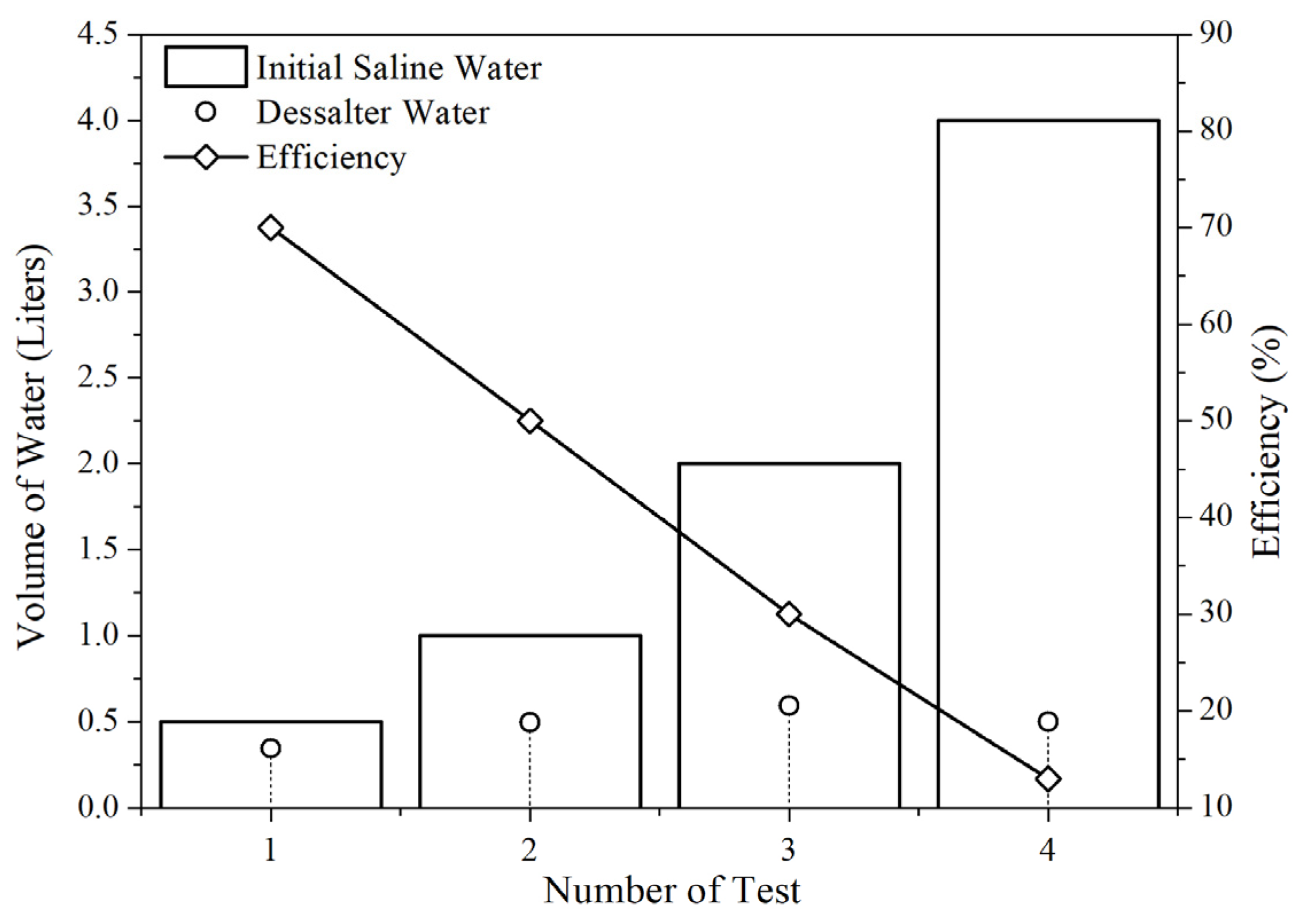
The experimental tests were performed over four days with different initial water volumes in the equipment, being 0.5 L, 1 L, 2 L, and 4 L. The tests were performed from 9:00 am to 17:00, as this is the time when the model receives the most solar radiation and consequently has its peak efficiency. The tests were performed in the city of Guarulhos-SP under the coordinates 23°26′31.344″ S and 46°27′27.468″ W with the equipment oriented north to receive the greatest solar radiation. The results show that for a volume of 0.5 L, the production of desalinated water was 0.345 L, for 1 L, the production was 0.495 L, for 2 L, the production was 0.593 L, and for 4 L, the production was 0.500 L. By directly analyzing the mentioned values, it was possible to ascertain that the direct efficiency considering the initial water volume and that produced in the equipment was approximately 69% for the first test, 50.5% for the second, 29.65% for the third, and 12.5% for the fourth.

Figure 5 shows the results obtained for the desalinated water production and efficiency. It can be seen that the highest efficiency in the model occurs in the first test, where there is a low volume of water in the prototype, and then the efficiency decreases as the volume increases in the later tests. Physically, it is possible to understand this effect as a consequence of the increase in the height of the water inside the prototype, because with this increase, there is more volume and, consequently, more energy is needed to heat the fluid and start the evaporation process. This effect was also observed by Rajaseenivasan et al., who observed a 20% decrease in water volume with increasing blade height [44]. Naturally, the decrease in water volume is also due to other factors, such as the radiation incident on the model, which is a determinant to understand. For example, the decrease in the volume of water produced in test four about test three, because despite an ascending production until the third test, there is a drop in production in the fourth.

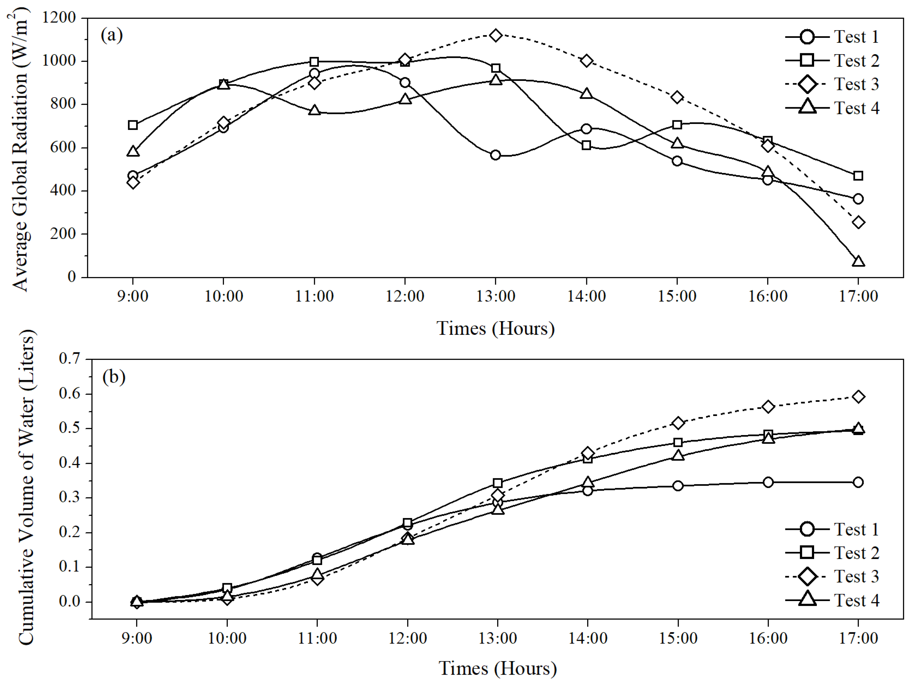
Figure 6a shows the average global radiation for each experiment and the operating hours. The average global radiation was calculated considering the average global radiation for each hour. It can be observed that Test 3 presented the best radiation index among the other tests, and it is possible to observe that the radiation behavior characteristically has a knee-shaped curve with higher radiation in the period from 11:00 to 14:00, indicating consistent meteorological behavior without many variations in the day. Observing the behavior of radiation in Test 3 in comparison with Test 4, the previous analysis of the relationship of clean water production higher in the third test due to radiation is corroborated, given that the values for this day are more consistent than those for the fourth day. The first test presented low radiation on the day; however, the considerable efficiency value may be due to the smaller water volume (smaller water blade), as observed previously. Regarding Test 2, the radiation presents a drop at approximately 14:00, but still, the production for this day can be considered good when related to the other days. Figure 6b shows the water production with the cumulative volume for all the tests. It can be seen that the behavior of the tests is similar during the day; exceptionally, Test 3 shows a higher water production. However, this is due to the positive weather conditions on the day of the test. In addition, the water production in Tests 2 and 4 is very close, which may be related specifically to the low radiation potential on the day of the fourth test. Another possible analysis to be performed refers to the production limit of the equipment because the values were stagnant at approximately 0.5 L; however, this statement would require more physical tests and variations of the model geometry to be corroborated.

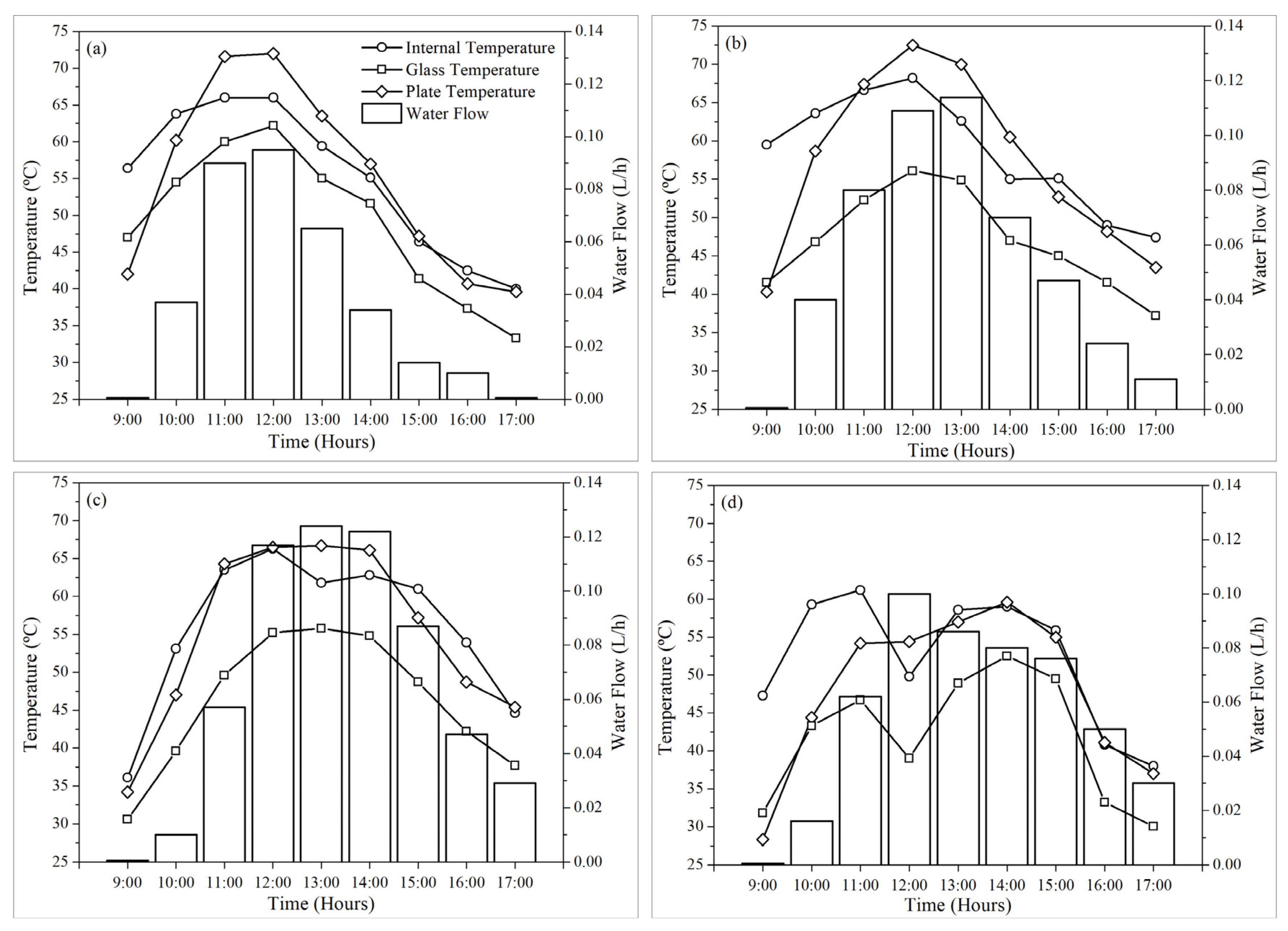
Figure 7a–d demonstrates the behavior of the desalinated water flow rate and the behavior of the internal temperature, glass, and plate for the tests performed. In these figures, it is interesting to analyze the effect of temperature on desalinated water production. Naturally, when temperatures are higher, especially the plate and internal temperatures, water production tends to be higher because the entropy of the process is increased, and, therefore, more evaporation occurs in the system. For condensation to occur, the glass temperature must always be below the plate temperature. Figure 7a shows the behavior of the temperature for the first test with water (0.5 L). The time with the highest water production occurred from 11:00 to 13:00. Although the global radiation was not the highest for this test, because the volume of water was small and, therefore, the height of the slide was also small, the temperature of the aluminum plate reached values higher than 70 °C. Therefore, a larger gradient of water was produced in this test. Figure 7b illustrates the behavior of the temperature and flow rate in Test 2. On the day of this test, water production was better utilized again from 11:00 to 13:00. An observation that can be made from these results is that the internal temperature in the solar still shows good insulation of the wood from the external environment, because even during periods in which the temperature of the plate and glass decreases more rapidly, the internal temperature is maintained for a longer period, demonstrating the usefulness of wood for having low conductivity. Figure 7c illustrates the behavior of the temperature and flow rate for Test 3. On the day of the third test, the period of the highest water production was from 12:00 to 14:00. It is interesting to analyze the affinity of the plate temperature with the global radiation for the same day in Figure 7b because the behavior is directly proportional between the variables because solar radiation is the only source of energy for the system. Another analysis that can be performed on this day is that despite having higher radiation, the model presents a plate temperature lower than the previous models; however, this fact can be justified by the larger volume of water and higher height of the water blade to be heated. Figure 7d illustrates the behavior of the temperature and flow rate for Test 4. The hours of highest water production for this day were from 12:00 to 14:00. From the results shown in Figure 7b,d, it is evident that owing to the variable meteorological conditions on this day, the results were impaired, inferring a low-temperature condition in the model. The 4 L of water volume used in this test is also a factor that makes the overall heating of the water and the desalination process slightly more difficult. Figure 7d also shows that in the 12 h period, although the internal and glass temperatures decreased considerably, the water production was the highest for the test, which can be explained by the constancy in the temperature of the plate during the previous time and the higher condensation owing to the low temperature of the glass.

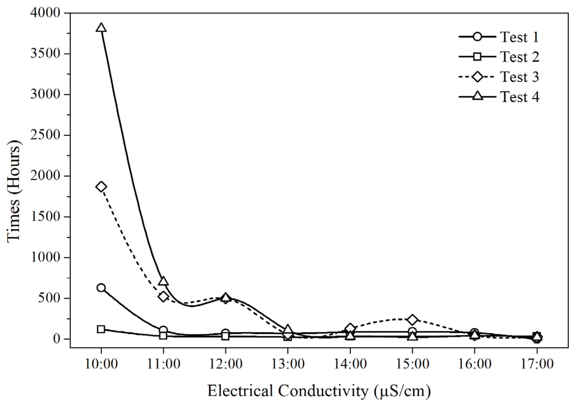
A good parameter for analyzing the effectiveness of the solar desal-water desalination process is based on analyzing the number of dissolved salts in the water after it leaves the equipment. The electrical conductivity (EC) measures the ionic process of a solution that allows the transmission of an electric current. Therefore, the higher the electrical conductivity of water, the greater the number of salts dissolved in the solution [45]. This parameter does not identify the ions present in the water, but it is an important indicator of possible pollutant sources. Figure 8 shows the results obtained for the electrical conductivity of the water that exited the desalter. The results always indicate a higher electrical conductivity of the first water collected from the tests, and this factor is justified by the fact that the first water carries particles stopped in the equipment and can be considered as an initial experimental error. However, analyzing the value of the electrical conductivity of the water placed in the equipment in Table 4, the first results demonstrate the effectiveness of the equipment. However, according to the World Health Organization (WHO) standards, electrical conductivity should not exceed 400 μS/cm [46,47]. Thus, by analyzing Figure 8, it is possible to verify that the results obtained for all tests demonstrate excellent quality because most data are below 400 μS/cm and only a few values are slightly above, in the range of 500–700 μS/cm.

3.2. Numerical Simulation (CFD)

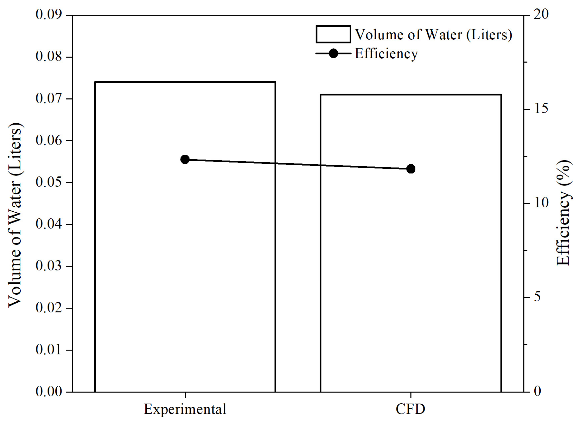
The numerical simulation of the heat and mass transfer was performed using ANSYS 2020R2 software. The simulation was performed for one hour with an initial temperature of 59 °C inside the solar still and an initial water volume of 2 L, similar to Test 3. The results showed that the water production by condensation was 0.071 L, which is a physically consistent value considering that the third test produced an average of 0.074 L of water. Naturally, the values between the prototype and the physical model must have a discrepancy owing to the considerations and simplifications made in the numerical model. It is important to note that the boundary conditions used for the numerical model are based on the tests, so it is possible to perform a validation of the numerical model when considering Test 3 because the temperatures and water volume of 2 L are common to both. Figure 9 shows the values obtained from the numerical simulation and experimental Test 3. A variation of approximately 4% is observed between the two models. Considering the simplifications made in the numerical model, this case can be considered validated owing to the affinity of the values.

Solar still efficiency is the ability of equipment to desalinate saltwater [15]. The ratio between the total amount of thermal energy used to produce water productivity in a given period and the energy supplied to the equipment during the same period is defined as the efficiency of the solar thermal still. Figure 9 shows the efficiency of water production compared to the results for the most critical period analyzed using the simulation in Test 3. The results show an efficiency of 12.3% for the experimental test and 11.8% for the simulation comparing the 1h production of this period with the total water produced in the day. The simulation efficiency was slightly lower than the simulated amount, indicating an acceptable agreement between the simulated and experimental values.

Figure 10 shows the temperature distribution on an intermediate plane along the Z-axis of the numerical model. It can be seen that there is a slight variation in the overall temperature gradient and in the gutter region owing to the volume of water that accumulates over time. As expected, the temperature gradient was higher in the aluminum plate for the evaporation process to occur and lower in the gutter, so that the condensed water remained in liquid form.

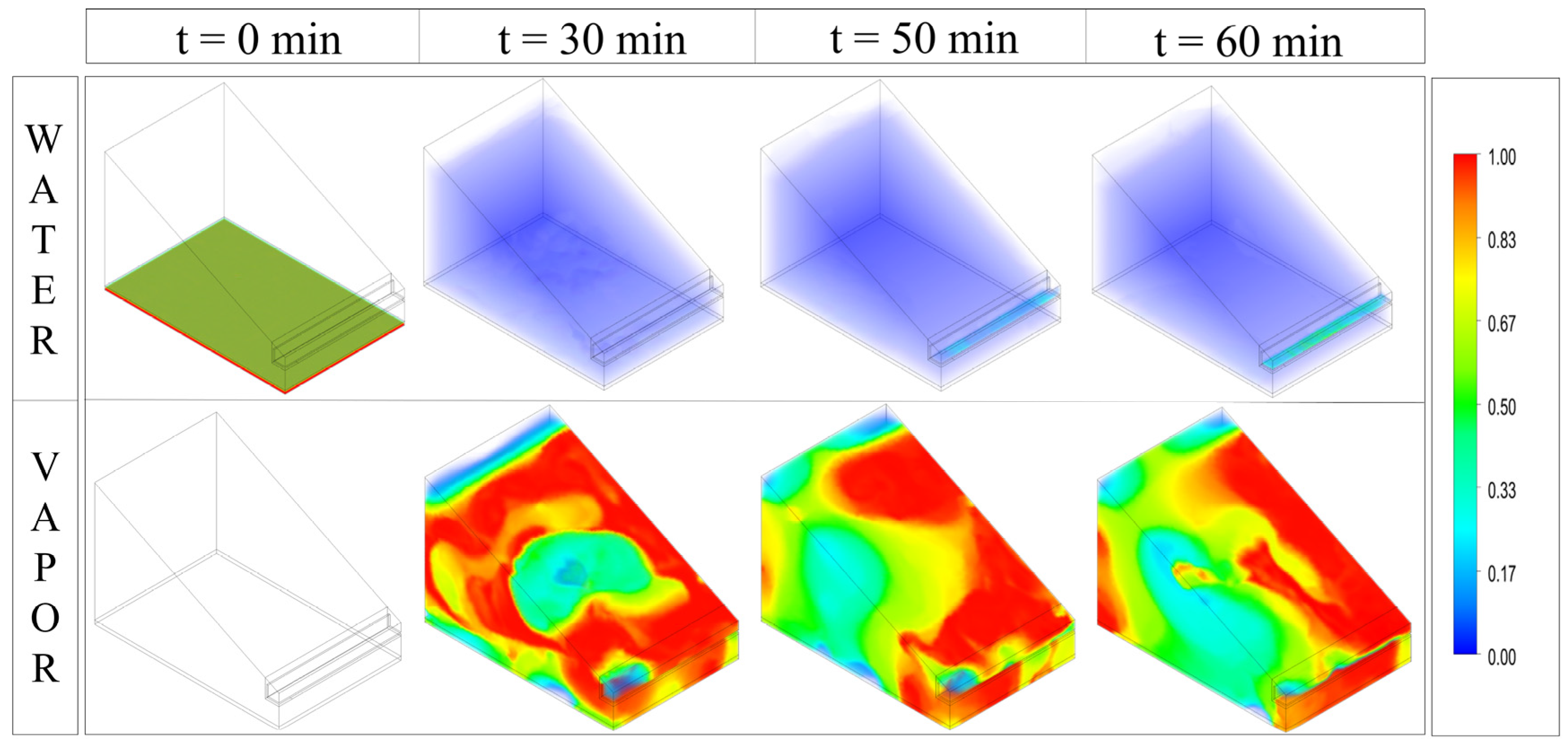
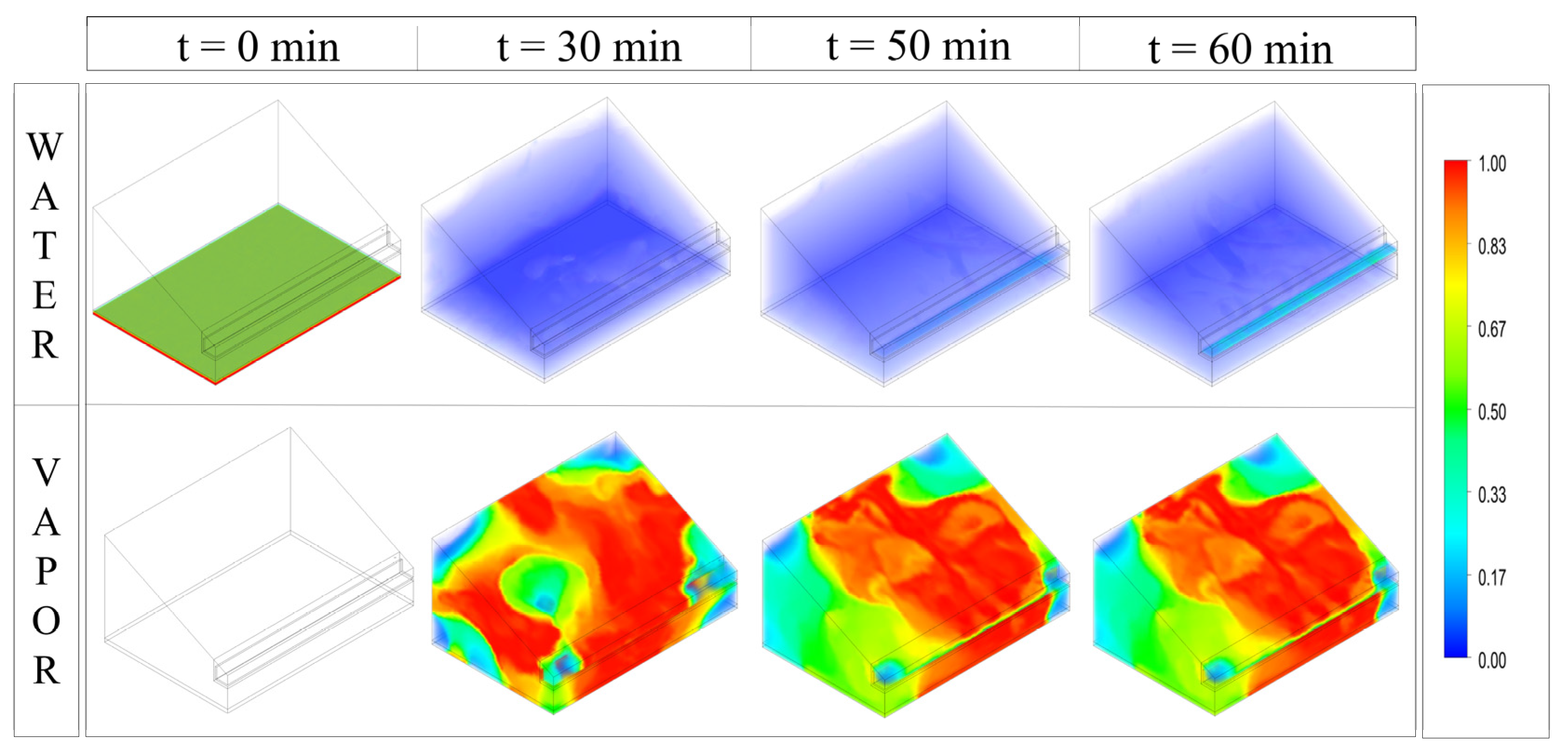
Figure 11 shows the behavior of the water volume fraction during different periods within a one-hour simulation through volume rendering, and Figure 11 shows the behavior of the vapor volume fraction. Among the main observations that can be made using the figures is the possibility to verify in the first one, the evaporation of water in the initial minutes and, afterward, the beginning of the condensation process with a part of the water volume in the flume. Figure 11 shows the behavior of the vapor fraction, allowing a comparison with Figure 11 because, with the evaporation of water, the model begins to be filled with vapor, which is the gaseous form of water and tends to fill the entire volume in which it is contained.

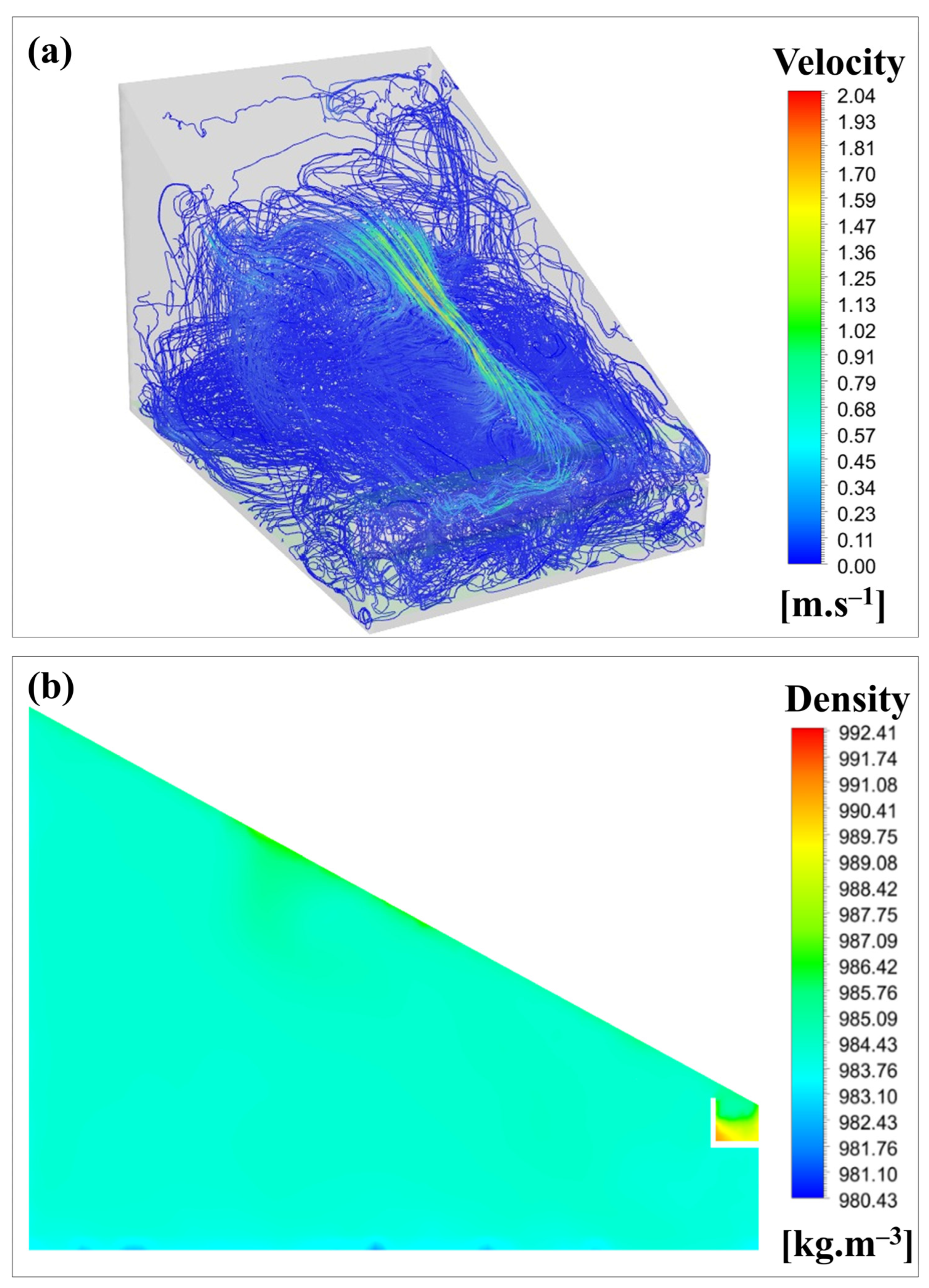
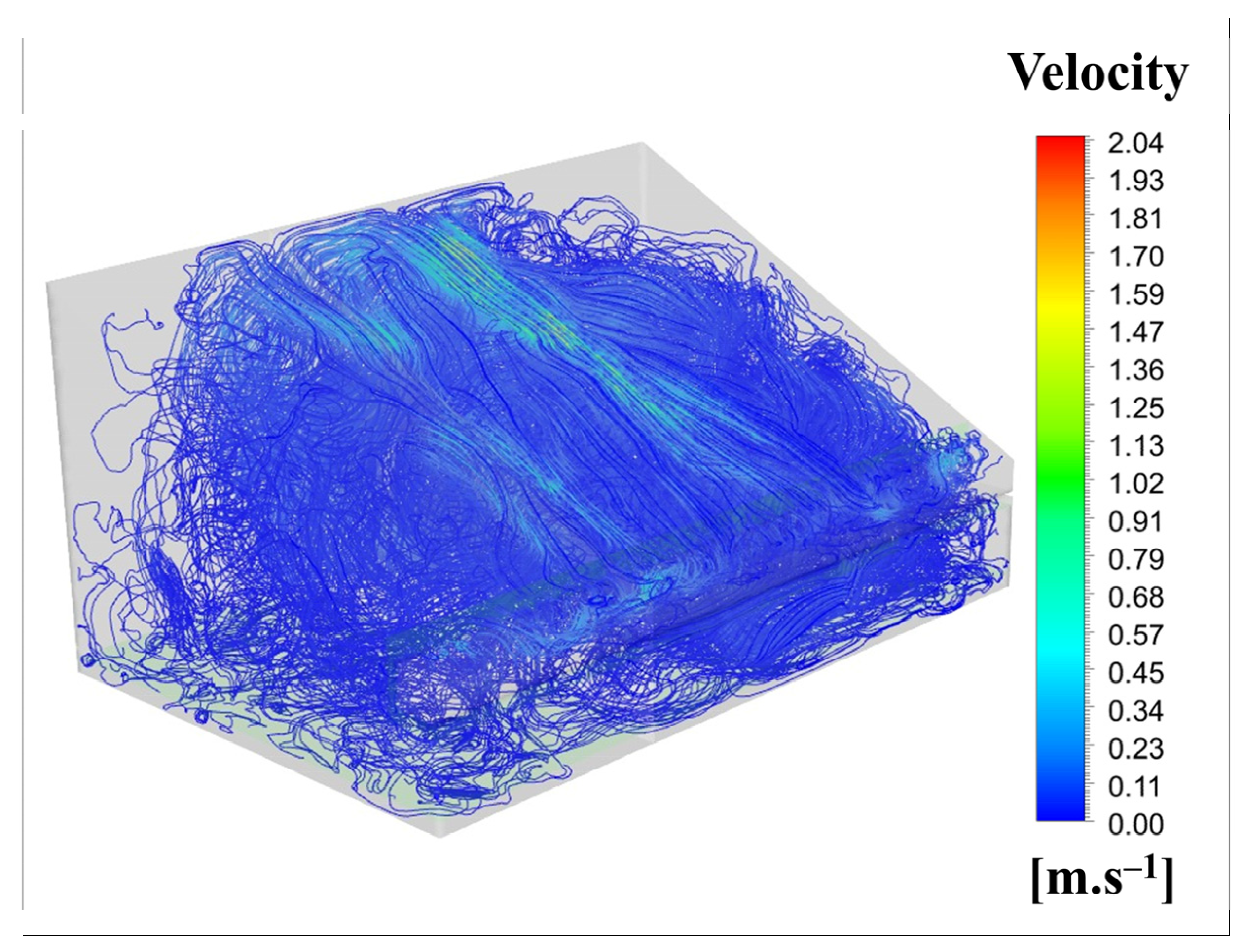
Figure 12a shows the behavior of the fluid mixing velocity for 1 h when employing streamlines. It can be observed from this figure that there are zones of recirculation and vorticity in the flow. While there are zones of higher velocities in the upper part, a zone of low velocity occurs in the middle part, and the flow shows a tendency to flow into the gutter. El-Sebaey et al. also observed this phenomenon and characterized it as a consequence of the influence of air recirculation in driving the condensed volume toward the flume [15]. As the water in the model heats up, the temperature of the fluid also varies. Figure 12b shows the density profile in an intermediate plane on the Z-axis, where it can be observed that the density profile has higher values close to the glass and trough regions. This result corroborates the physics involved in the process because a higher value for the water density is an indicator that condensation occurs in this zone, which is a direct and inherent justification for the effect of the lower temperature on the density of these zones on the temperature of the plate and the interior of the model.

3.3. Proposed Modified Model

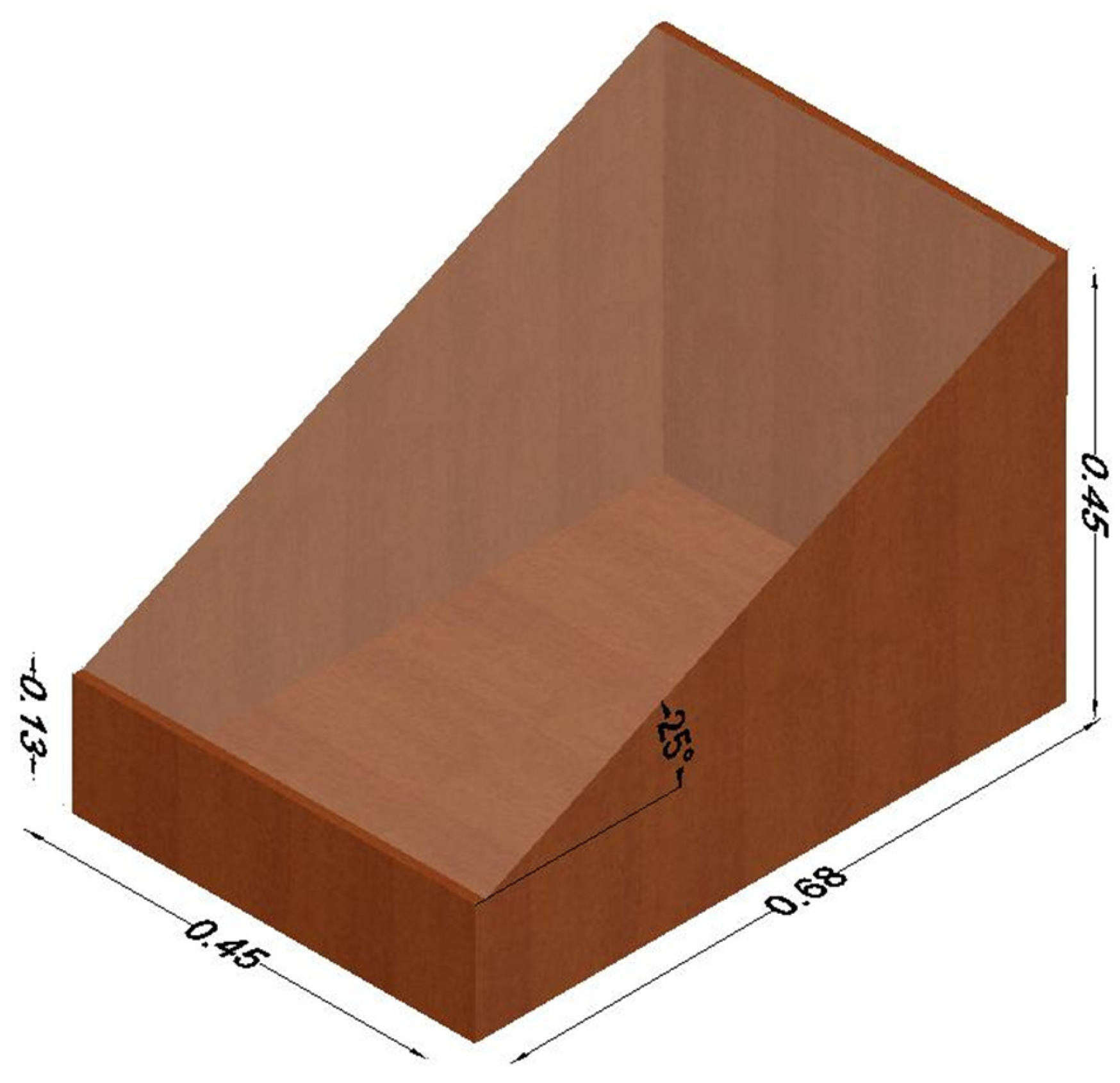
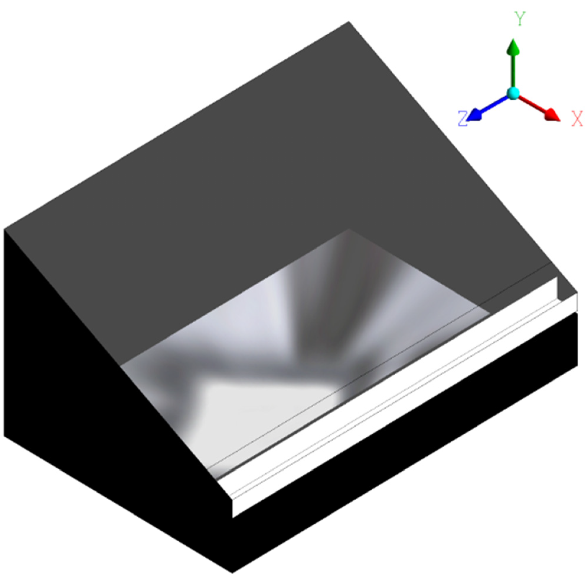
One of the several advantages of using numerical simulations is the possibility of computationally generating modifications in the models and promoting optimizations and parametric analysis. In this sense, with the observation of the variation of geometries found in the literature for solar still prototypes, a numerical simulation was performed to understand whether the horizontalization of the physical model can be more efficient than the constructed model commonly used in studies in the literature. 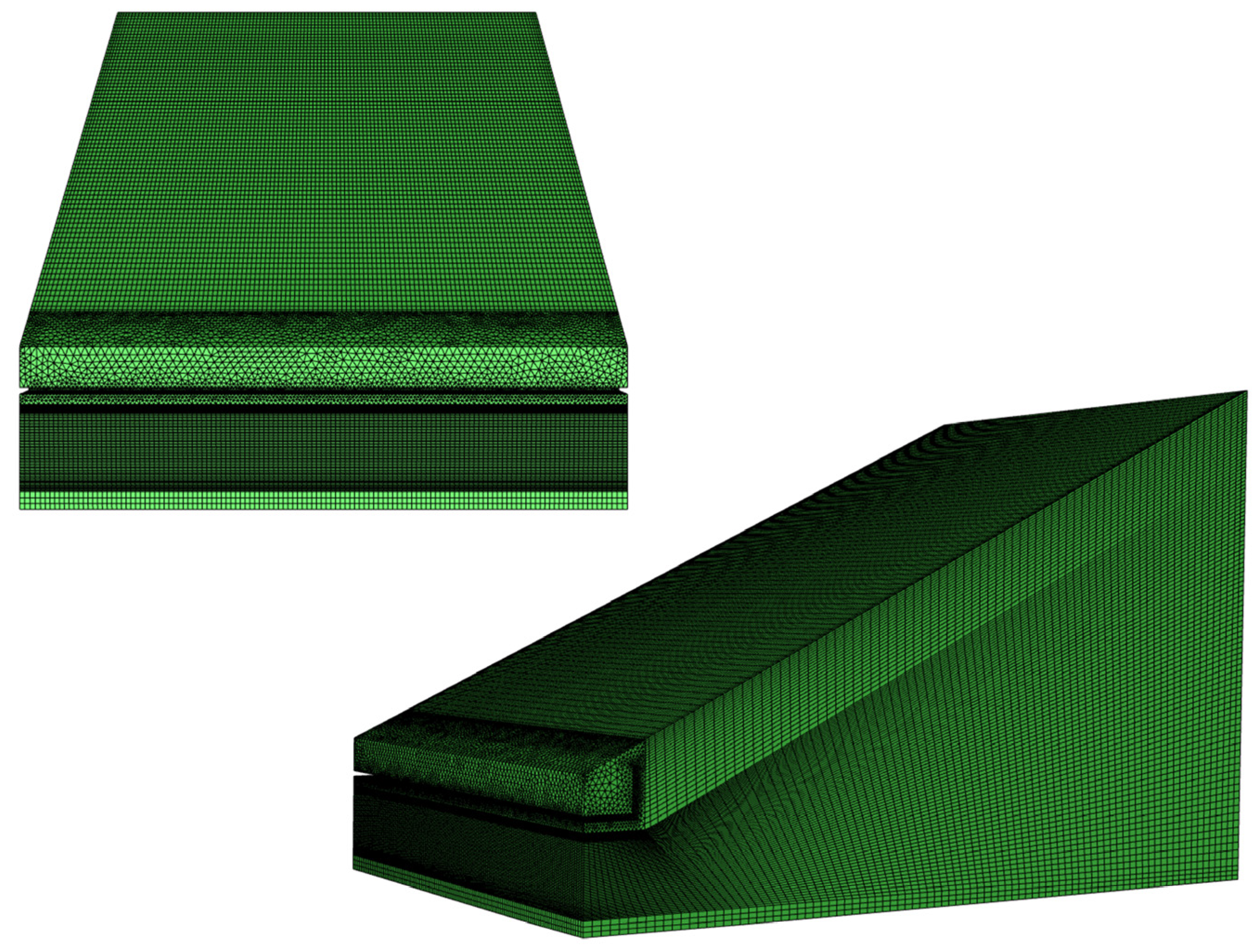Thus, the geometry of the current model underwent some modifications, where the length of the X-axis was swapped with that of the Z-axis. Therefore, the geometry was left with a width of 680 mm and a depth of 450 mm. Because the model did not undergo many changes, the mesh generated in the previous case remained at its parameters and preserved its quality. 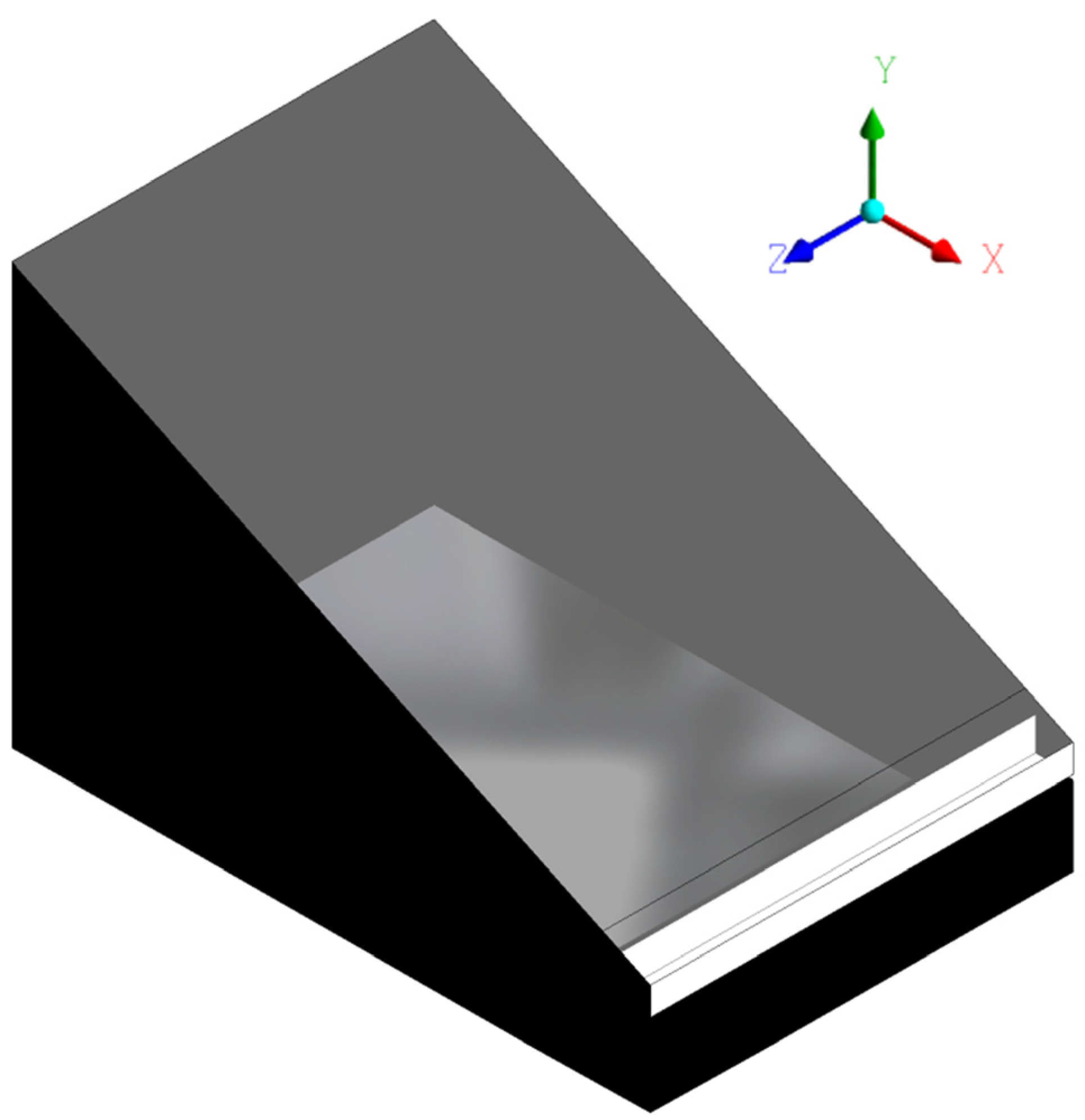Figure 13 illustrates the geometry of the model used.

The results of this model proved to be superior to those of the conventional model. The water production was 0.074 L in one hour, thus the performance was approximately 15% higher than that of the conventional model (0.071 L). Figure 14 shows the behavior of the water volume fraction over time through volume rendering and Figure 14 shows the behavior of the vapor volume fraction. Figure 14 shows a justification for the better performance of this model because as the spacing of the glass between the bottom wall and the front wall of the trough has been reduced, a higher volume of water should condense. This is because the glass in this format generates a larger area of direct contact with the vapor in the initial minutes, considering that in the previous model, the position of the glass had a lower horizontal length. In addition, the gutter has a greater horizontal length in this model, which may improve water capture. Similar to the vapor volume fraction in the previous case, in this model, the vapor behavior also occurs in a way that fills the entire domain. Figure 14 illustrates this behavior.

Figure 15 shows the velocity behavior of the horizontal model. In this image, it is evident that the behavior of higher velocity at the surface of the equipment is characteristic of desalter, as the phenomenon is similar to the previous model, and also presents regions of flow recirculation and vorticities. The regions below and close to the wall exhibited low velocities.

4. Conclusions

The current work focused on developing a simple solar still with low-cost materials that can be built by anyone, anywhere. In addition, the study presented three-dimensional multiphase CFD models for a single-slope solar still. The developed model can predict the results for any solar still without experimental data, using only local solar radiation, water flow, and equipment geometry data. The main results of this study are as follows:

• A low-cost solar still was developed using simple materials that were easily accessible to the community.
• The experimental test showed the effectiveness of the water desalination process using the built prototype. The quality of the produced water generated good results when electrical conductivity was evaluated.
• The experimental and simulated efficiencies were 12.3% and 11.8%.
• The model showed a variation in density and temperature consistent with expectations, and regarding the velocity profile, the streamlines showed several recirculation zones and a higher velocity in the upper part of the model, near the glass.
• It was found that the efficiency of the equipment increased when the tank geometry was modified, thus promoting an increase in desalination efficiency.
• The simulation results show that computational fluid dynamics is an important tool for improving the performance of the equipment.

References

1. Kumar, A. CFD Modeling and Validation of a Single Slope Solar Still. Ph.D. Thesis, Malaviya National Institute of Technology Jaipur, Jaipur, India, 2015. [Google Scholar]
2. Uzair, M.; Naqvi, A.A.; Yousuf, M.U. Numerical investigation to determine the optimal tilt angle of single slope solar still during summer season. Tecciencia 2022, 17, 29–39. [Google Scholar] [CrossRef]
3. Homaeigohar, S.; Elbahri, M. Graphene membranes for water desalination. NPG Asia Mater. 2017, 9, e427. [Google Scholar] [CrossRef]
4. Alim, M.A.; Rahman, A.; Tao, Z.; Samali, B.; Khan, M.M.; Shirin, S. Suitability of roof harvested rainwater for potential potable water production: A scoping review. J. Clean Prod. 2020, 248, 119226. [Google Scholar] [CrossRef]
5. United Nations. The Sustainable Development Goals Report; United Nations: New York, NY, USA, 2020; pp. 4–5. [Google Scholar]
6. World Water Council. Water and Climate Blue Book; World Water Council: Marseille, France, 2017; p. 48. [Google Scholar]
7. Patel, S.K.; Singh, D.; Devnani, G.L.; Sinha, S.; Singh, D. Potable water production via desalination technique using solar still integrated with partial cooling coil condenser. Sustain. Energy Technol. Assess. 2021, 43, 100927. [Google Scholar] [CrossRef]
8. Mir, N.; Bicer, Y. Integration of electrodialysis with renewable energy sources for sustainable freshwater production: A review. J. Environ. Manag. 2021, 289, 112496. [Google Scholar] [CrossRef] [PubMed]
9. Shah, K.M.; Billinge, I.H.; Chen, X.; Fan, H.; Huang, Y.; Winton, R.K.; Yip, N.Y. Drivers, challenges, and emerging technologies for desalination of high-salinity brines: A critical review. Desalination 2022, 538, 115827. [Google Scholar] [CrossRef]
10. Thakkar, H.; Sadasivuni, K.K.; Ramana, P.V.; Panchal, H.; Suresh, M.; Israr, M.; Elklawy, M.; AlmElDin, H. Comparative analysis of the use of flash evaporator and solar still with a solar desalination system. Int. J. Ambient Energy 2022, 43, 1561–1568. [Google Scholar] [CrossRef]
11. Bait, O. Direct and indirect solar–powered desalination processes loaded with nanoparticles: A review. Sustain. Energy Technol. Assess. 2020, 37, 100597. [Google Scholar] [CrossRef]
12. Manokar, A.M.; Murugavel, K.K.; Esakkimuthu, G. Different parameters affecting the rate of evaporation and condensation on passive solar still—A review. Renew. Sustain. Energy Rev. 2014, 38, 309–322. [Google Scholar] [CrossRef]
13. Cervantes-Rendón, E.; Ibarra-Bahena, J.; Cervera-Gómez, L.E.; Romero, R.J.; Cerezo, J.; Rodríguez-Martínez, A.; Dehesa-Carrasco, U. Rural Application of a Low-Pressure Reverse Osmosis Desalination System Powered by Solar–Photovoltaic Energy for Mexican Arid Zones. Sustainability 2022, 14, 10958. [Google Scholar] [CrossRef]
14. Vaithilingam, S.; Gopal, S.T.; Srinivasan, S.K.; Manokar, A.M.; Sathyamurthy, R.; Esakkimuthu, G.S.; Kumar, R.; Sharifpur, M. An extensive review on thermodynamic aspect based solar desalination techniques. J. Therm. Anal. Calorim. 2021, 145, 1103–1119. [Google Scholar] [CrossRef]
15. S. El-Sebaey, M.; Ellman, A.; Hegazy, A.; Ghonim, T. Experimental analysis and CFD modeling for conventional basin-type solar still. Energies 2020, 13, 5734. [Google Scholar] [CrossRef]
16. Suresh, C.; Shanmugan, S. Effect of water flow in a solar still using novel materials. J. Therm. Anal. Calorim. 2019, 136, 1–14. [Google Scholar] [CrossRef]
17. Kabeel, A.E.; Sathyamurthy, R.; Sharshir, S.W.; Muthumanokar, A.; Panchal, H.; Prakash, N.; Prasad, C.; Nandakumar, S.; El Kady, M.S. Effect of water depth on a novel absorber plate of pyramid solar still coated with TiO2 nano black paint. J. Clean. Prod. 2019, 213, 185–191. [Google Scholar] [CrossRef]
18. Jadidoleslami, M.; Farahbod, F. Experimental and mathematical evaluation of solar powered still equipped by nano plate as the principle stage of zero discharge desalination process. Adv. Energy Res. 2016, 4, 147. [Google Scholar] [CrossRef]
19. Essa, F.A.; Abdullah, A.S.; Omara, Z.M. Rotating discs solar still: New mechanism of desalination. J. Clean. Prod. 2020, 275, 123200. [Google Scholar] [CrossRef]
20. Khechekhouche, A.; Elsharif, N.; Kermerchou, I.; Sadoun, A. Construction and performance evaluation of a conventional solar distiller. Herit. Sustain. Develop. 2019, 1, 72–77. [Google Scholar] [CrossRef]
21. Kudish, A.I.; Gale, J.; Zarmi, Y. A low cost design solar desalination unit. Energy Convers. Manag. 1982, 22, 269–274. [Google Scholar] [CrossRef]
22. Piekarski, C.M.; de Francisco, A.C.; da Luz, L.M.; Kovaleski, J.L.; Silva, D.A.L. Life cycle assessment of medium-density fiberboard (MDF) manufacturing process in Brazil. Sci. Total Environ. 2017, 575, 103–111. [Google Scholar] [CrossRef]
23. Taghiyari, H.R.; Ghorbanali, M.; Tahir, P.M. Effects of the improvement in thermal conductivity coefficient by nano-wollastonite on physical and mechanical properties in medium-density fiberboard (MDF). BioResources 2014, 9, 4138–4149. [Google Scholar] [CrossRef] [Green Version]
24. Zhou, L.; Yuan, T.B.; Yang, X.S.; Liu, Z.Y.; Wang, Q.Z.; Xiao, B.L.; Ma, Z.Y. Micro-scale prediction of effective thermal conductivity of CNT/Al composites by finite element method. Int. J. Therm. Sci. 2022, 171, 107206. [Google Scholar] [CrossRef]
25. Millero, F.J.; Feistel, R.; Wright, D.G.; McDougall, T.J. The composition of Standard Seawater and the definition of the Reference-Composition Salinity Scale. Deep Sea Res. Part I Oceanogr. Res. Pap. 2008, 55, 50–72. [Google Scholar] [CrossRef]
26. Doornbusch, G.; van der Wal, M.; Tedesco, M.; Post, J.; Nijmeijer, K.; Borneman, Z. Multistage electrodialysis for desalination of natural seawater. Desalination 2021, 505, 114973. [Google Scholar] [CrossRef]
27. Shalev, N.; Lazar, B.; Köbberich, M.; Halicz, L.; Gavrieli, I. The chemical evolution of brine and Mg-K-salts along the course of extreme evaporation of seawater–an experimental study. Geochim. Cosmochim. Acta. 2018, 241, 164–179. [Google Scholar] [CrossRef]
28. Tyler, R.H.; Boyer, T.P.; Minami, T.; Zweng, M.M.; Reagan, J.R. Electrical conductivity of the global ocean. Earth Planets Space 2017, 69, 1–10. [Google Scholar] [CrossRef]
29. Zheng, Z.; Fu, Y.; Liu, K.; Xiao, R.; Wang, X.; Shi, H. Three-stage vertical distribution of seawater conductivity. Sci. Rep. 2018, 8, 9916. [Google Scholar] [CrossRef]
30. Badran, O.O.; Abu-Khader, M.M. Evaluating thermal performance of a single slope solar still. Heat Mass Transf. 2007, 43, 985–995. [Google Scholar] [CrossRef]
31. Akram, M.W.; Motin, S.A.; Hoque, M.A.; Mustafi, N.N. Design, construction and performance test of a solar still for water desalination in Bangladesh perspective. In AIP Conference Proceedings; AIP Publishing LLC: Dhaka, Bangladesh, 2019. [Google Scholar]
32. Ansys, I. Module 05: Mesh Quality & Advanced Topics. 2016. [Google Scholar]
33. Rahman, M.M.; Öztop, H.F.; Ahsan, A.; Kalam, M.A.; Varol, Y. Double-diffusive natural convection in a triangular solar collector. Int. Commun. Heat Mass Transf. 2021, 39, 264–269. [Google Scholar] [CrossRef]
34. Boiko, A.V.; Kirilovskiy, S.V.; Maslov, A.A.; Poplavskaya, T.V. Engineering modeling of the laminar–turbulent transition: Achievements and problems. J. Appl. Mech. Tech. Phys. 2015, 56, 761–776. [Google Scholar] [CrossRef]
35. Launder, B.E.; Spalding, D.B. Lectures in Mathematical Models of Turbulence, 1st ed.; Academic Press: Cambridge, MA, USA, 1972; 169p. [Google Scholar]
36. Hanjalić, K. Advanced turbulence closure models: A view of current status and future prospects. Int. J. Heat Fluid Flow 1994, 15, 178–203. [Google Scholar] [CrossRef]
37. Lien, F.S.; Leschziner, M.A. Assessment of turbulence-transport models including non-linear RNG eddy-viscosity formulation and second-moment closure for flow over a backward-facing step. Comput. Fluids 1994, 23, 983–1004. [Google Scholar] [CrossRef]
38. Yakhot, V.; Orszag, S.A. Renormalization group analysis of turbulence. I. Basic theory. J. Sci. Comput. 1986, 1, 3–51. [Google Scholar] [CrossRef]
39. Yan, B.W.; Li, Q.S.; He, Y.C.; Chan, P.W. RANS simulation of neutral atmospheric boundary layer flows over complex terrain by proper imposition of boundary conditions and modification on the k-ε model. Environ. Fluid Mech. 2016, 16, 1–23. [Google Scholar] [CrossRef]
40. Keshtkar, M.; Eslami, M.; Jafarpur, K. A novel procedure for transient CFD modeling of basin solar stills: Coupling of species and energy equations. Desalination 2020, 481, 114350. [Google Scholar] [CrossRef]
41. Hossain, M.S.; Hossain, M.I.; Pramanik, S.; Ahamed, J.U. Analyzing the Turbulent Flow Characteristics by Utilizing k-ε Turbulence Model. European J. Adv. Eng. Technol. 2017, 2, 28–34. [Google Scholar] [CrossRef]
42. Lee, W.H. A Pressure Iteration Scheme for Two-phase Flow Modeling. In Multiphase Transport. Fundamentals, Reactor Safety, Applications; Veziroglu, T.N., Ed.; Hemisphere Publishing: Washington, DC, USA, 1980; pp. 407–432. [Google Scholar]
43. Kharangate, C.R.; Mudawar, I. Review of computational studies on boiling and condensation. Int. J. Heat Mass Transf. 2017, 108, 1164–1196. [Google Scholar] [CrossRef]
44. Rajaseenivasan, T.; Elango, T.; Murugavel, K.K. Comparative study of double basin and single basin solar stills. Desalination 2013, 309, 27–31. [Google Scholar] [CrossRef]
45. Kikuda, R.; Pereira Gomes, R.; Rodrigues Gama, A.; De Paula Silva, J.A.; Pereira Dos Santos, A.; Rodrigues Alves, K.; Nascimento Arruda, P.; Scalize, P.S.; Gonçalves Vieira, J.D.; Carneiro, L.C.; et al. Evaluation of Water Quality of Buritis Lake. Water 2022, 14, 1414. [Google Scholar] [CrossRef]
46. Meride, Y.; Ayenew, B. Drinking water quality assessment and its effects on residents health in Wondo genet campus, Ethiopia. Environ. Syst. Res. 2016, 5, 1–7. [Google Scholar] [CrossRef]
47. Purnachandrakumar, D.; Mittal, G.; Sharma, R.K.; Singh, D.B.; Tiwari, S.; Sinhmar, H. Review on performance assessment of solar stills using computational fluid dynamics (CFD). Environ. Sci. Pollut. Res. 2022, 29, 38673–38714. [Google Scholar] [CrossRef] [PubMed]
Figure 1. Dimensions in meters of the solar still structure.
Eng 04 00023 g001
Figure 2. Process of building the solar still. The sequence is described in the text.
Eng 04 00023 g002
Figure 3. The geometry of the virtual model of the solar still.
Eng 04 00023 g003
Figure 4. The 3D elements for Grid 2: front view and side view.
Eng 04 00023 g004
Figure 5. Desalinated water production and efficiency.
Eng 04 00023 g005
Figure 6. (a) Average global radiation (W/m2). (b) Accumulative water volume.
Eng 04 00023 g006
Figure 7. Desalinated water and temperatures for tests (a) 1; (b) 2; (c) 3; and (d) 4.
Eng 04 00023 g007
Figure 8. Electrical conductivity of the water obtained with the solar still.
Eng 04 00023 g008
Figure 9. Comparison of the numerical and experimental model.
Eng 04 00023 g009
Figure 10. Temperature profile over the analysis time (a) 0; (b) 30; (c) 50; and (d) 60 min.
Eng 04 00023 g010
Figure 11. A volumetric fraction over time with volume rendering of water and vapor.
Eng 04 00023 g011
Figure 12. (a) Mixing velocity for the 1 h time using streamlines. (b) Density profile in an intermediate plane on the Z-axis at 1 h.
Eng 04 00023 g012
Figure 13. New horizontal geometry model.
Eng 04 00023 g013
Figure 14. A volumetric fraction over time with volume rendering of water and vapor.
Eng 04 00023 g014
Figure 15. Mixing velocity for the 1 h time using streamlines for the proposed model.
Eng 04 00023 g015