Kinetic Modelling for Hydrothermal Conversion of Food Wastes

Abstract

A kinetic model was developed for the prediction of HTL product yields based on a chemical mechanism. The model was developed after experimental studies on food wastes and food processing wastes. The model parameters were determined by training the model on experimental data on HTL of food wastes. Two other models from the literature were also tested. The calculated yields were compared with a large range of experimental data from the literature. Yields of bio-oil and char can be predicted from the process conditions, temperature, holding time, dry matter content, and the biochemical composition of the resource. Differences in the experimental recovery procedure and polarity of the extraction solvent are taken into account. This study shows that a kinetic model based on compositions allows a more detailed representation of the hydrothermal reactions than models purely based on resources and products. The precision of any model remains, however, largely dependent on the quality of the input data.

1. Introduction

Food wastes represent an interesting resource that can be found in every European city, from canteens, restaurants, and households to agricultural products transformation plants. In Europe, approximately 50 MT of food waste is produced each year [1], not counting residues from the food processing industry. This resource can contribute effectively to the need for alternative biofuels with even a carbon negative balance for the global process route, hence reducing the global warming effect of mobility [2,3]. As an example of the valorisation of dry and wet wastes, the European project Waste2Road aims to develop conversion pathways to produce biofuels from various wastes. Among the possibilities, hydrothermal liquefaction is considered as a serious way to valorise food waste [4].

Hydrothermal liquefaction (HTL) is a process that is still under development [5]. It is particularly adapted for the conversion of wet organic resources due to the fact that the contained water is also the conversion medium, acting as a solvent but also as a reactant. The biochemical biomass compounds under hot compressed water are converted into a biocrude. This biocrude is an oily material containing bio-oil and char. The hydrothermal conversion takes place at temperatures between 300 and 400 °C and at pressures above the saturation pressure to ensure that water remains in the liquid phase, typically above 100 bar [6]. Under these conditions, the ionisation of water increases while its polarity decreases, favouring depolymerisation and dehydration of biomass biopolymers to produce hydrophobic compounds [7]. Previous work on HTL of agro-industrial residues has shown that the biochemical composition of the initial matter is the major parameter influencing conversion efficiency and quality of the product [8]. Prediction of bio-oil yields can be done by linear or polynomial equation with a parameters determination obtained by a design of experiment [9], but this kind of modelling is difficult to extrapolate to a wide range of biomass resources and even more difficult if the biochemical composition of the wastes is variable. This is especially the case when dealing with wastes collected at different locations and during different seasons.

Modelling with machine learning algorithms is becoming popular in the HTL community [10,11,12,13]. These modelling techniques are generalisations of the before mentioned linear or polynomial models. These techniques can be very powerful and allow relatively accurate prediction of the results. In addition, they can also contribute to the understanding of the conversion from a global statistical perspective [6]. Machine learning techniques have many advantages above simplified polynomial models, but cannot really contribute to the knowledge of the underlying chemistry. They offer the advantage of a high accuracy and predictability if all parameters of influence have been considered.

Kinetic modelling promises both reliable predictions as well as an insight to the underlying chemistry. The approach is limited by the complexity of the chemistry. For now, it is impossible to fully characterise the resource, identify all reaction products and intermediaries, and identify all underlying reactions. Initial attempts of kinetic models concentrate on a global biomass characterisation and include simple reactions to final products, characterised by their phases; generally, bio-oil, solids, aqueous phase, and gas. These models were pioneered by Valdez et al. [14,15] and later reused by other authors [16,17]. Other reaction schemes have been proposed by Obeid et al. [18,19] and Qian et al. [20]. Hietala et al. [21] also proposed a simplified model before publishing a more detailed kinetic model specific to microalgae [22]. A lot of work in characterization of the biomass and identification and quantification of compounds or reaction schemes still needs to be done to improve the underlying knowledge and the predictability of the kinetic models.

There is a need for a deeper understanding of the chemical conversion routes, allowing for a more precise model. A more universal model based on a large experimental database used for model training can assure a more universal quality. The objective of this work is to develop a model able to predict HTL products yields in relation with the initial biomass biochemical composition and the process conditions. A new chemical mechanism is proposed and used for the building of a new kinetic model following the work of Briand [23]. The experimental database is based on HTL batch experiments following the usual experimental procedure in addition to data gathered from the literature for the same kind of resource, the food wastes. The dataset is partly published and described in [6,24] and is supplied as Supplementary Material.

2. Material and Methods

2.1. Resources

A variety of food wastes have been selected and converted. They were characterized by moisture content, ash content, and proximate and ultimate analyses. Proximate and ultimate analysis of resources were subcontracted to the commercial laboratories SOCOR and CAPINOV. Results of the analyses are given in

Table 1. Feedstock characteristics.

		BCP	BSG	FW2	FFOM	DFOR
Feedstock Origin		Les Vergers Boiron	La Brasserie Du Dauphiné	CEA Restaurant H1	Suez France	EGE
Total moisture. as received	wt%	52.5	72.5	82	50	42
Ash 550 °C, dry matter	wt%	3.7 ± 0.3	3.0 ± 0.2	4.8 ± 0.3	22.5	28
Carbon, dry matter	wt%	48.7 ± 0.7	44.7 ± 0.3	43.8 ± 0.2	37.7	37.6
Hydrogen, dry matter	wt%	6.5 ± 0.1	6.6 ± 0,1	8.1 ± 0.1	5.2	5.9
Nitrogen, dry matter	wt%	2.8 ± 0.1	2.8 ± 0.1	3.2 ± 0.5	1.7	4.8
Sulfur, dry matter	wt%	0.2 ± 0.1	0.2 ± 0.1	0.2 ± 0.3	0.3	0.5
Cellulose, dry ash free	wt%	16.0	11.5	7.7	30.1	8.8
Hemicellulose, dry ash free	wt%	15.1	30.1	12.5	5.5	9.8
Lignin, dry ash free	wt%	16.5	3.3	2.8	7.5	24.2
Sugars, dry ash free	wt%	9.6	26.0	40.1	13	0
Proteins, dry ash free	wt%	18.4	19.9	6.5	9.6	29.5
Lipids, dry ash free	wt%	20.7	6.2	11.5	3.8	1.3

. Even if the elemental analyses look similar, the biochemical composition of those two resources are quite different, except for their protein content. Blackcurrant pomace (BCP) is a residue of juice production and was sourced from “Les Vergers de Boiron” in Valence, France. Brewers’ Spent Grains (BSG) were sourced from “La Brasserie du Dauphiné” near Grenoble, France. Food wastes were collected in batches from the waste disposal of the CEA campus restaurant H1 during a three month period. Three separate campaigns collected three food waste batches. This study concentrates on the second batch (FW2). The fermentable fraction of organic municipal waste (FFOM) is the product of the mechanical separation of household waste to produce the feedstock for the methanisation plant, and was supplied by Suez in Montpellier, France. The digested fermentable fraction of organic residue (DFOR) is produced from household waste at the methanisation plant of Energi Gjenvinnings Etatens (EGE), the waste valorisation company of the city of Oslo in Norway. Biochemical compositions and ash content constitute, with temperature and residence time, the input data for the predictive model.

Food wastes have a variable composition depending on the restaurant menu, but generally have a low lignin content. DFOR and FFOM are rich in ash and low in lipids.

2.2. Experimental Procedure

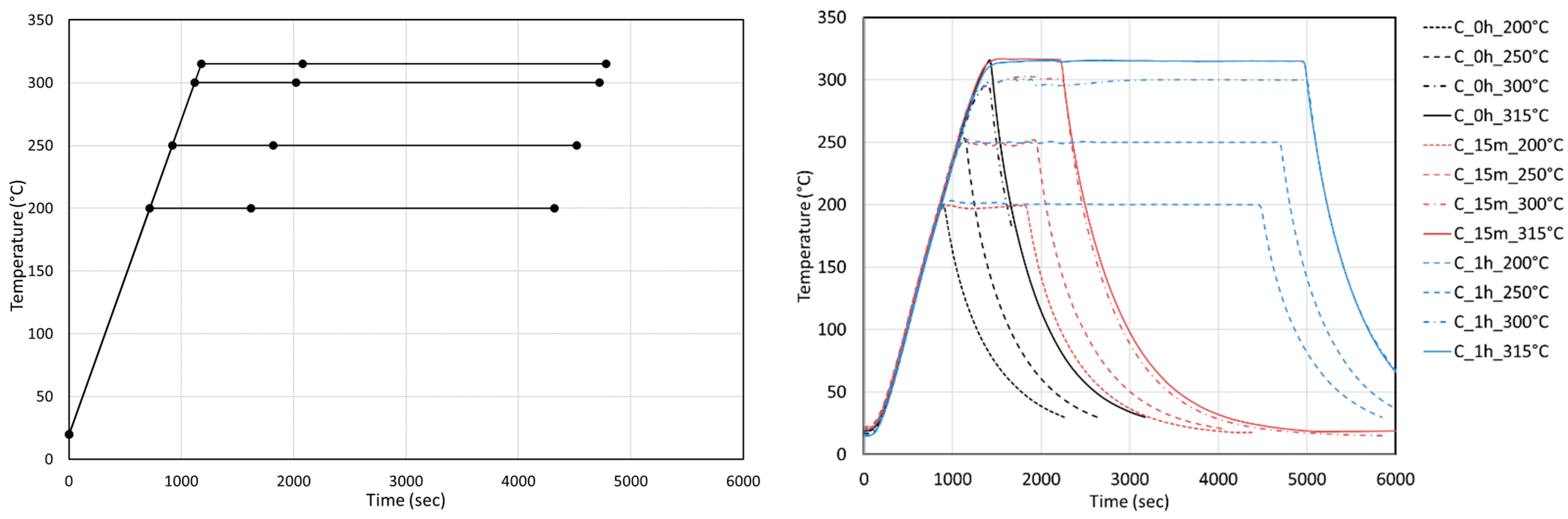
Experiments were performed in a batch reactor of 600 mL volume with different resources, food wastes, and agro-industrial resources. The resource to water mixture ratio was kept constant at 1:9 in all experiments. Experiments were performed using always the same programmed linear heat-up ramp of 15 °C/min in order to have reproducible conditions. The experimental temperature conditions for the experiments on blackcurrant pomace and brewers’ spent grains are depicted in the Figure 1, with 200, 250, 300, and 315 °C and holding times of 0, 15, and 60 min. The experiments at holding time 0 min can be considered as intermediary points during the heat-up ramp of experiments at higher temperatures. As can be seen from Figure 1, the set point ramp is well-respected by the temperature controller. There is a small constant time delay due to the inertia of the heater.

For other resources (FW2, FFOM, and DFOR), the experimental conditions were less structured. The temperatures were 200, 250, 300, 325, and 350 °C with holding times 0 and 30 min. The same programmed linear temperature ramp of 15 °C/min was applied in most cases unless otherwise stated with the experiment.

At the end of the desired residence time, the reactor is rapidly cooled down to room temperature. Final pressure is registered for the gas production calculation, and the gas is vented after sampling for gas composition analysis by a µGC. The solvent is not poured directly into the reactor, but the liquid product is poured onto a filter to separate the aqueous phase from the raw biocrudes product. This raw product, called biocrude, is dried at 105 °C until at a stable weight. The oil content of the dried raw biocrude, called “biocrude,” is determined by solvent extraction with ethyl acetate or other solvents. More details on the experimental methods can be found in previous work [6,25].

2.3. Yield Calculations

The yields of the different products are always presented as a fraction of the dry matter feed. Hydrothermal liquefaction yields three different phases: an aqueous phase with dissolved organics, biocrude containing the bio-oil char, and a gaseous phase mainly constituting of carbon dioxide. Biocrudes are complex mixtures containing an oily and a solid fraction. Biocrude is the raw product obtained after the hydrothermal transformation, and it is sometimes referred to as bio-oil or raw residue. Biocrude can be a fluid oil with little or no char, but can also be a solid with little or no oil. This largely depends on the resource and conditions. The solid fraction is, in fact, an insoluble fraction in a determined solvent. In this work, the biochar fraction X_char (-) in the biocrude is determined after extraction with ethyl acetate as the solvent. The yield of biocrude Y_bc (-) is the weight of dry biocrude W_bc (g) divided by the initial weight of dry matter entered into the reactor, and the yield of biochar ($Y_{char})$ is the weight of biochar divided by the initial weight of dry matter DM (g), Equation (1). The bio-oil yield ($Y_{bio-oil})$ is calculated by difference as given by Equation (2):

$$Y_{char}=\frac{\left(W_{BC}·X_{char}\right)}{DM}$$

(1)

$$Y_{bio-oil}=Y_{bc}-Y_{char}$$

(2)

The gas yield Y_gas (-) is determined by calculation of the gas produced by using the initial pressure value P_i (Pa) at the initial temperature T_i (K) and the final pressure value P_f (Pa) in the reactor at final temperature T_f (K) after cooling, with the ideal gas law. In addition, the quantity of CO₂ dissolved in the aqueous phase in the final conditions W_CO2diss (g) is calculated with Henry’s law [25], Equation (3).

$$Y_{gas}=\frac{Mw·\frac{\left(V_R-V_L\right)}{R}·\left(\frac{P_f}{T_f}-\frac{P_i}{T_i}\right)+W_{CO2\_Diss}}{DM}$$

(3)

With V_R (L): reactor volume, V_L (L): volume of liquid in the reactor, R (J·K⁻¹·mol⁻¹): the gas constant, and Mw (g·mol⁻¹): the average molecular weight of the produced gas.

The yield of dissolved organics in the aqueous phase ($Y_{AP}$) is estimated by difference, Equation (4).

$$Y_{AP}=100\%-Y_{char}-Y_{bio-oil}-Y_{gas}$$

(4)

2.4. Description of the Dataset

The dataset and experimental methods used in this study are described in previous work [6,24] as well as the supplemental data associated to this paper. This dataset is the result of experiments at the CEA laboratory and a literature study. Various experiments on a wide variety of food wastes at different temperatures and holding times were included. Data from Motavaf et al. [26], Bayat et al. [27], Aierzhati et al. [28], Evcil et al. [29], Yang et al. [30,31,32,33], and Déniel [34] are also included. It should be noted that Motavaf, Aierzhati, and Evcil do not present data for char yield, only bio-oil.

Weights are applied to the data. Experiments (lines in the data file) have a weight variable associated. Some of these experiments are the average of multiple experiments and are therefore more reliable. These experiments have a more important weight in the error function. In the same way, weights are applied to products. As the oil is the main product of interest, it has a weight factor of 3. The weights associated to the char and gas are 2 and 1, respectively. In most published studies, the gas yield is calculated from the pressure increase, not including dissolved CO₂. It is therefore not a very accurate value. The water phase is mostly calculated by difference in most published data and cannot be considered reliable information to fit a model. Missing yields from studies have a zero weight applied, and are therefore not taken into account in the error calculation and the model fitting. The model can be trained to a set of experimental data in the database, filtered for an author, a resource type, or a random selection of the data.

3. Model Development

Different kinetic models have been coded in a Python program using generic solver algorithms. The program includes the models described by Valdez et al. [14] and Obeid et al. [18], as well as the model described in this paper. Given proper conditions, reactants and intermediary products are supposed to react to form products with rates formulated as differential equations. Kinetic modelling is essentially solving a system of ordinary differential equations with a Runge Kutta type solver. To minimise the error between the experimental data and the model results, an optimiser from the same library is used.

The reaction rate is proportional to the concentrations of the reactants multiplied by a rate constant. Each rate constant k (s⁻¹) is described by an Arrhenius expression that takes the following commonly used general form, Equation (5).

$$k=A·T^n·e^{\frac{-Ea}{RT}}$$

(5)

Here, A (units depend on the reaction) is the pre-exponential term; T (K) is temperature; Ea (J·mol⁻¹) is the activation energy; and R (J·K⁻¹·mol⁻¹) is the gas constant. It is customary to work with a molar activation energy even though all equations are mass-based. The exponent n is often taken as zero, as is the case in the current study, reducing the equation to the classic formulation by Arrhenius. The heating rates are extremely variable in the literature, varying from 10 to 100 °C·min⁻¹. For each experiment in the database, the heating rate and the type of heating profile is given. Experiments presented in this paper are mostly done with a linear temperature ramp (Equation (6)). A quadratic function approximately describes most other experiments (Equation (7)). The general kinetic system, an array of concentrations, and its derivatives is a function of time. The temperature (T, °C) at each time (t, sec) is calculated from the heating profile, the heating rate (HR, °C·min⁻¹), and the time (tsp) to reach the temperature set point (Tsp).

$$T=min\left(Tsp, Tamb+HR·t\right)$$

(6)

$$T=\min \left(Tsp, Tamb+2·HR·t-\frac{Tsp-Tamb}{ts{p}^2}·t^2\right)$$

(7)

Each reaction system has its own species that take part in the reactions or as products. Species include constituents of the biomass, intermediate species, or final products such as char or bio-oil. In the case where the chemistry is detailed with intermediate species, the final products are formed by combining the species. For species that can be present in more than one product, the distribution is modulated with the solvent polarity and extraction order.

The numerical methods in this work are drawn from the SciPy library [35] and implemented in a Python program. The ordinary differential equations of the reactions are calculated with the solve_ivp ordinary differential equation solver. The model is fitted to the experimental data in a Python program using the minize optimiser function. Pre-exponential factors and activation energy form the result for each reaction.

As a measurement of the quality of the fit, the coefficient of determination is used as calculated by the function r2_score in the SciPy library, often referred to as R², a measure that resumes the variance explained by the model divided by the total variance according to Equation (8). In this equation, ${\widehat{y}}_i$ is the predicted value for each measured value $y_i$. The average of the measured values is $\overline{y}$.

$$R^2=1-\frac{{{\displaystyle \sum }}_{i=1}^n{\left(y_i-{\widehat{y}}_i\right)}^2}{{{\displaystyle \sum }}_{i=1}^n{\left(y_i-\overline{y}\right)}^2}$$

(8)

This formulation of R² ensures that the upper limit is 1 for a perfect fit. The value 0 means a null model that is essentially a horizontal line characterized only by the intercept. Negative values are possible without limit, as a model can be arbitrarily bad.

3.1. Models from the Literature

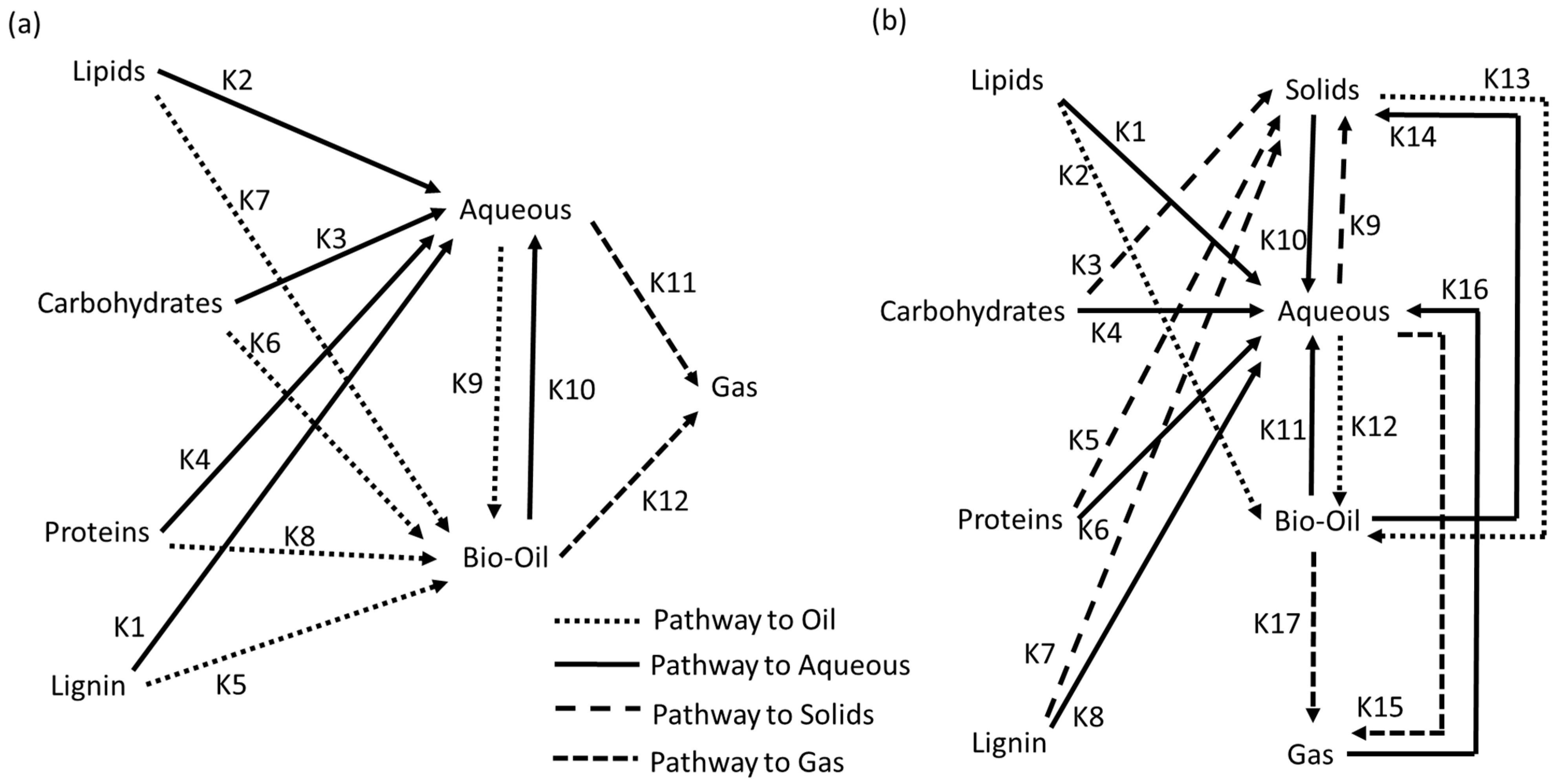
The models of Valdez et al. [14] and Obeid et al. [18,19] are shown in Figure 2 and have been coded and fitted to the data. The model from Valdez was extended with a lignin reaction path not included in the original formulation. The models only distinguish final products. Unreacted resources are qualified as solids, and this is especially important for the Valdez model.

These models are relatively simple to implement, but they lack the ability to adapt to the polarity of solvents used in the product separation. Variants of these models as well as alternative models have been formulated and published in recent years.

Valdez et al. [14] do not present pre-exponential factors and activation energies for the model, and the same group did publish Arrhenius parameters in other papers, such as for micro-algae [17]. In addition, the model as used here was extended with a lignin degradation mechanism. Obeid et al. [18,19] present sets of Arrhenius parameters for four different resources, showing the difficulties of finding a precise set to fit all resources.

3.2. Proposed Model

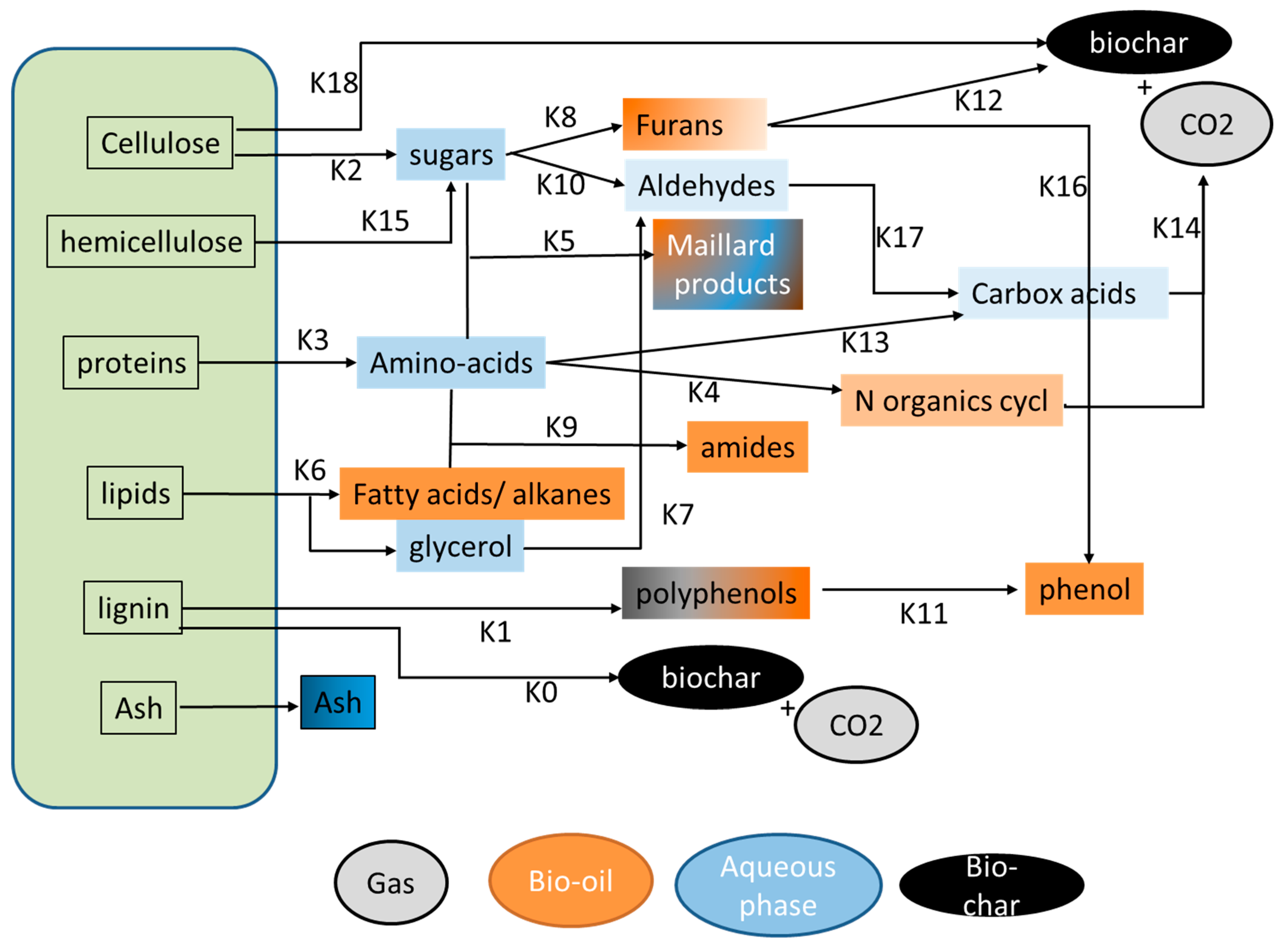
The new model proposed in this study is based on the identification of molecules in the light fraction of biocrude oil and in the aqueous phase that was done by gas chromatography coupled with mass spectrometry, as described previous work [6,8,23]. The model is based on the identification of lumped intermediary species to form a global conversion mechanism from the resource to the final product. The model is presented in Figure 3.

The kinetic model is based on a set of simplified reactions with kinetic constants expressed as Arrhenius terms (pre-exponential coefficient and activation energy). The reactions are expressed on a mass basis in g/L. The resources’ biochemical analysis forms the starting point. The temperature is ramped up to the reaction temperature using the heating rate specified for each experiment. The temperature is then held constant for the holding time. Each experiment is calculated in terms of chemical composition. The products are calculated by attributing the different compounds to the products. The produced gas is supposed to be CO₂ and is only affected to the gas phase. Some compounds are distributed between two different phases. Examples of these are poly-phenolics found in the bio-oil and supposed to be found in the char. Phenolics (phenol, gaïacol, etc.) are found in the bio-oil and in the aqueous phase. Coefficients are set up based on the extraction procedure and corrected depending on the polarity of the solvent used. The reactions that are taken into account are listed in

Table 2. List of simplified reactions used in the model.

Reaction	Reactants	Type of Reaction	Reaction Rate	Products
-	Ash	No reaction	-	Ash
0	Lignin	Hydrolysis	K0	Char + CO2
1	Lignin	Charification	K1	Polyphenolics
2	Cellulose	Hydrolysis	K2	Sugars
3	Proteins	Hydrolysis	K3	Amino acids
4	Amino acids	Dehydration/decarboxylation	K4	Nitrogenous heterocycles
5	Amino acids + Sugars	Maillard reaction	K5	Maillard compounds
6	Lipids	Hydrolysis	K6	Glycerol + Fatty acids/Alkanes
7	Glycerol	Dehydration	K7	Aldehydes
8	Sugars	Dehydration	K8	Furans
9	Amino acids + Fatty acids	Combination	K9	Amides
10	Sugars	Retro-Aldolisation	K10	Aldehyde
11	Polyphenolics	Hydrolysis	K11	Phenolics
12	Furans	Condensation	K12	Char + CO2
13	Amino acids	Deamination	K13	Carboxylic acids
14	Carboxylic acids	Decarboxylation	K14	CO2
14	Nitrogenous heterocycles	Decarboxylation	K14	CO2
15	Hemicellulose	Hydrolysis	K15	Sugars
16	Furans	Dehydration	K16	Phenolics
17	Aldehydes	Hydration	K17	Carboxylic acids
18	Cellulose	Condensation	K18	Char + CO2

.

The compounds used in the model are presented in

Table 3. List of compounds used in the model and their initial distribution factors for ethyl acetate as the solvent.

Reactants	Oil Phase	Char/Solid Phase	Gas Phase	Aqueous Phase
Ash	-	0.7	-	0.3
Lignin	-	1	-	-
Cellulose	-	1	-	-
Hemicellulose	-	1	-	-
Proteins	-	1	-	-
Lipids	1	-	-	-
Sugars	-	-	-	1
Amino acids	-	-	-	1
Fatty acids	1	-	-	-
Glycerol	-	-	-	1
Polyphenolics	0.5	0.5	-	-
Phenolics	0.5	-	-	0.5
Carboxylic acids/Furans	-	-	-	1
Nitrogenous heterocycles	0.5	-	-	0.5
Maillard compounds	0.5	-	-	0.5
Amides	1	-	-	-
Char	-	1	-	-
CO2	-	-	1	-

. These compounds should not be considered as a single molecule, but as a representative of a larger family of molecules. Each compound has a product distribution associated with it in the model. This distribution factor should not be interpreted as a physical value. The distribution factors in Table 3 are used as a reference for ethyl acetate and should be adapted for different solvents. Small phenolic, mallard compounds and nitrogenous heterocycles are generally observed in both the oil and the aqueous phase. Heavier polyphenolics, on the other hand, are found only in the oil and char phases. Ash is assumed to be distributed in the char for most iron-, phosphor-, and calcium-containing compounds, and to a lesser extent in the aqueous phase (sodium- and potassium-containing compounds that are soluble in water). These values are not absolute physical properties, but are model parameters, a way to model the distribution of these families of molecules between the final products. These parameters are not part of the optimisation problem, as this could lead to non-physical solutions. Further experimental work on the distribution of the products is needed to validate these coefficients.

In the literature, there is no consensus on the solvent to be used in the extraction process after the experiments. In practice, there are advantages to each solvent. The new model allocates compounds to the product phases. For most, this allocation is simply to one phase. To be able to include studies with different solvents, the distribution factors are changed proportionally to their relative polarity of the solvent compared to ethyl acetate (EA), according to the following formula (Equation (9)).

$$Factor=Distribution FactorEA·\left(\frac{Polarity Solvent}{Polarity Ethyl Acetate}\right)$$

(9)

The solvents and their relative polarity used in this paper are ethyl acetate (0.228), dichloromethane (0.309), acetone (0.355), hexane (0.009), and isopropanol (0.546). This approach is, of course, a severe simplification, and the solubility of different compounds in a particular solvent cannot be reduced to a simple relative polarity. It does allow to take the solvent effect somewhat into account.

4. Results and Discussion

The models were first trained to our data set based only on experiments with ethyl acetate as the extraction solvent. The second section presents the models trained on an extended data set, including alternative solvents. The last section extrapolates the models to the literature data.

4.1. Fitting the Models to the Data with One Solvent

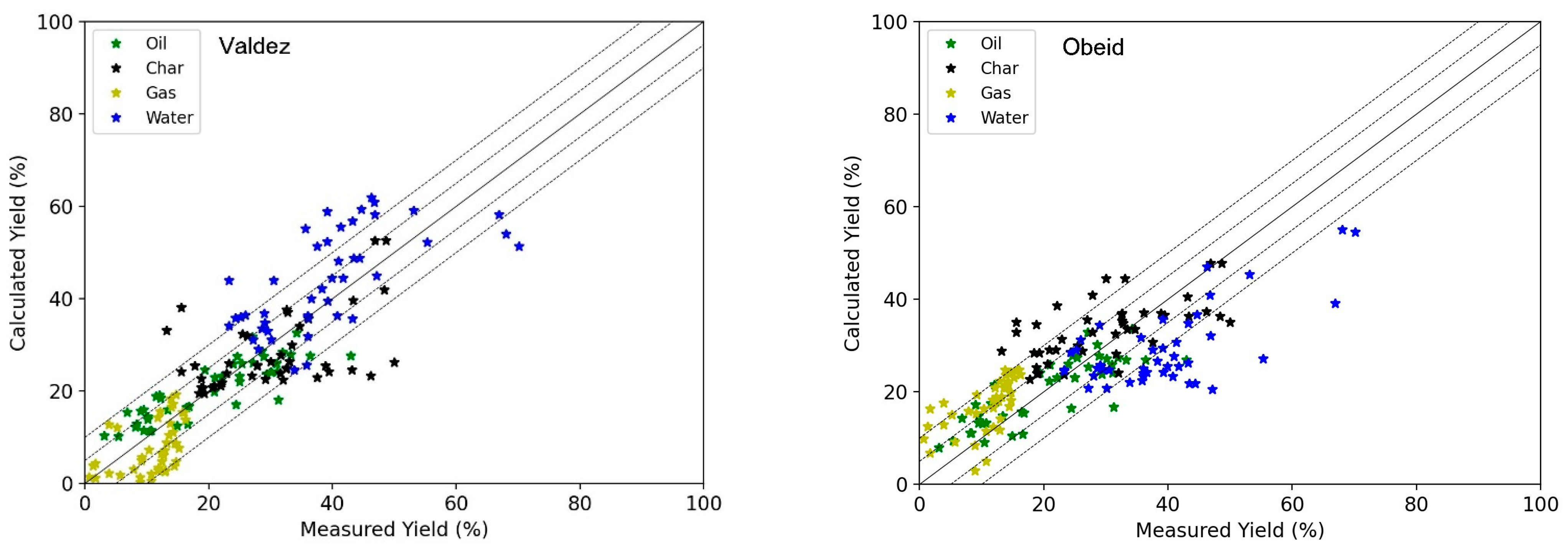
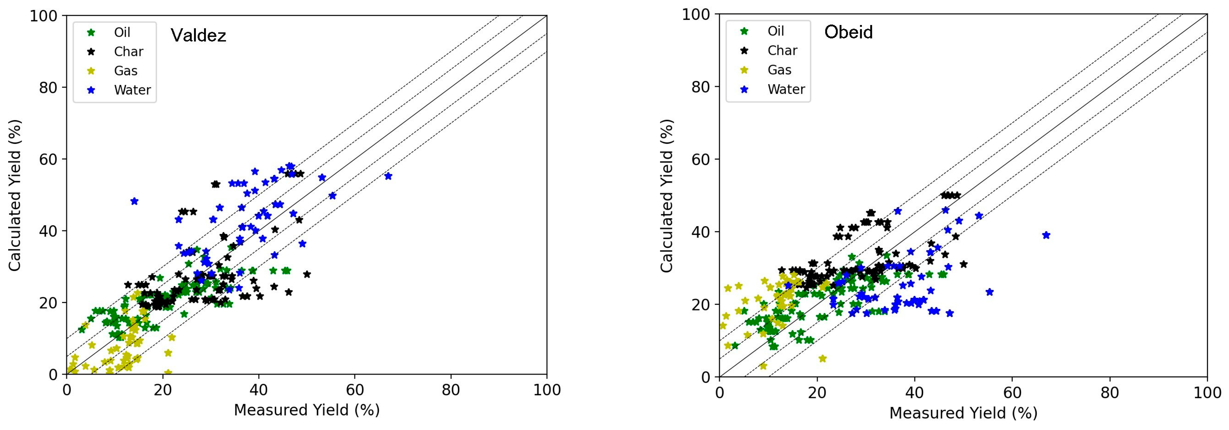
The reduced dataset consists of 44 lines in the data file, all with ethyl acetate as the extraction solvent. They consist of the resources described in detail in Section 2. Kinetic parameters for the models of Valdez and Obeid were determined through the optimisation procedure against this reduced dataset. Figure 4 below shows the results for the calculated yields with the optimised models of Valdez and Obeid on the experimental data for food wastes of the four different product phases: oil, char, gas, and organics in the aqueous phase (named water in the legends). Each of the phases is colour-coded, and this graph gives a visual representation of the fit result. Most points are centred around the parity line except for those of the aqueous phase (water) that are above or below, indicating a bad fit.

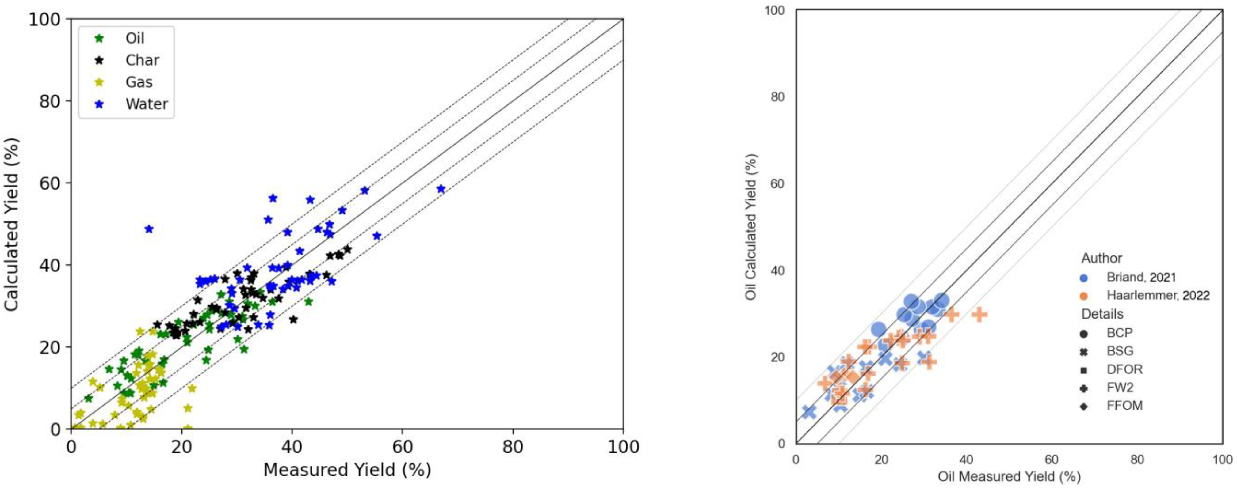
The results show, globally, a good prediction of the yields, except for the organics in aqueous phase that are not considered in the fitting of the model. The best results are for the oil yields prediction due to the higher weight given to the oil data. The results with the new model are presented in Figure 5. The model has a few more parameters, 19 reactions against 12 and 17 for Valdez and Obeid respectively. The better fit appears mainly due to the more complex reaction pathways that are possible with a model that is somewhat closer to reality.

The parity graphs give a relatively positive impression of the results, even for aqueous phase yields with calculated yields in the range of ± 10%.

Table 4. R² scores of the models trained with ethyl acetate data.

Model	Oil	Char	Gas	Aqueous Phase
Valdez	0.696	0.134	−0.886	0.135
Obeid	0.674	0.242	−2.053	−0.33
New Model	0.718	0.667	−0.895	0.092

compares the coefficient of determination, often referred to as the R² score, of the different models. A R² of one is a perfect fit, and zero or a negative value means that the model badly fits the model.

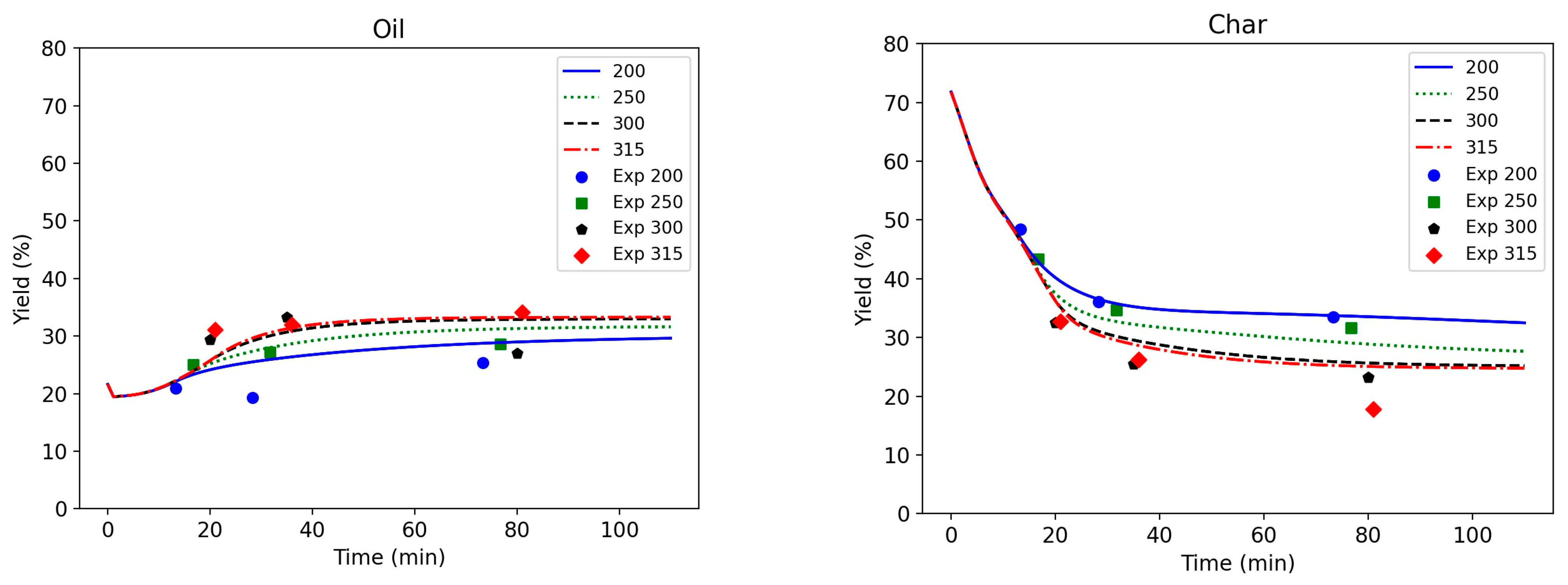
Figure 6 shows the evolution of the two most important products compared to the experimental data for blackcurrant pomace. There is quite some spread in the data, and the model also had to be composed with data from brewers’ spent grains and food waste, of quite a different nature.

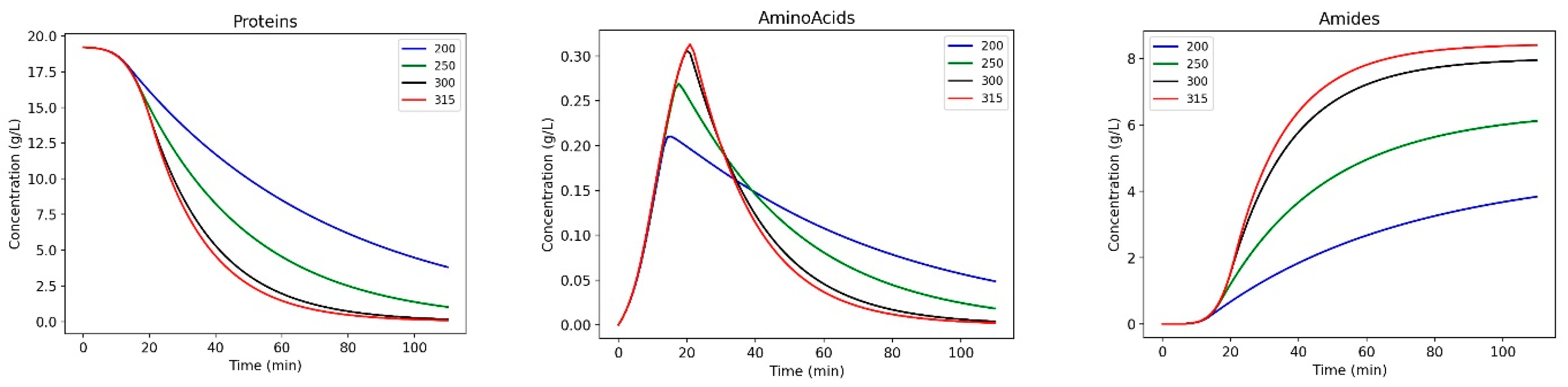
The char yield is decreasing as the initial dry matter is considered to be fully in the char product (as a solid phase). For a higher temperature, the final char yield is lower than the lowest temperature. For the oil yield, the trend is the other way around. Oil yields are higher at higher temperatures, and after 30 min, a kind of steady state is reached. The advantage of the new compositional model is that it allows for following the evolution of the different species in time. This helps to explain the form of the overall product graphs and to better understand the reactions. In Figure 7, it is shown that proteins are hydrolysed to form amino acids that, in turn, react with fatty acids to form amides. The model is able to capture the fact that hydrolysis is faster at higher temperatures, but it remains a rate-limiting step.

The kinetic parameters that make the models best fit the data are presented in

Table 5. Kinetic parameters in the models trained to the experimental data.

	Valdez		Obeid		New Model
	A	Ea	A	Ea	A	Ea
Units	mol−1 or L·g−1·mol−1	J·mol−1	mol−1 or L·g−1·mol−1	J·mol−1	mol−1 or L·g−1·mol−1	J·mol−1
Reaction0					9.421	16,407.6
Reaction1	0.152	13,046.4	0.065	23,019.81	9.922	17,400.21
Reaction2	0.685	1000.851	0.511	1010.577	11.438	6238.992
Reaction3	0.06	20,157.35	1.01	11,038.4	10.867	25,645.08
Reaction4	0.019	43,596.83	0.738	1000.23	10.68	18,720.6
Reaction5	0.195	14,919.05	0.125	17,386.63	9.696	20,541.66
Reaction6	0.512	6850.066	0.35	1001.63	9.606	8133.046
Reaction7	0.22	2054.016	0.082	20,907.09	10.068	15,063.84
Reaction8	0.116	46,329.72	0.268	7274.476	11.813	11,168.74
Reaction9	0.32	19,795.96	0.069	1000.88	12.084	27,161.62
Reaction10	0.00016	9419.418	0.401	8581.595	11.402	13,761.49
Reaction11	0.036	10,438.12	0.064	12,839.88	9.968	15,841.01
Reaction12	0.0045	502.059	0.449	16,834.57	2.139	18,122.33
Reaction13			0.09	38,058.25	13.732	10,000.03
Reaction14			0.00005	32,472.59	7.153	13,752.71
Reaction15			0.278	8949.258	11.194	18,520.29
Reaction16			0.06	1000.687	11.764	25,563.92
Reaction17			0.083	19,017.95	6.469	44,593.55
Reaction18					3.007	20,041.21

. The units for the pre-exponential factor depend on the order of the reaction as well as the number of reactants.

Sheehan and Savage [17] present kinetic data for the Valdez model on a data set for algae. They report pre-exponential factors in the range of 10⁻⁵ to 10⁻² (min⁻¹), slightly lower that the values presented in Table 5 for the same model. The activation energies they present are 50 to 140 kJ·mol⁻¹, and these values are higher than the values in Table 5. Sheehan and Savage report a R² for the oil yield of 0.45.

4.2. Fitting the Models to the Data Multiple Solvents

The models are now trained on a dataset containing more solvents. Many of the experiments were evaluated with different solvents. The dataset now consists of 96 experiments. This is a useful test, as it shows the ability of the models to adapt to different experimental protocols. Figure 8 below shows the results for the calculated yields with the optimised models of Valdez and Obeid on the experimental data.

The results show, globally, a good prediction of the yields, except for the organics in water phase that are not considered in the fitting of the model. The best results are for oil yields prediction due to the higher weight given to the oil data. The results with the new model are presented in Figure 9. Visually, the new model appears to be faring somewhat better. This should be of no surprise, as the compositional aspect allows for taking into account solvent characteristics, albeit in a simplified way.

The parity graphs, again, give a relatively positive impression of the results.

Table 6. R² score of the models trained with ethyl acetate data.

Model	Oil	Char	Gas	Aqueous Phase
Valdez	0.594	0.101	−2.042	−0.024
Obeid	0.564	0.173	−4.727	−1.313
New Model	0.680	0.647	−2.09	0.097

compares the coefficient of determination, often referred to as the R² score, of the different models. It shows that the new model significantly fares better that the Valdez and Obeid models.

Table 7. Kinetic parameters in the models trained to the experimental data produced with various solvents.

	Valdez		Obeid		New Model
	A	Ea	A	Ea	A	Ea
Units	mol−1 or L·g−1·mol−1	J·mol−1	mol−1 or L·g−1·mol−1	J·mol−1	mol−1 or L·g−1·mol−1	J·mol−1
Reaction0					7.21	18157.548
Reaction1	0.046	13,508.526	0.101	17,681.462	8.995	23,097.927
Reaction2	0.319	1000.017	0.399	1000.048	14.31	13,510.008
Reaction3	0.065	14,803.933	0.101	13,925.228	15.707	16,730.224
Reaction4	0.08	20,762.982	0.517	1000.627	12.52	18,696.677
Reaction5	0.089	13,260.351	0.108	15,819.529	12.02	20,237.533
Reaction6	0.454	7992.232	0.195	9098.875	13.797	7560.32
Reaction7	0.165	1001.746	0.091	18,184.555	11.944	15,612.032
Reaction8	0.158	22,380.493	0.201	7280.748	15.766	10,656.844
Reaction9	0.019	12,224.009	0.018	1001.517	9.632	21,999.27
Reaction10	0.0002	13,894.889	0.179	13,949.741	14.765	11,787.853
Reaction11	0.069	11,171.848	0.14	15,279.109	10.276	14,592.325
Reaction12	0.003	14,022.397	0.23	12,963.947	0.582	14,425.313
Reaction13			0.09	26,917.634	15.505	10,492.589
Reaction14			0.006	21,824.565	8.89	23,795.956
Reaction15			0.192	6298.809	13.584	29,343.481
Reaction16			0.108	4361.554	18.769	28,613.73
Reaction17			0.041	22,766.874	0.008	31,705.088
Reaction18					10.142	23,158.633

presents the kinetic parameters of the models trained with the extended data set taking into account different solvents. The values of the pre-exponential factors and activation energies are slightly different, but remain in the same order of magnitude for most reactions.

4.3. Extrapolating the Models to Literature Data

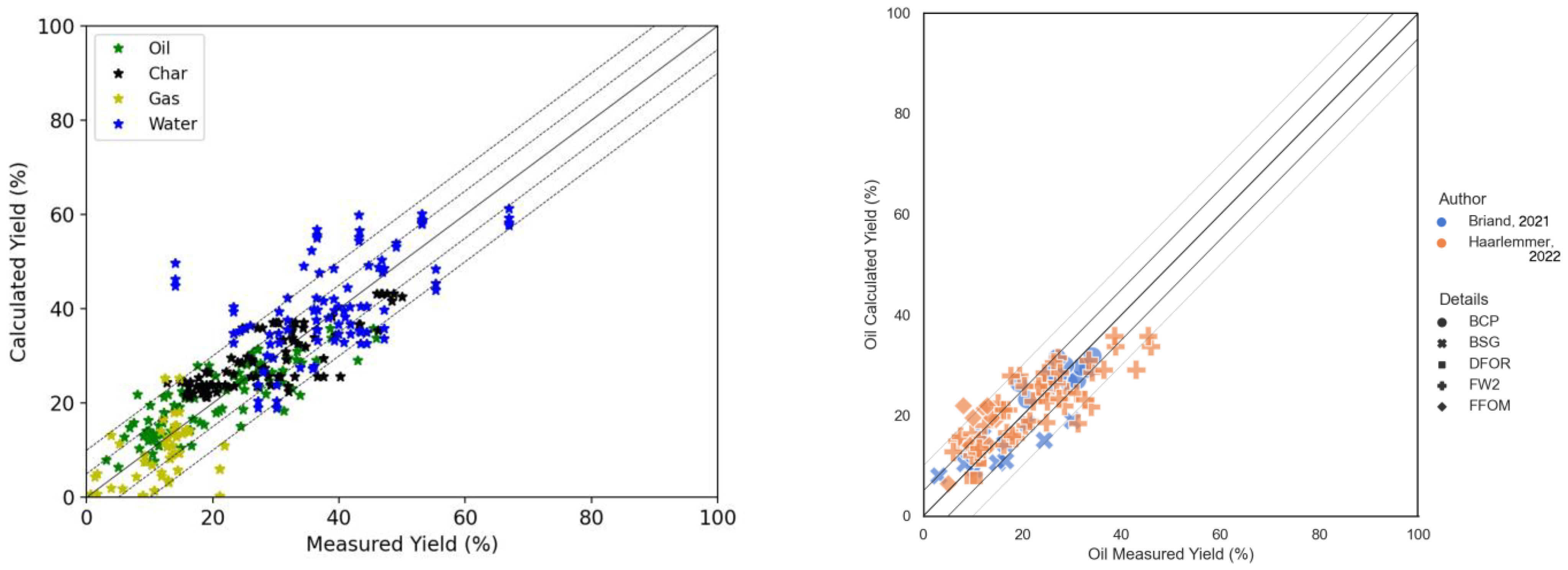
The trained models from Section 4.2 were applied to a large set of experimental data, including literature data, totalling 294 points. The models were trained exclusively on blackcurrant pomace, brewers’ spent grains, and food wastes collected from the CEA restaurant, including data with different solvents. This is the ultimate test for any model to show that it is universal. Figure 10 presents oil and char yields predicted with the new model.

The graphs show horizontally aligned points, often for a particular resource of a particular author. These points signify that the model gives the same result, even though the experimental data shows a certain dependency to process variables. The R² values are generally low.

Table 8. R² score of the models trained with ethyl acetate data.

Model	Oil	Char	Gas	Aqueous Phase
Valdez	0.664	−0.965	−0.131	−0.432
Obeid	0.686	−0.416	−1.913	−0.033
New Model	0.539	0.328	−1.861	−0.279

presents the result for the three models. Even though the new model performs less for the oil yields, it is slightly better on the char yield.

Even if there is a larger scattering of the results with some other experimental data, globally, all three models that were tested in this paper are able to reproduce results on a wide range of food wastes and agro-industrial wastes, processed at different HTL conditions and with different experimental ways of products recovery. The solvent effect is taken into account with an extremely simple model that can be improved.

Many explanations can be advanced to explain this inability to correctly represent the experimental results. Reactions are generally considered first order with the rate purely proportional to the concentration. The water concentration does not play a role. Considering that water takes part in the reactions, some deviation of a first order is to be expected. In an earlier paper on the same dataset [6], it was shown that even with very advanced regression tools, some spread in the results cannot be avoided. The data is typically regrouped around the parity line, with most of the data with a 10% deviation. This natural spread should be imputed to differences in the limited descriptions of the experimental practices and experimental uncertainty, but also in resource characterisation. Considering that clusters of outliers are often associated with one author suggests that there may be systematic differences. These differences potentially include resource analysis techniques. A wide variety of analysis techniques are used in the literature to estimate carbohydrate, lipid, and protein content. Each of these techniques produce their own estimate of the composition.

Simplified models dealing only with final products do not allow to really understand the chemistry. In the Valdez model, there is no char product and the unconverted resources are counted as char, obliging the model to limit the conversion of the resource to allow for some char. These models are better suited for algae or other resources producing little char. However, even with this limitation, this model gives good results. A perfect fit is not possible, as previously published studies with machine learning algorithms have shown that there is a minimal incompressible dispersion that cannot be avoided.

5. Conclusions

The kinetic models presented in the literature are generally trained to a limited set of experimental data, showing generally good results. The models presented in this paper have shown that they can be trained on a limited experimental dataset and then applied to a much wider set of data. As the models have a sufficient number of kinetic parameters, reasonably good results can be obtained.

The advantage of a compositional model is that it allows for following the evolution of the different species in time. This type of model can be trained on a particular resource and applied on another. It also allows for the adaptation of the model to different extraction techniques and solvents, extending the application field of a trained model.

The next steps are to quantify intermediate and final product families of compounds and include these in the model training to obtain a better validation of the conversion routes and more accurate prediction results in term of global oil and char yields, but also molecular composition of those product phases.