
Use of Continuous Wavelet Transform to Generate Endurance Time Excitation Functions for Nonlinear Seismic Analysis of Structures
Abstract
:1. Introduction
- -
- Investigate various real earthquakes via continuous wavelet transform in the time-frequency domain.
- -
- Extract important ground motion characteristics from these earthquakes for use in generating new endurance time excitation functions (ETEFs).
- -
- Generate ETEFs with ground motion characteristics that match the geometric mean response spectrum of these real earthquakes.
- -
- Perform endurance time analyses on steel and reinforced concrete structures using these ETEFs and compare the results with those obtained from an incremental dynamic analysis (IDA), which is considered to be the most sophisticated method of analysis; or the time history analysis (THA) using multiple earthquakes.
2. Endurance Time Analysis (ETA) Method
3. Wavelet Transform and Wavelet Analysis
3.1. Wavelet Coefficients
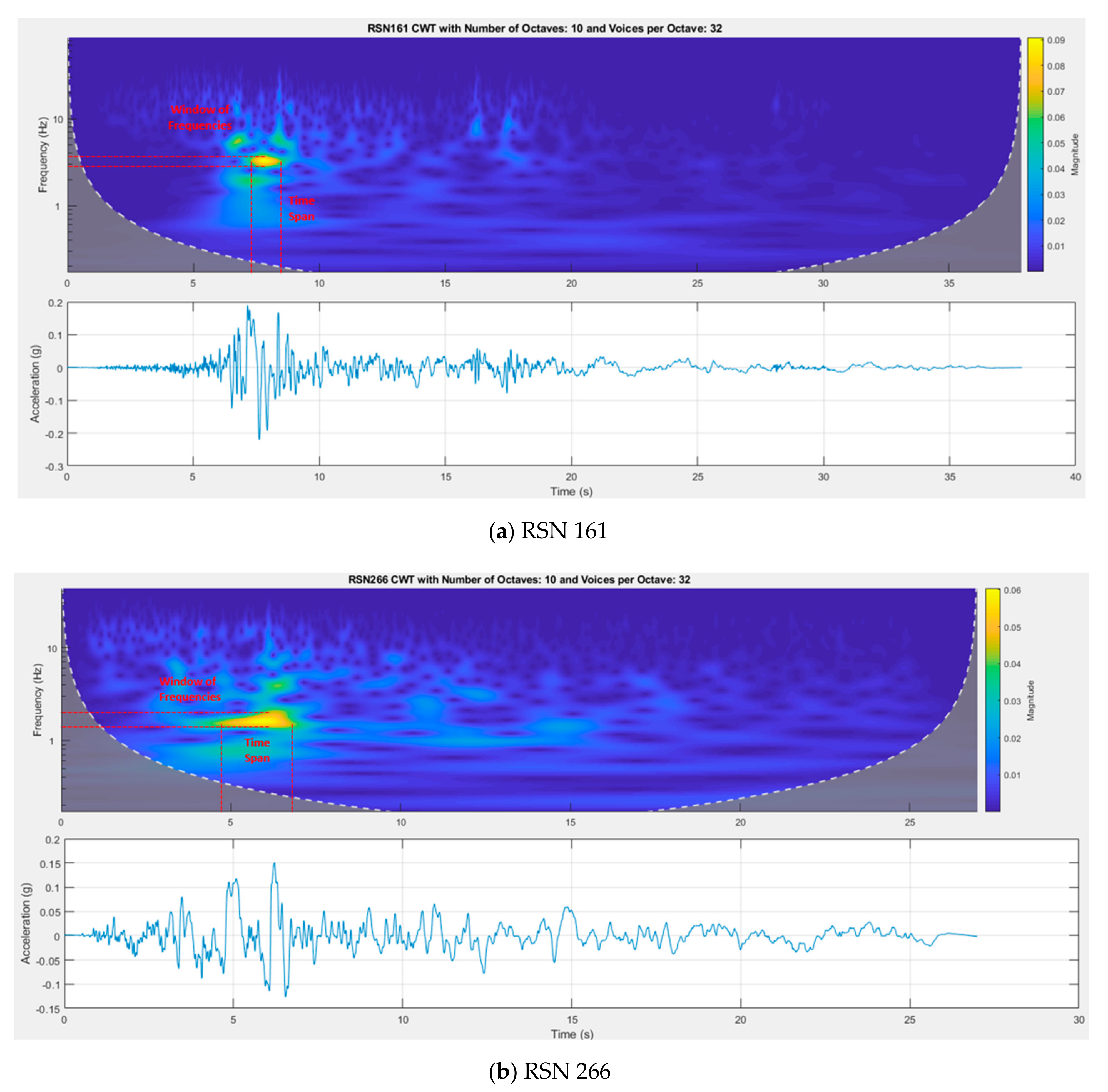
3.2. Wavelet Map
3.3. Morse Wavelets
4. Generation of Artificial Ground Motions and ETEFs
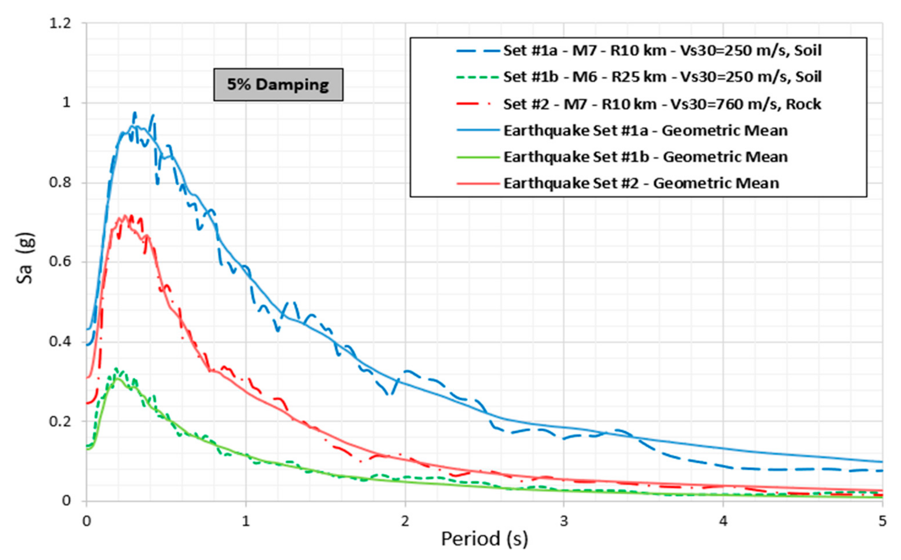
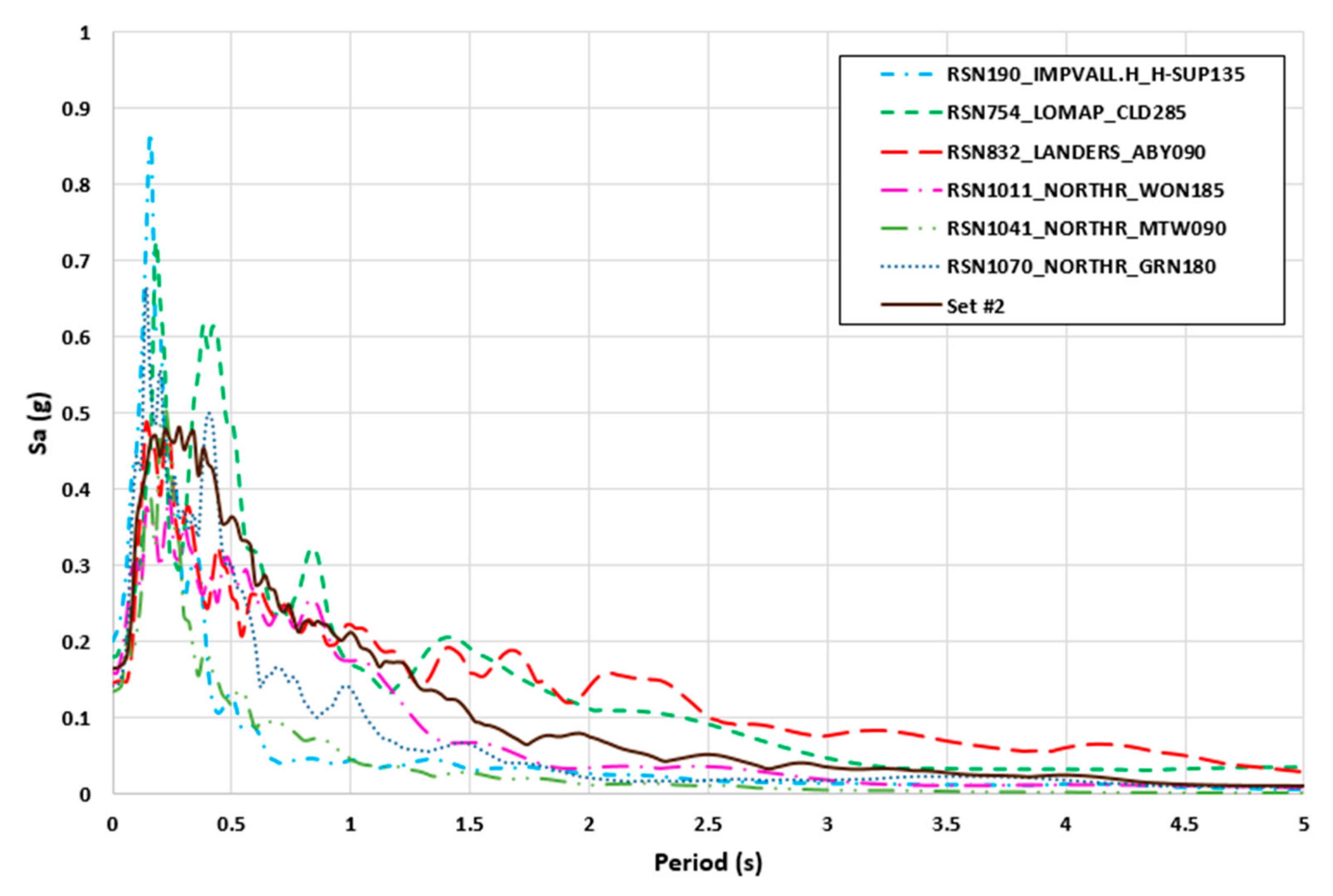
4.1. Ground Motion Data
4.2. Wavelet Maps
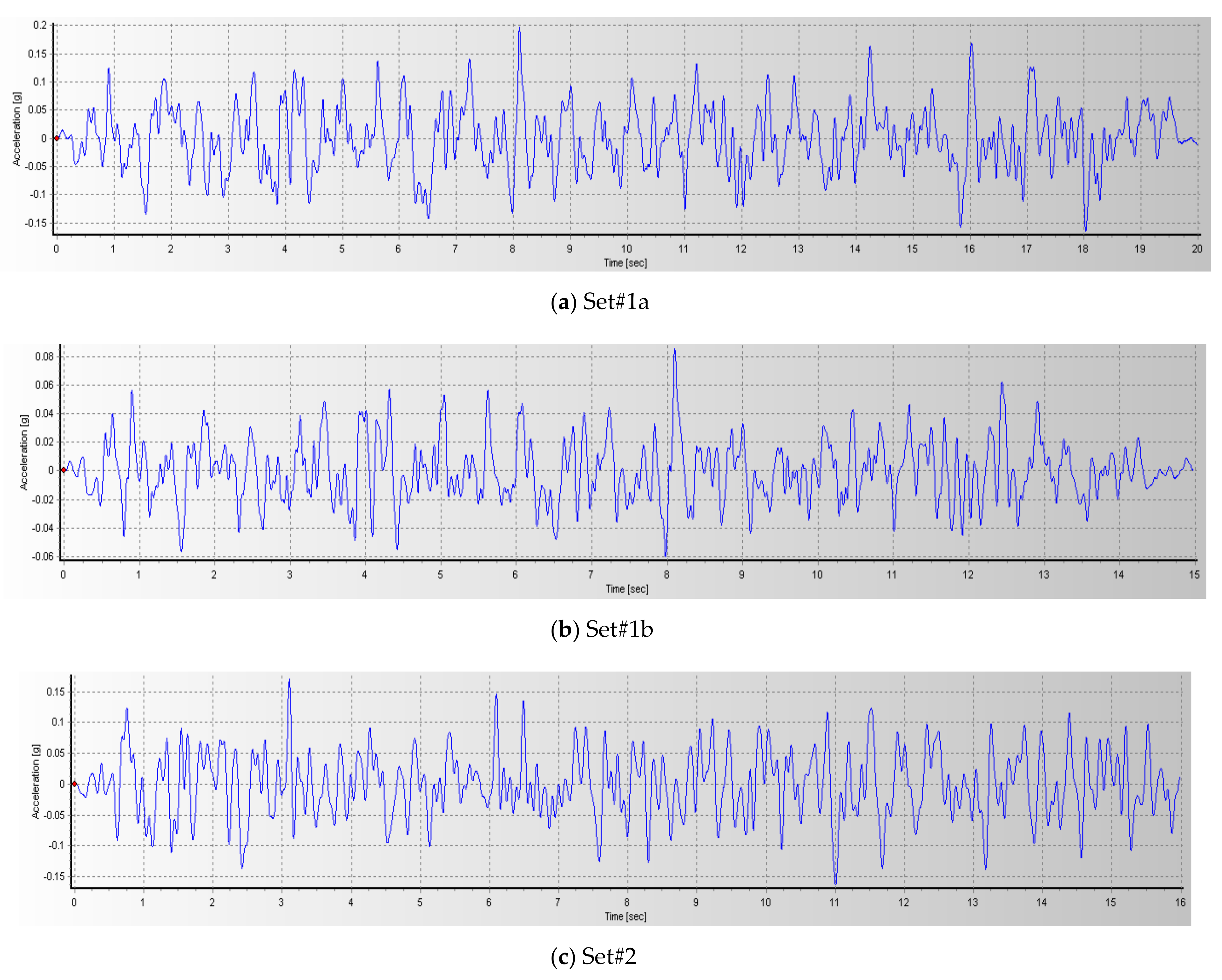
4.3. Generation of Artificial Excitations
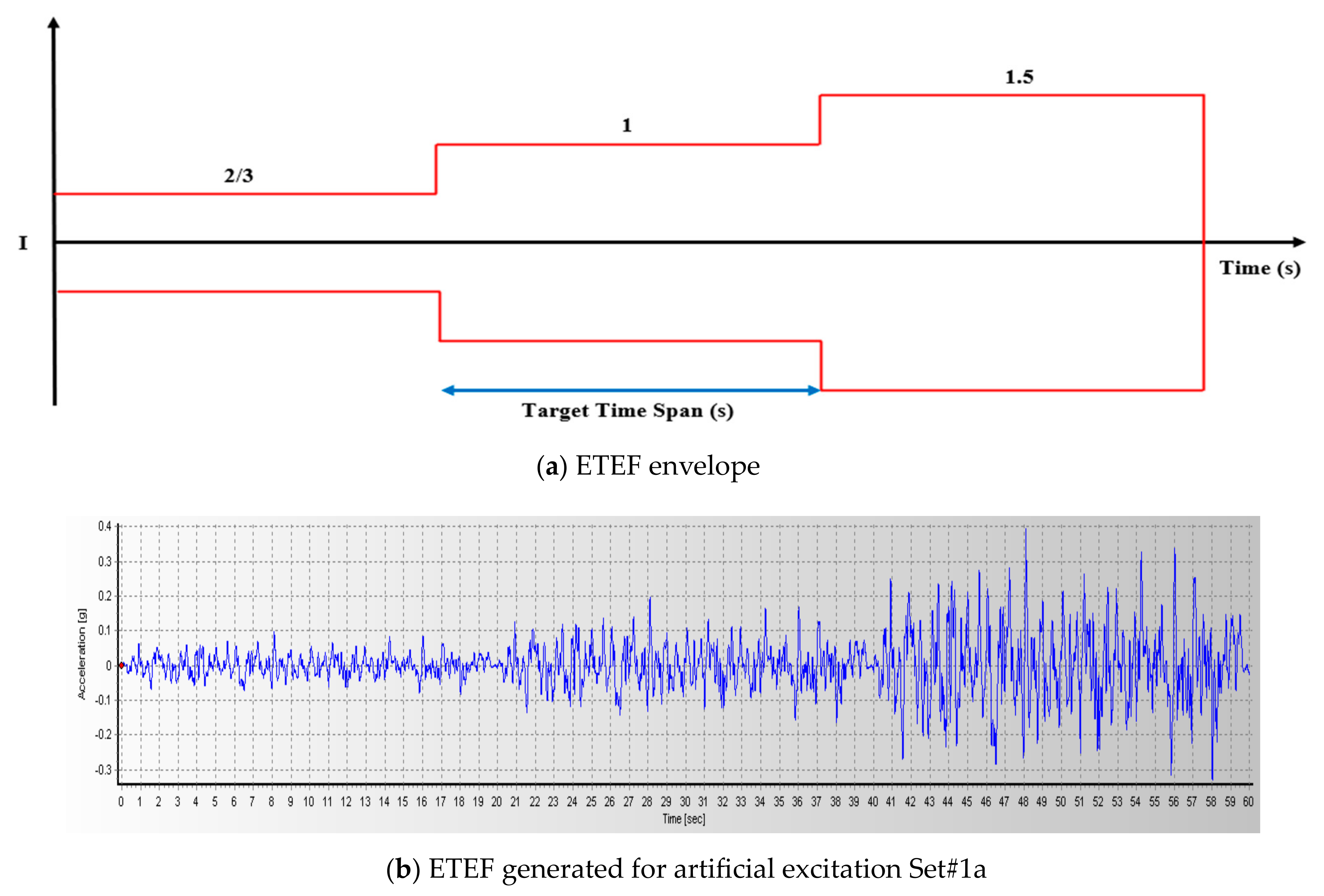
4.4. Generation of Intensifying ETEFs
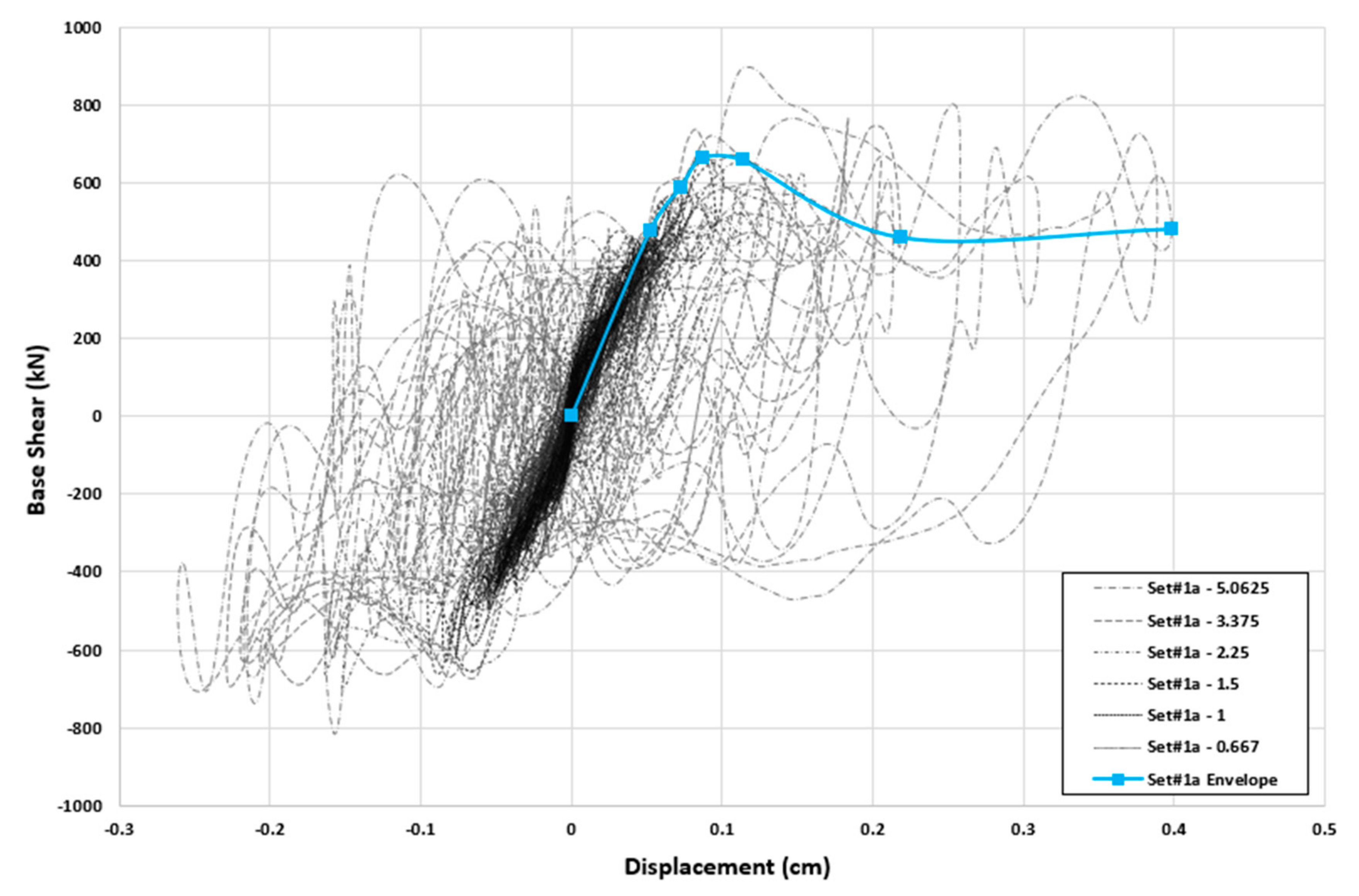
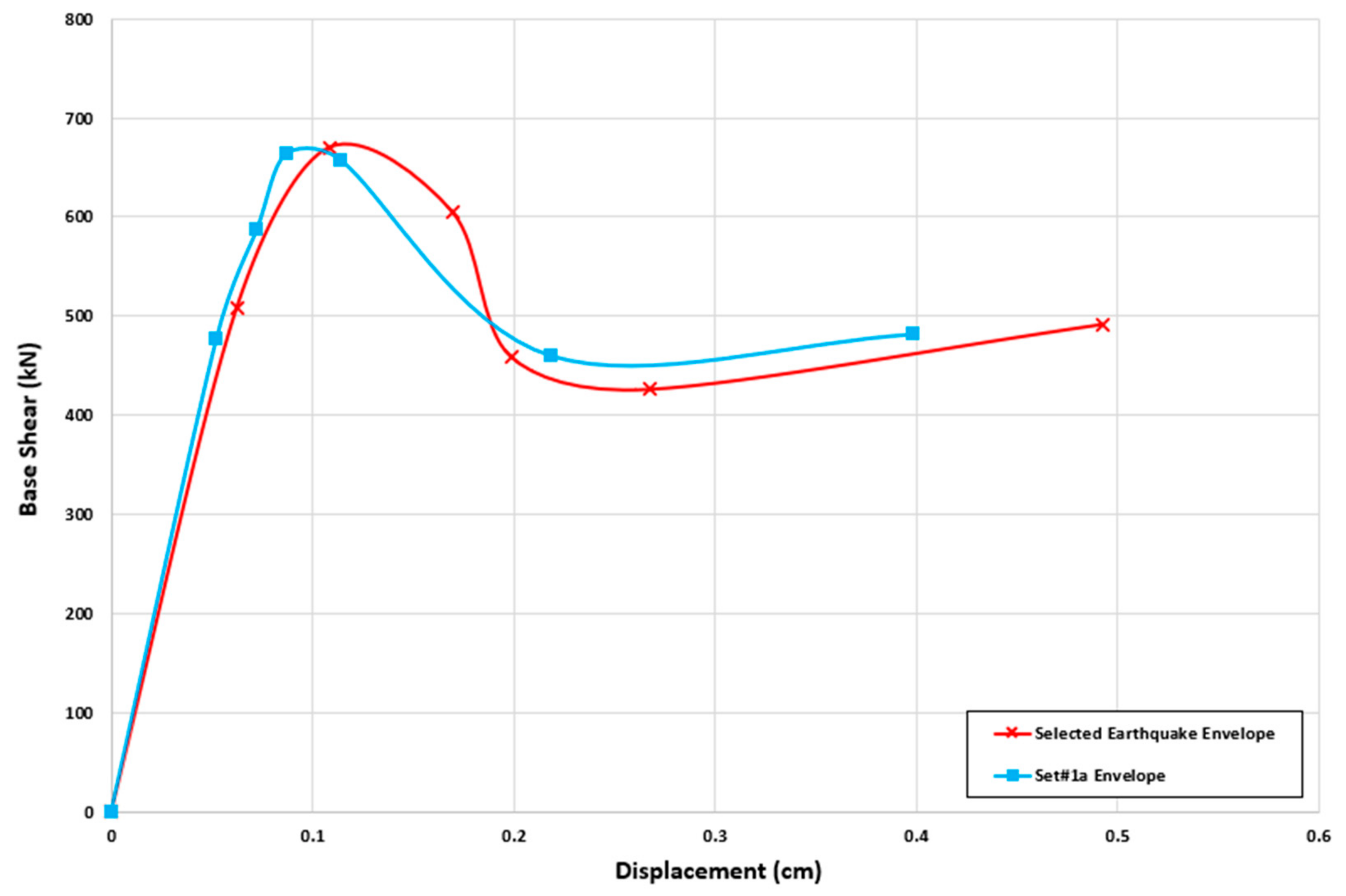
5. Application of ETA to Steel and Concrete Structures
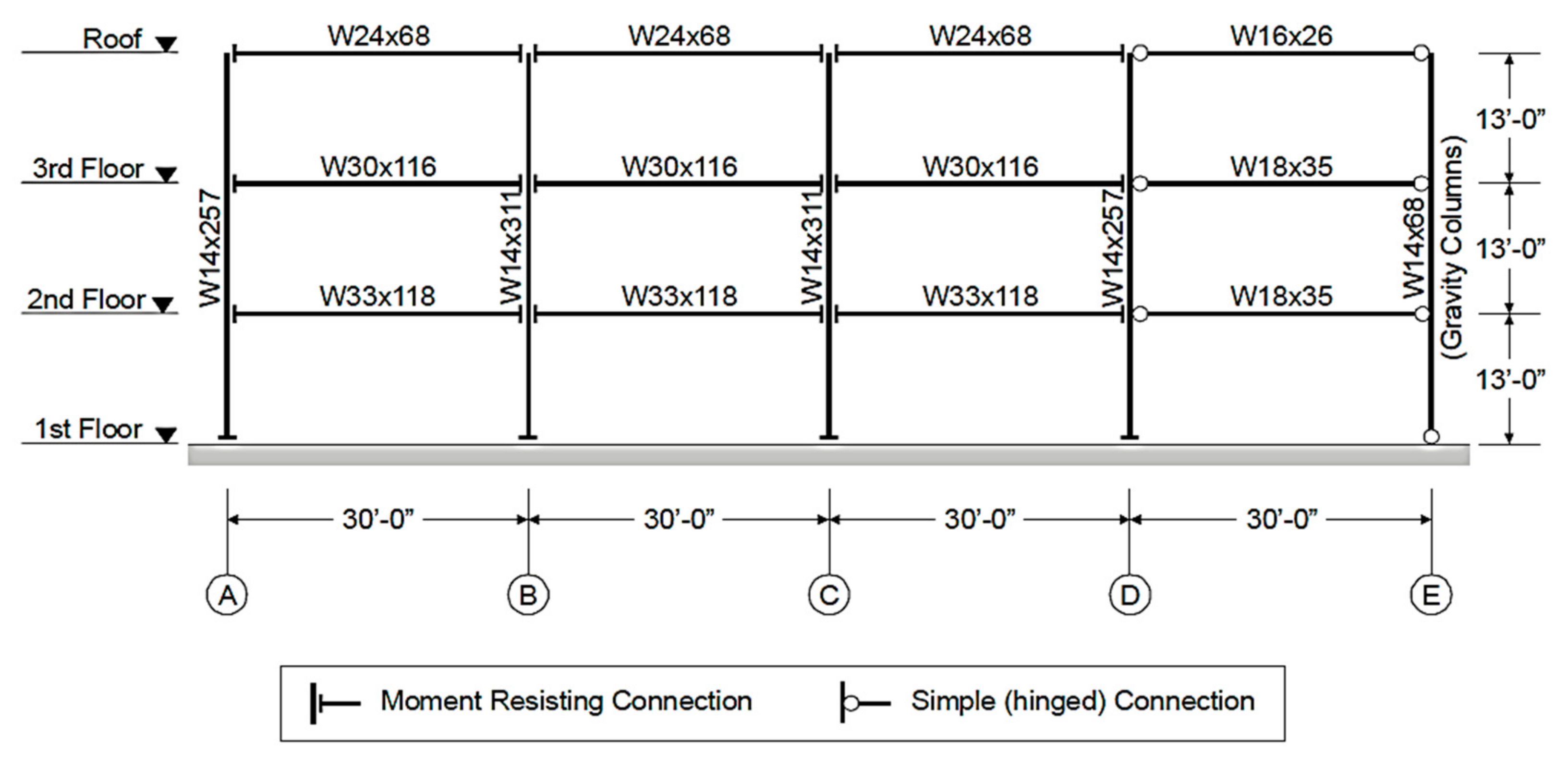
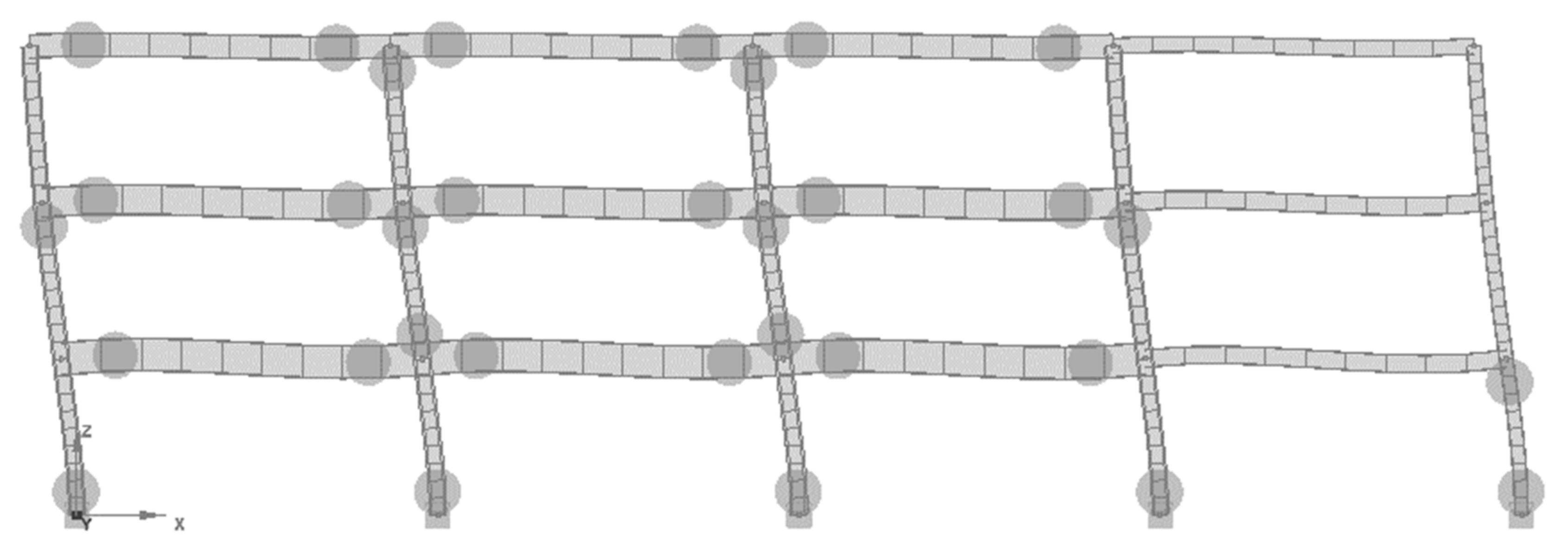
5.1. FEMA 440 Benchmark Steel Frame Structure
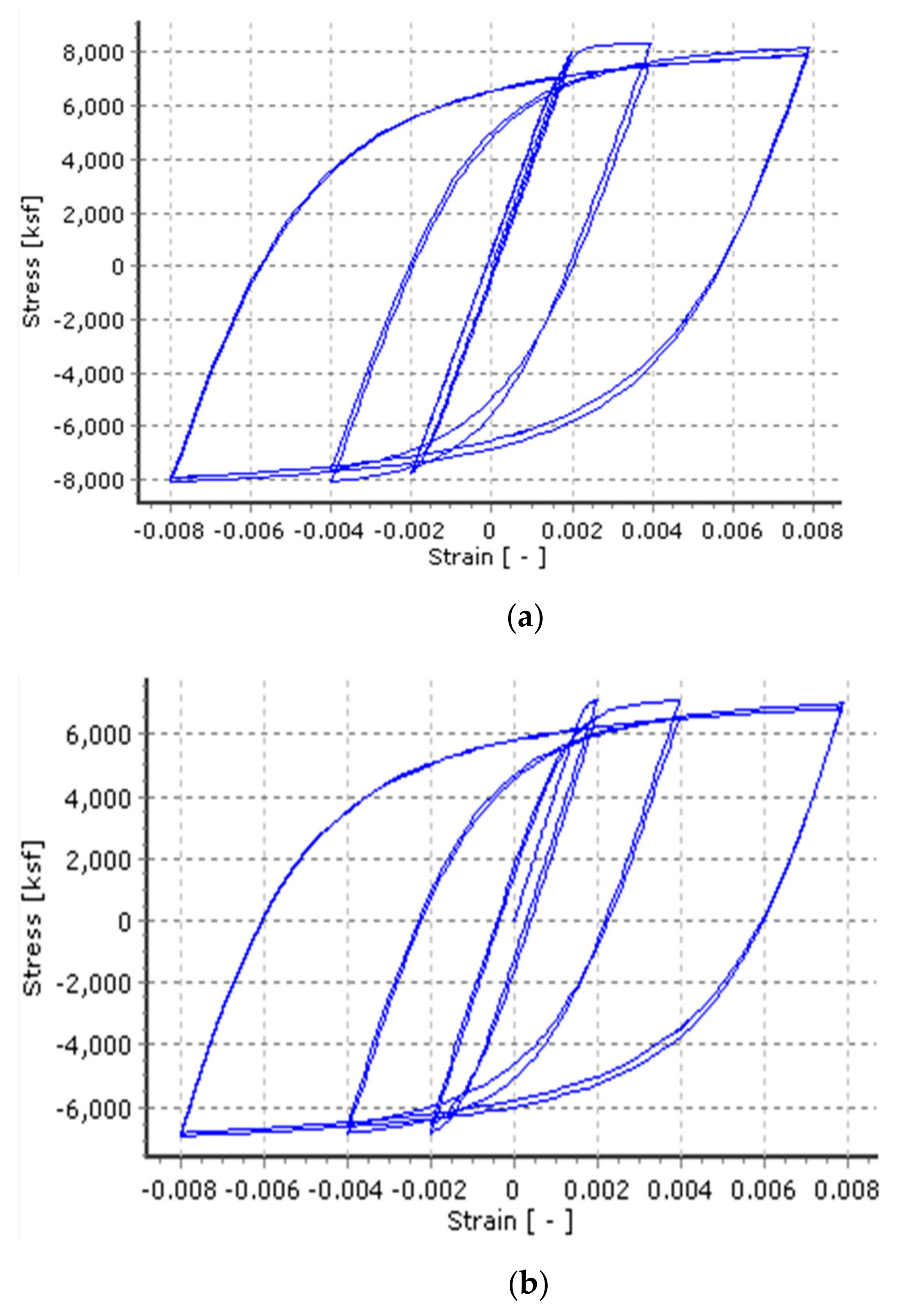
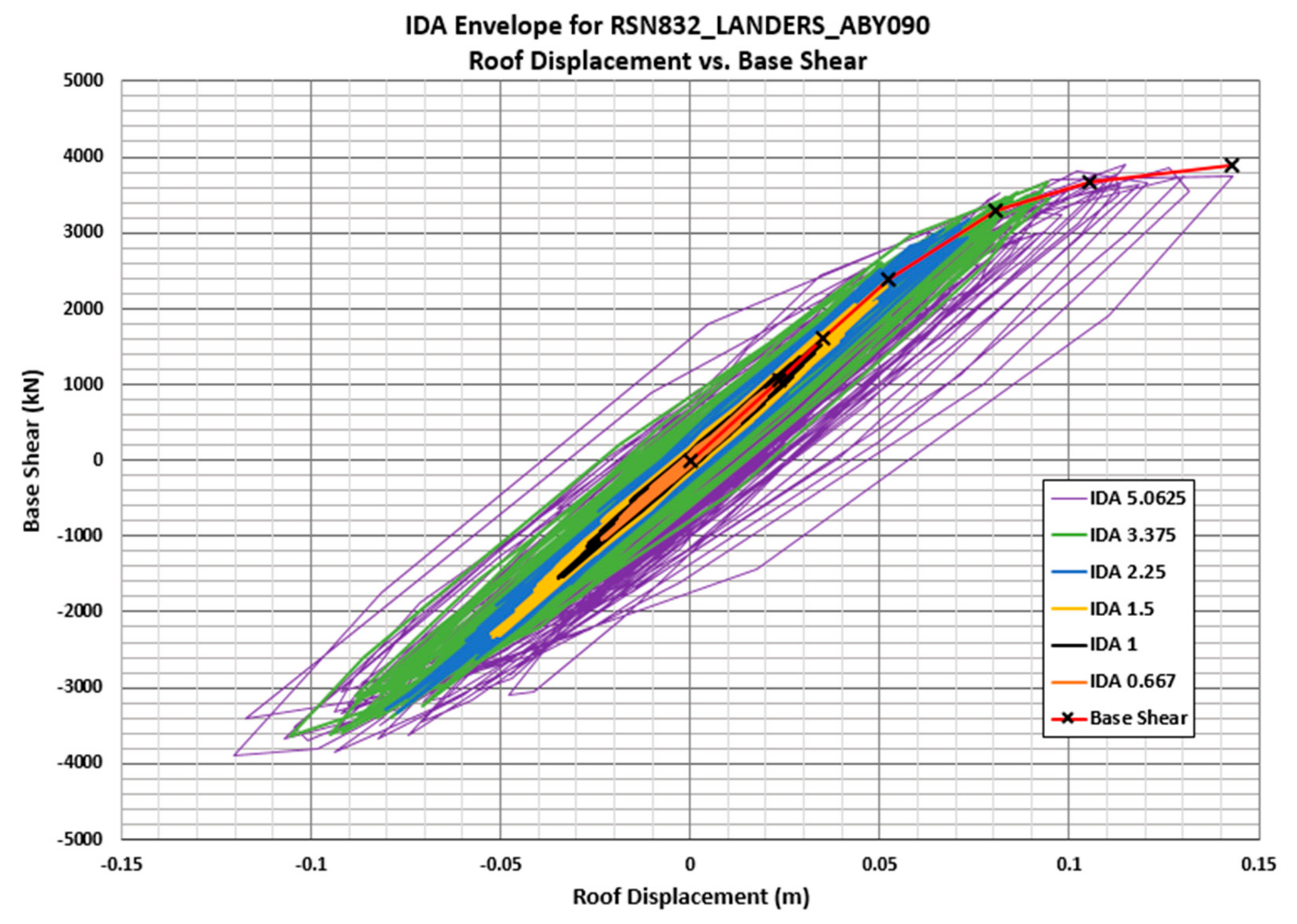
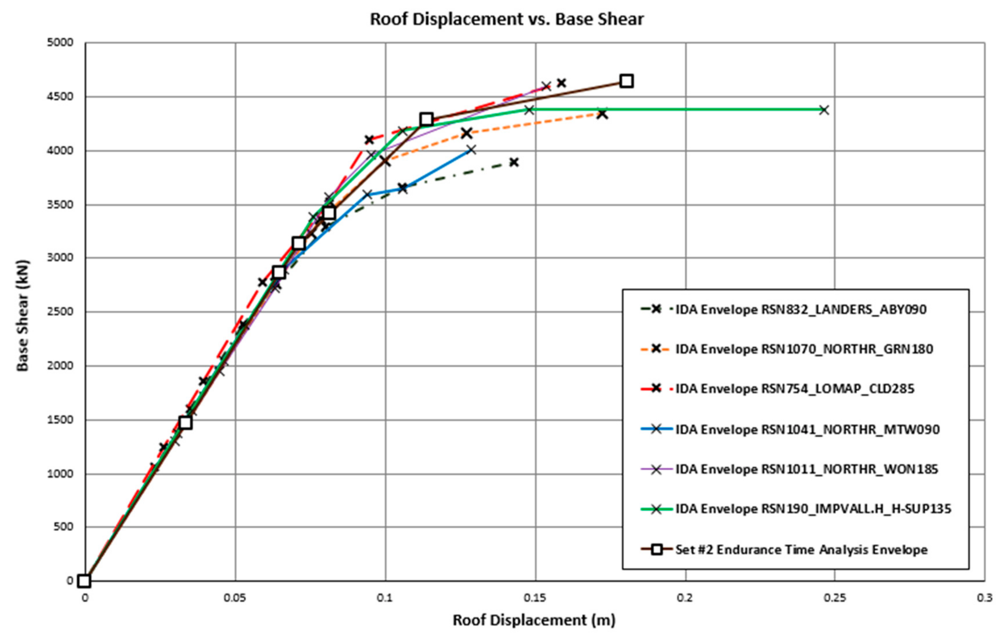
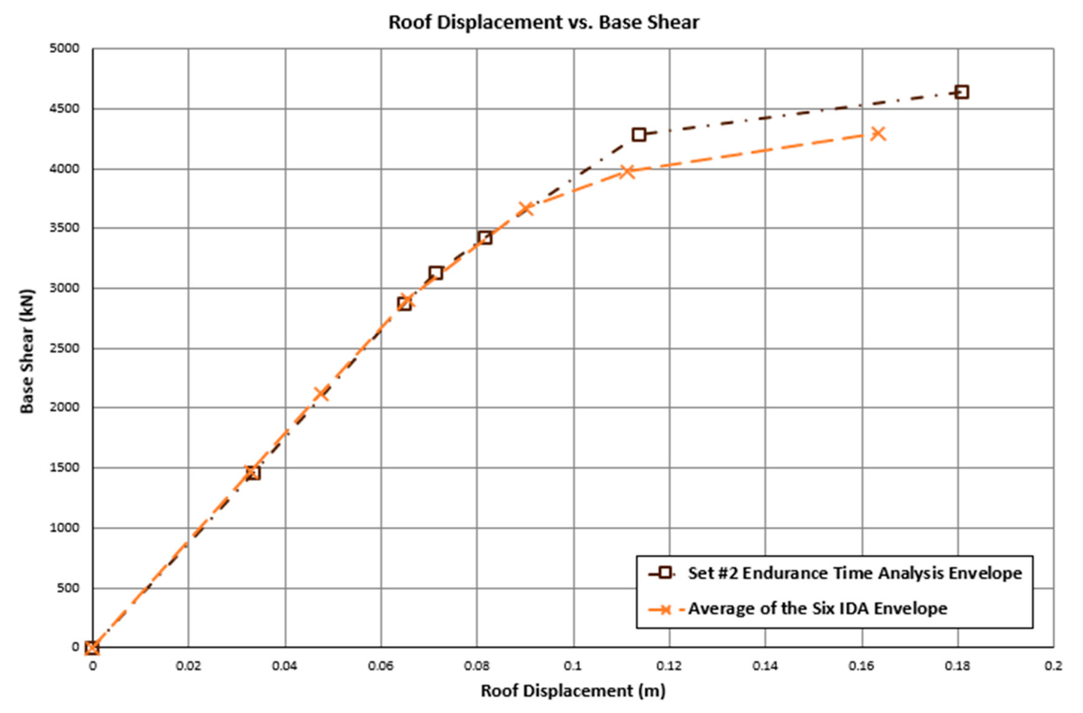
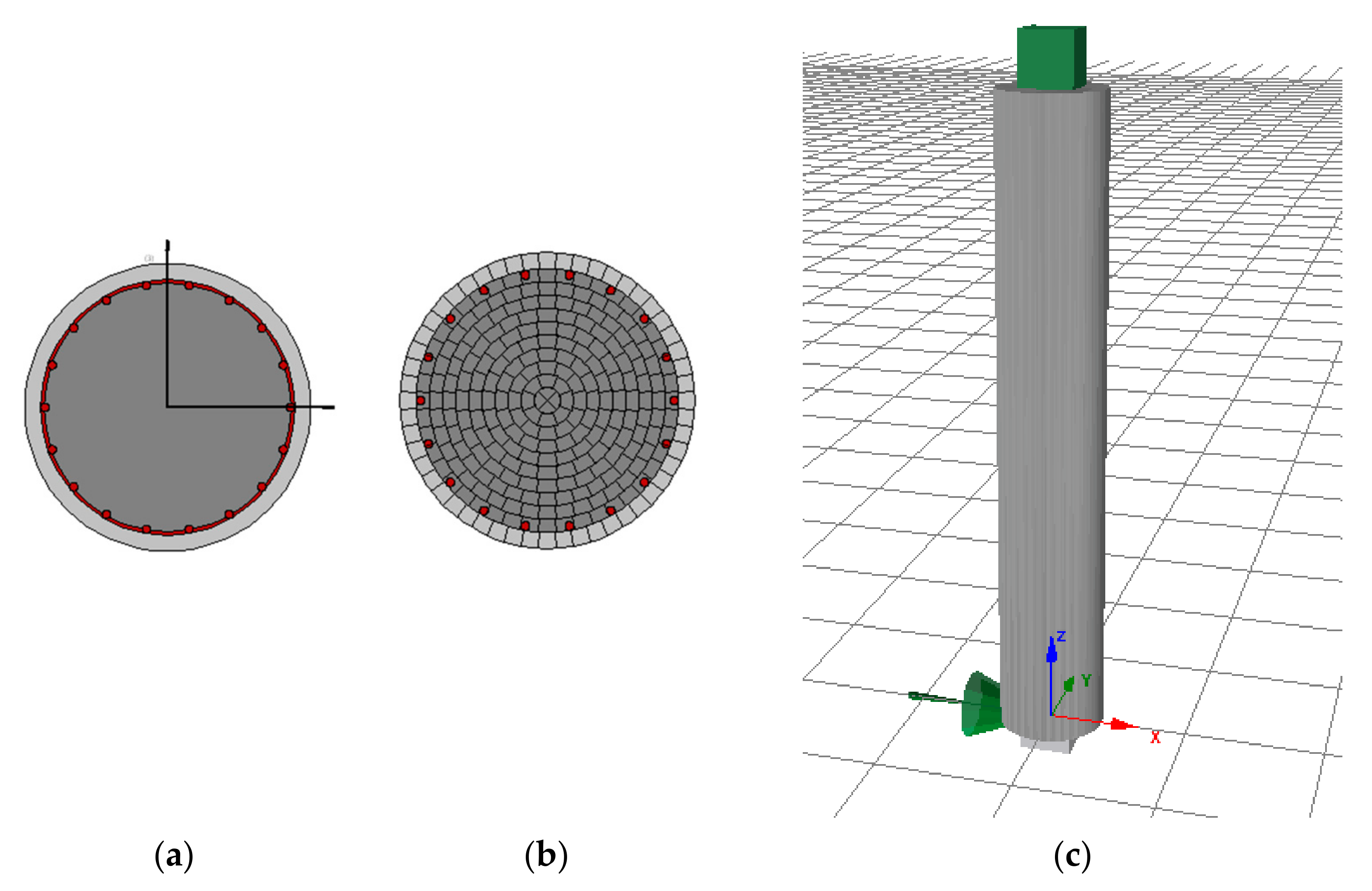
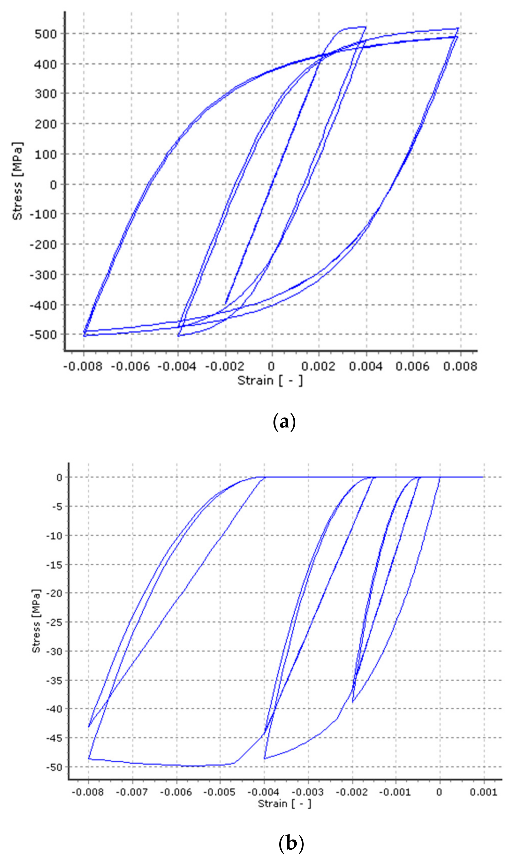
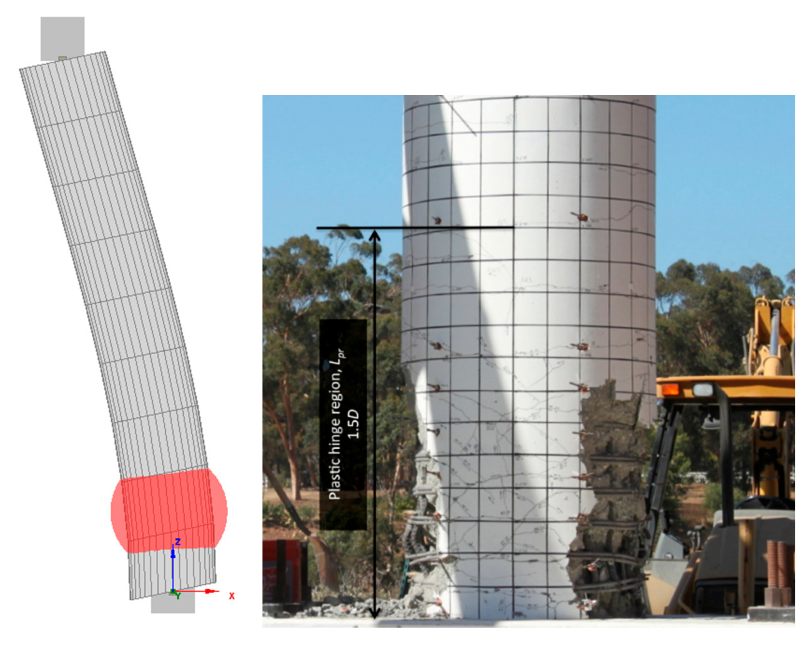
5.2. Single-Column Bridge Bent
6. Summary
- (1)
- Select ground motions that are representative of the site conditions.
- (2)
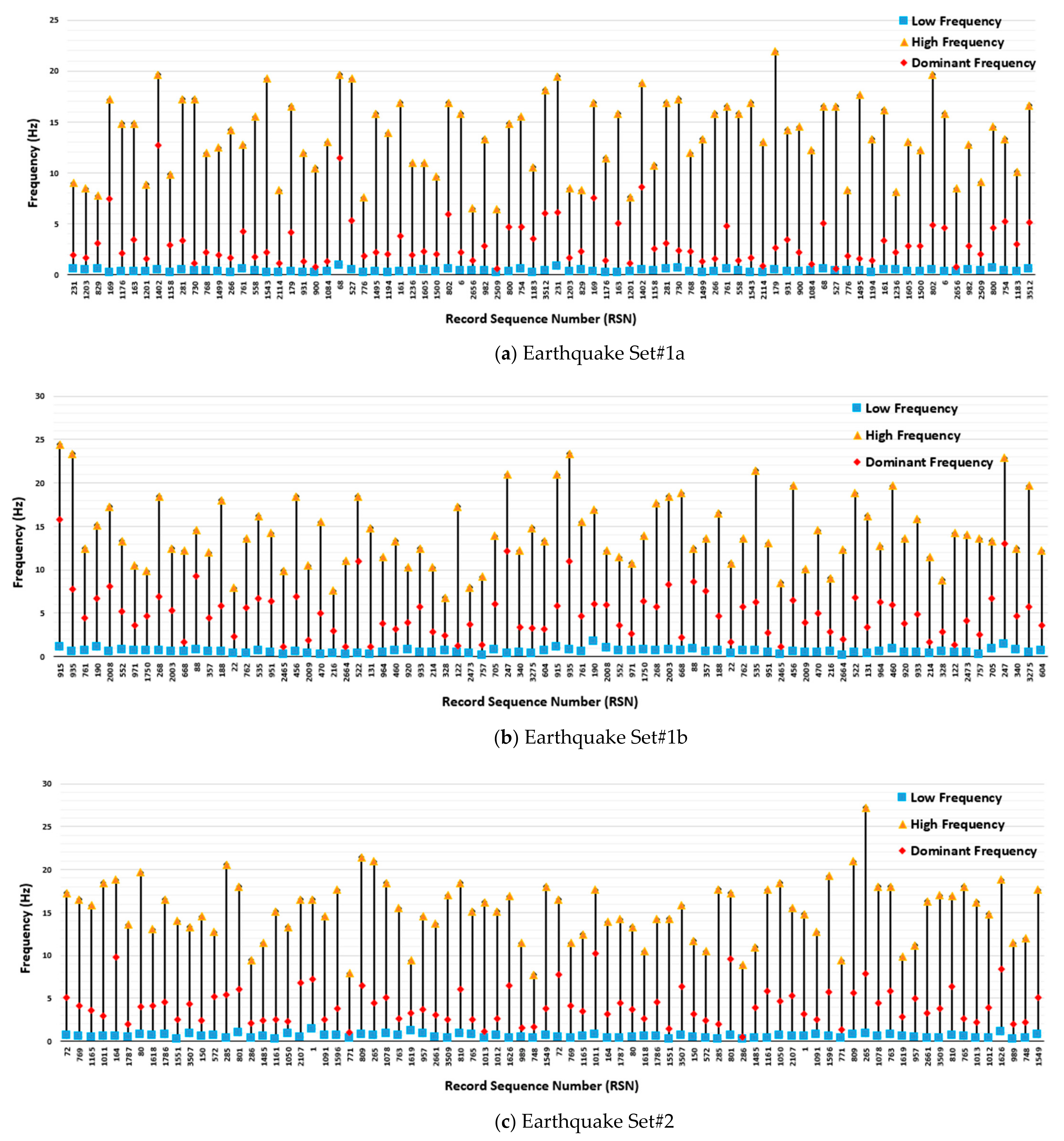
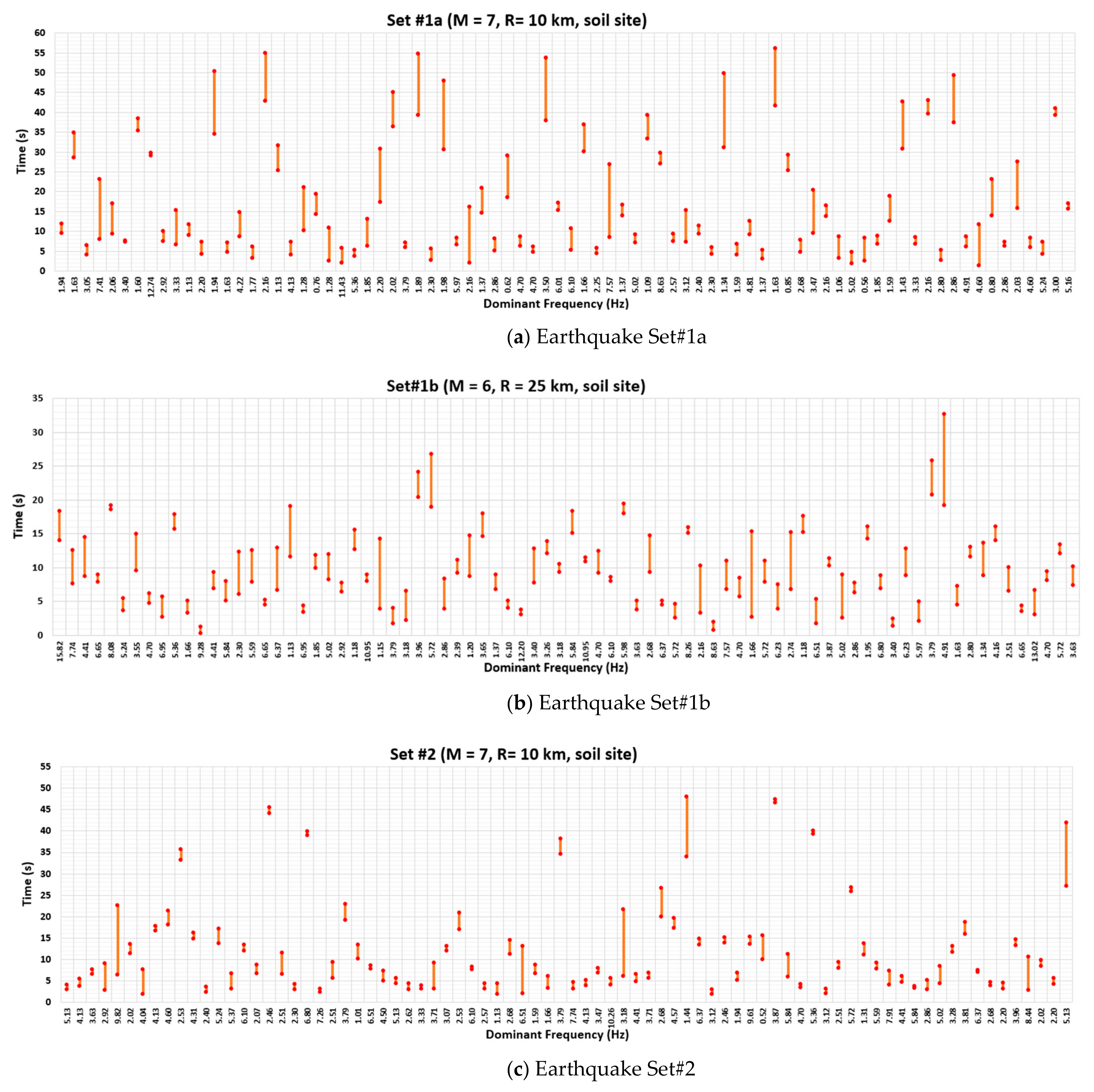
- Perform wavelet analysis on these ground motions to identify their frequency contents, the dominant frequencies, windows of frequencies (frequencies that are within 10% of the dominant frequencies) and the corresponding time durations.
- (3)
- Perform statistical analysis to determine the frequency range that contains at least 90% of the frequency contents of these ground motions and to identify the 90 percentile time duration for the windows of the frequencies.
- (4)
- Generate artificial excitation with a time duration equal to that obtained in Step 3 using the geometric mean of the selected set of ground motions as the target response spectrum.
- (5)
- Correct the frequency contents of the artificial earthquake generated in Step 4 based on data obtained in Step 3 using the sixth-order Type 1 Chebyshev filter function.
- (6)
- Regenerate the artificial excitation and intensify it using a block-shaped intensifying envelope.
Supplementary Materials
Author Contributions
Funding
Data Availability Statement
Acknowledgments
Conflicts of Interest
Appendix A. Earthquake Data Set (Adapted from Baker et al. [49])

| Earthquake Set#1a | Earthquake Set#1b | Earthquake Set#2 | ||||||
|---|---|---|---|---|---|---|---|---|
| RSN | Earthquake (Station) | M | RSN | Earthquake (Station) | M | RSN | Earthquake (Station) | M |
| 231 | Mammoth Lakes-01 (Long Valley Dam, Upr L Abut) | 6.1 | 915 | Big Bear-01 (Lake Cachulla) | 6.5 | 72 | San Fernando (Lake Hughes #4) | 6.6 |
| 1203 | Chi-Chi, Taiwan (CHY036) | 7.6 | 935 | Big Bear-01 (Snow Creek) | 6.5 | 769 | Loma Prieta (Gilroy Array #6) | 6.9 |
| 829 | Cape Mendocino (Rio Dell Overpass—FF) | 7.0 | 761 | Loma Prieta (Fremont, Emerson Court) | 6.9 | 1165 | Kocaeli, Turkey (Izmit) | 7.5 |
| 169 | Imperial Valley-06 (Delta) | 6.5 | 190 | Imperial Valley-06 (Superstition Mtn Camera) | 6.5 | 1011 | Northridge-01 (LA-Wonderland Ave. | 6.7 |
| 1176 | Kocaeli, Turkey (Yarimca) | 7.5 | 2008 | CA/Baja Border Area (El Centro Array #7) | 5.3 | 164 | Imperial Valley-06 (Cerro Prieto) | 6.5 |
| 163 | Imperial Valley-06 (Calipatria Fire Sta.) | 6.5 | 552 | Chalfant Valley-02 (Lake Crowley, Sherhorn Res.) | 6.2 | 1787 | Hector Mine (Hector) | 7.1 |
| 1201 | Chi-Chi, Taiwan (CHY034) | 7.6 | 971 | Northridge-01 (Elizabeth Lake) | 6.7 | 80 | San Fernando (Pasadena-Old Seis. Lab.) | 6.6 |
| 1402 | Chi-Chi, Taiwan (NST) | 7.6 | 1750 | Northwest China-02 (Jiashi) | 5.9 | 1618 | Duzce, Turkey (Lamont 531) | 7.1 |
| 1158 | Kocaeli, Turkey (Duzce) | 7.5 | 268 | Victoria, Mexico (SAHOP Casa Flores) | 6.3 | 1786 | Hector Mine (Heart Bar State Park) | 7.1 |
| 281 | Trinidad (Rio Dell Overpass, E Ground) | 7.2 | 2003 | CA/Baja Border Area (Calexico Fire Station) | 5.3 | 1551 | Chi-Chi, Taiwan (TCU138) | 7.6 |
| 730 | Spitak, Armenia (Gukasian) | 6.8 | 668 | Whittier Narrows-01 (Norwalk, Imp Hwy S Grnd) | 6.0 | 3507 | Chi-Chi, Taiwan (TCU129) | 6.3 |
| 768 | Loma Prieta (Gilroy Array #4) | 6.9 | 88 | San Fernando (Santa Felita Dam Outlet) | 6.6 | 150 | Coyote Lake (Gilroy Array #6) | 5.7 |
| 1499 | Chi-Chi, Taiwan (TCU060) | 7.6 | 357 | Coalinga-01 (Parkfield, Stone Corral 3E) | 6.4 | 572 | Taiwan SMART1(45) (SMART1 E02) | 7.3 |
| 266 | Victoria, Mexico (Chihuahua) | 6.3 | 188 | Imperial Valley-06 (Plastic City) | 6.5 | 285 | Irpinia, Italy-01 (Bagnoli Irpinio) | 6.9 |
| 761 | Loma Prieta (Fremont—Emerson Ct.) | 6.9 | 22 | El Alamo (El Centro Array #9) | 6.8 | 801 | Loma Prieta (San Jose-Santa Teresa Hills) | 6.9 |
| 558 | Chalfant Valley-02 (Zack Brothers Ranch) | 6.2 | 762 | Loma Prieta (Fremont, Mission San Jose) | 6.9 | 286 | Irpinia, Italy-01 (Bisaccia) | 6.9 |
| 1543 | Chi-Chi, Taiwan (TCU118) | 7.6 | 535 | N. Palm Springs (San Jacinto, Valley Cementary) | 6.1 | 1485 | Chi-Chi, Taiwan (TCU045) | 7.6 |
| 2114 | Denali, Alaska (TAPS Pump Sta. #10) | 7.9 | 951 | Northridge-01 (Bell Gardens, Jaboneria) | 6.7 | 1161 | Kocaeli, Turkey (Gebze) | 7.5 |
| 179 | Imperial Valley-06 (El Centro Array #4) | 6.5 | 2465 | Chi Chi, Taiwan (CHY034) | 6.2 | 1050 | Northridge-01 (Pacoima Dam, downstr) | 6.7 |
| 931 | Big Bear-01 (San Bernardino, E and Hospitality) | 6.5 | 456 | Morgan Hill (Gilroy Array #2) | 6.2 | 2107 | Denali, Alaska (Carlo, temp) | 7.9 |
| 900 | Landers (Yermo Fire Sta.) | 7.3 | 2009 | CA/Baja Border Area (Holtville Post Office) | 5.3 | 1 | Helena, Montana-01 (Carroll College) | 6.0 |
| 1084 | Northridge-01 (Sylmar—Converter Station) | 6.7 | 470 | Morgan Hill (San Juan Bautista, 24 Polk St.) | 6.2 | 1091 | Northridge-01 (Vasquez Rocks Park) | 6.7 |
| 68 | San Fernando (LA-Hollywood Stor FF) | 6.6 | 216 | Livermore-01 (Tracy, Sewage Treatment Plant) | 5.8 | 1596 | Chi-Chi, Taiwan (WNT) | 7.6 |
| 527 | N. Palm Springs (Morongo Valley) | 6.1 | 2664 | Chi-Chi, Taiwan-03 (TCU145) | 6.2 | 771 | Loma Prieta (Golden Gate Bridge) | 6.9 |
| 776 | Loma Prieta (Hollister—South and Pine) | 6.9 | 522 | N. Palm Springs (Indio) | 6.1 | 809 | Loma Prieta (UCSC) | 6.9 |
| 1495 | Chi-Chi, Taiwan (TCU055) | 7.6 | 131 | Friuli, Italy (Codroipo) | 5.9 | 265 | Victoria, Mexico (Cerro Prieto) | 6.3 |
| 1194 | Chi-Chi, Taiwan (CHY025) | 7.6 | 964 | Northridge-01 (Compton, Castlegate St.) | 6.7 | 1078 | Northridge-01 (Santa Susana Ground) | 6.7 |
| 161 | Imperial Valley-06 (Brawley Airport) | 6.5 | 460 | Morgan Hill (Gilroy Array #7) | 6.2 | 763 | Loma Prieta (Gilroy, Gavilan Coll.) | 6.9 |
| 1236 | Chi-Chi, Taiwan (CHY088) | 7.6 | 920 | Big Bear-01 (Northshore, Salton Sea Pk HQ) | 6.5 | 1619 | Duzce, Turkey (Mudurnu) | 7.1 |
| 1605 | Duzce, Turkey (Duzce) | 7.1 | 933 | Big Bear-01 (Seal Beach, Office Bldg) | 6.5 | 957 | Northridge-01 (Burbank, Howard Rd.) | 6.7 |
| 1500 | Chi-Chi, Taiwan (TCU061) | 7.6 | 214 | Livermore-01 (San Ramon, Eastman Kodak) | 5.8 | 2661 | Chi-Chi, Taiwan-03 (TCU138) | 6.2 |
| 802 | Loma Prieta (Saratoga—Aloha Ave.) | 6.9 | 328 | Coalinga-01 (Parkfield, Cholame 3W) | 6.4 | 3509 | Chi-Chi, Taiwan-06 (TCU138) | 6.3 |
| 6 | Imperial Valley-02 (El Centro Array #9) | 7.0 | 122 | Friuli, Italy (Codroipo) | 6.5 | 810 | Loma Prieta (USCS Lick Obser.) | 6.9 |
| 2656 | Chi-Chi, Taiwan-03 (TCU123) | 6.2 | 2473 | Chi Chi, Taiwan-03 (CHY047) | 6.2 | 765 | Loma Prieta (Gilroy Array #1) | 6.9 |
| 982 | Northridge-01 (Jensen Filter Plant) | 6.7 | 757 | Loma Prieta (Dumbarton Bridge W. End FF) | 6.9 | 1013 | Northridge-01 (LA Dam) | 6.7 |
| 2509 | Chi-Chi, Taiwan-03 (CHY104) | 6.2 | 705 | Whittier Narrows-01 (W. Covina, S. Orange Ave. | 6.0 | 1012 | Northridge-01 (LA00) | 6.7 |
| 800 | Loma Prieta (Salinas—John and Work) | 6.9 | 247 | Mammoth Lakes-06 (Bishop, Paradise Lodge) | 5.9 | 1626 | Sitka, Alaska (Sitka Obser.) | 7.7 |
| 754 | Loma Prieta (Coyote Lake Dam, Downst) | 6.9 | 340 | Coalings-01 (Parkfield, Fault Zone 16) | 6.4 | 989 | Northridge-01 (LA, Chalon Rd.) | 6.7 |
| 1183 | Chi-Chi, Taiwan (CHY008) | 7.6 | 3275 | Chi-Chi, Taiwan (CHY036) | 6.3 | 748 | Loma Prieta (Belmont-Envirotech) | 6.9 |
| 3512 | Chi-Chi, Taiwan-06 (TCU141) | 6.3 | 604 | Whittier Narrows-01 (Canoga Park, Topanga Can) | 6.0 | 1549 | Chi-Chi, Taiwan (TCU129) | 7.6 |
References
- National Research Council. Improved Seismic Monitoring-Improved Decision-Making: Assessing the Value of Reduced Uncertainty; National Academies Press: Washington, DC, USA, 2006. [Google Scholar]
- ASCE/SEI 7-22; Minimum Design Loads and Associated Criteria for Buildings and Other Structures. American Society of Civil Engineers: Reston, VA, USA, 2022.
- International Code Council. International Building Code; International Code Council: Country Club Hills, IL, USA, 2021. [Google Scholar]
- Kalakan, E.; Kunnath, S. Assessment of current nonlinear static procedures for seismic evaluation of buildings. Eng. Struct. 2007, 29, 305–316. [Google Scholar] [CrossRef]
- Jalayer, F.; Cornell, C. Alternative non-linear demand estimation methods for probability-based seismic assessments. Earthq. Eng. Struct. Dyn. 2009, 38, 951–972. [Google Scholar] [CrossRef]
- Vamvatsikos, D.; Cornell, C. Incremental dynamic analysis. Earthq. Eng. Struct. Dyn. 2002, 31, 491–514. [Google Scholar] [CrossRef]
- Mackie, K.R.; Stojadinović, B. Comparison of incremental dynamic, cloud, and stripe methods for computing probabilistic seismic demand models. In Proceedings of the Structures Congress 2005: Metropolis and Beyond, New York, NY, USA, 20–24 April 2005; p. 11. [Google Scholar]
- Estekanchi, H.E.; Vafaei, A.; Sadegh, A.M. Endurance time method for seismic analysis and design of structures. Sci. Iran. 2004, 11, 361–370. [Google Scholar]
- Estekanchi, H.E.; Valamanesh, V.; Vafai, A. Application of endurance time method in linear seismic analysis. Eng. Struct. 2007, 29, 2551–2562. [Google Scholar] [CrossRef]
- Valamanesh, V.; Estekanchi, H.E.; Vafai, A. Characteristics of second generation endurance time acceleration functions. Sci. Iran. 2010, 7, 53–61. [Google Scholar]
- Estekanchi, H.E.; Vafai, A.; Valamanesh, V.; Mirzaee, A.; Nozari, A.; Bazmuneh, A. Recent advances in seismic assessment of structures by endurance time method. In Proceedings of the US–Iran–Turkey Seismic Workshop-Seismic Risk Management in Urban Areas, Istanbul, Turkey, 14–16 December 2011; pp. 289–301. [Google Scholar]
- Riahi, H.T.; Estekanchi, H.E.; Vafai, A. Endurance time method-application in nonlinear seismic analysis of single degree of freedom systems. J. Appl. Sci. 2009, 9, 1817–1832. [Google Scholar] [CrossRef]
- Estekanchi, H.E.; Riahi, H.T.; Vafai, A. Endurance time method: Exercise test applied to structures. In Proceedings of the 14th World Conference on Earthquake Engineering, Beijing, China, 12–17 October 2008; p. 8. [Google Scholar]
- Estekanchi, H.E.; Riahi, H.T.; Vafai, A. Endurance Time method in seismic assessment of steel frames. Eng. Struct. 2011, 33, 2535–2546. [Google Scholar] [CrossRef]
- Hariri-Ardebili, M.A.; Zarringhalam, Y.; Mirtaheri, M.; Yahyai, M. Nonlinear Seismic Response of Steel Concentrically Braced Frames Using Endurance Time Analysis Method. J. Civ. Eng. Archit. 2011, 5, 847–855. [Google Scholar]
- Valamanesh, V.; Estekanchi, H.E. Endurance time method for multi-component analysis of steel elastic moment frames. Sci. Iran. 2011, 18, 139–149. [Google Scholar] [CrossRef] [Green Version]
- Alembagheri, M.; Estekanchi, H.E. Seismic assessment of unanchored steel storage tanks by endurance time method. Earthq. Eng. Eng. Vib. 2011, 10, 591–603. [Google Scholar] [CrossRef]
- Tavazo, H.; Estekanchi, H.E.; Kaldi, P. Endurance time method in the linear seismic analysis of shell structures. Int. J. Civ. Eng. 2012, 10, 169–178. [Google Scholar]
- Zeinoddini, M.; Nikoo, H.M.; Estekanchi, H.E. Endurance Wave Analysis (EWA) and its application for assessment of offshore structures under extreme waves. Appl. Ocean Res. 2012, 37, 98–110. [Google Scholar] [CrossRef]
- Valamanesh, V.; Estekanchi, H.E.; Vafai, A.; Ghaemian, M. Application of the endurance time method in seismic analysis of concrete gravity dams. Sci. Iran. 2011, 18, 326–337. [Google Scholar] [CrossRef] [Green Version]
- Hariri-Ardebili, M.A.; Sattar, S.; Estekanchi, H.E. Performance-based seismic assessment of steel frames using endurance time analysis. Eng. Struct. 2014, 69, 216–234. [Google Scholar] [CrossRef]
- Shirkhani, A.; Mualla, I.H.; Shabakhty, N.; Mousavi, S.R. Behavior of steel frames with rotational friction dampers by endurance time method. J. Constr. Steel Res. 2015, 107, 211–222. [Google Scholar] [CrossRef]
- Basim, M.C.; Estekanchi, H.E. Application of endurance time method in performance-based optimum design of structures. Struct. Saf. 2015, 56, 52–67. [Google Scholar] [CrossRef]
- Foyouzat, M.A.; Estekanchi, H.E. Application of rigid-perfectly plastic spectra in improved seismic response assessment by Endurance Time method. Eng. Struct. 2016, 111, 24–35. [Google Scholar] [CrossRef]
- Mashayekhi, M.; Estekanchi, H.E.; Vafai, H.; Mirfarhadi, S.A. Development of hysteretic energy compatible endurance time excitations and its application. Eng. Struct. 2018, 177, 753–769. [Google Scholar] [CrossRef]
- Li, S.; Liu, K.; Liu, X.; Zhai, C.; Xie, F. Efficient structural seismic performance evaluation method using improved endurance time analysis. Earthq. Eng. Eng. Vib. 2019, 18, 795–809. [Google Scholar] [CrossRef]
- Hasani, H.; Golafshani, A.; Estekanchi, H.E. Seismic performance evaluation of jacket-type offshore platforms using endurance time method considering soil-pile-superstructure interaction. Sci. Iran. 2017, 24, 1843–1854. [Google Scholar] [CrossRef] [Green Version]
- Bai, J.; Jin, S.; Zhao, J.; Sun, B. Seismic performance evaluation of soil-foundation-reinforced concrete frame systems by endurance time method. Soil Dyn. Earthq. Eng. 2019, 118, 47–51. [Google Scholar] [CrossRef]
- Sarcheshmehpour, M.; Estekanchi, H.E.; Ghannad, M.A. Optimum placement of supplementary viscous dampers for seismic rehabilitation of steel frames considering soil–structure interaction. Struct. Des. Tall Spec. Build. 2020, 29, e1682. [Google Scholar] [CrossRef]
- Shirkhani, A.; Farahmand Azar, B.; Charkhtab Basim, M.; Mashayekhi, M. Performance-based optimal distribution of viscous dampers in structure using hysteretic energy compatible endurance time excitations. Int. J. Numer. Methods Civ. Eng. 2021, 5, 46–55. [Google Scholar] [CrossRef]
- Shirkhani, A.; Farahmand Azar, B.; Charkhtab Basim, M. Seismic loss assessment of steel structures equipped with rotational friction dampers subjected to intensifying dynamic excitations. Eng. Struct. 2021, 238, 112233. [Google Scholar] [CrossRef]
- Guo, A.; Shen, Y.; Bai, J.; Li, H. Application of the endurance time method to the seismic analysis and evaluation of highway bridges considering pounding effects. Eng. Struct. 2017, 131, 220–230. [Google Scholar] [CrossRef]
- Ghaffari, E.; Estekanchi, H.E.; Vafai, A. Application of endurance time method in seismic analysis of bridges. Sci. Iran. 2020, 27, 1751–1761. [Google Scholar] [CrossRef] [Green Version]
- He, H.; Wei, K.; Zhang, J.; Qin, S. Application of endurance time method to seismic fragility evaluation of highway bridges considering scour effect. Soil Dyn. Earthq. Eng. 2020, 136, 106243. [Google Scholar] [CrossRef]
- Pang, Y.; Cai, L.; He, W.; Wu, L. Seismic assessment of deep water bridges in reservoir considering hydrodynamic effects using endurance time analysis. Ocean Eng. 2020, 198, 106846. [Google Scholar] [CrossRef]
- Mirfarhadi, S.A.; Estekanchi, H.E. Value based seismic design of structures using performance assessment by the endurance time method. Struct. Infrastruct. Eng. 2020, 16, 1397–1415. [Google Scholar] [CrossRef]
- Mohsenian, V.; Hajirasouliha, I.; Nikkhoo, A. Multi-level Response Modification Factor Estimation for Steel Moment-Resisting Frames Using Endurance-Time Method. J. Earthq. Eng. 2020, 26, 4812–4832. [Google Scholar] [CrossRef]
- Xu, Q.; Xu, S.; Chen, J.; Li, J. A modified endurance time analysis algorithm to correct duration effects for a concrete gravity dam. Int. J. Geomech. 2022, 22, 04021285. [Google Scholar] [CrossRef]
- Estekanchi, H.E.; Mashayekhi, M.; Vafai, H.; Ahmadi, G.; Mirfarhadi, S.A.; Harati, M. A state-of-knowledge review on the Endurance Time Method. Structures 2020, 27, 2288–2299. [Google Scholar] [CrossRef]
- Goupillaud, P.; Grossmann, A.; Morlet, J. Cycle-octave and related transforms in seismic signal analysis. Geoexploration 1984, 23, 85–102. [Google Scholar] [CrossRef]
- Daubechies, I. Orthonormal bases of compactly supported wavelets. Commun. Pure Appl. Math. 1988, 41, 909–996. [Google Scholar] [CrossRef] [Green Version]
- Grossmann, A.; Morlet, J. Decomposition of Hardy functions into square integrable wavelets of constant shape. SIAM J. Math. Anal. 1984, 15, 723–736. [Google Scholar] [CrossRef] [Green Version]
- Misiti, M.; Misiti, Y.; Oppenheim, G.; Poggi, J.M. Wavelet Toolbox; The MathWorks Inc.: Natick, MA, USA, 1996; p. 626. Available online: http://ailab.chonbuk.ac.kr/seminar_board/pds1_files/w7_1a.pdf (accessed on 31 January 2019).
- Olhede, S.C.; Walden, A.T. Generalized morse wavelets. IEEE Trans. Signal Process. 2002, 50, 2661–2670. [Google Scholar] [CrossRef] [Green Version]
- Lilly, J.M.; Olhede, S.C. Higher-order properties of analytic wavelets. IEEE Trans. Signal Process. 2008, 57, 146–160. [Google Scholar] [CrossRef] [Green Version]
- Lilly, J.M.; Olhede, S.C. On the analytic wavelet transform. IEEE Trans. Inf. Theory 2010, 56, 4135–4156. [Google Scholar] [CrossRef] [Green Version]
- Lilly, J.M.; Olhede, S.C. Generalized Morse wavelets as a superfamily of analytic wavelets. IEEE Trans. Signal Process. 2012, 60, 6036–6041. [Google Scholar] [CrossRef] [Green Version]
- Lilly, J.M. Element analysis: A wavelet-based method for analysing time-localized events in noisy time series. Proc. R. Soc. A Math. Phys. Eng. Sci. 2017, 473, 20160776. [Google Scholar] [CrossRef] [PubMed]
- Baker, J.W.; Lin, T.; Shahi, S.K.; Jayaram, N. New Ground Motion Selection Procedures and Selected Motions for the PEER Transportation Research Program; PEER Report; 2011; 76p, Available online: https://peer.berkeley.edu/sites/default/files/baker_et_al_2011_peer_gm_report.pdf (accessed on 15 July 2019).
- Chiou, B.; Darragh, R.; Gregor, N.; Silva, W. NGA project strong-motion database. Earthq. Spectra 2008, 24, 23–44. [Google Scholar] [CrossRef] [Green Version]
- @RISK® 8. User’s Manual. Palisade. 2017. Available online: www.palisade.com (accessed on 25 September 2019).
- Bozdogan, H. Model selection and Akaike’s information criterion (AIC): The general theory and its analytical extensions. Psychometrika 1987, 52, 345–370. [Google Scholar] [CrossRef]
- SeismoArtif. Verification Report. Seismosoft. 2016. Available online: www.seismosoft.com (accessed on 4 March 2020).
- MATLAB® R2018b; User’s Guide; The MathWorks, Inc.: Natick, MA, USA, 2018.
- FEMA 440; Improvement of Nonlinear Static Seismic Analysis Procedures. Federal Emergency Management Agency (FEMA): Washington, DC, USA, 2005.
- Uniform Building Code; International Conference of Building Officials: Whittier, CA, USA, 1994.
- ANSI/AISC 341-22; Seismic Provisions for Structural Steel Buildings. American Institute of Steel Construction: Chicago, IL, USA, 2022.
- SeismoStruct. Verification Report. Seismosoft. 2018. Available online: www.seismosoft.com (accessed on 4 March 2020).
- Giberson, M.F. Two nonlinear beams with definitions of ductility. J. Struct. Div. 1969, 95, 137–157. [Google Scholar] [CrossRef]
- Menegotto, M.; Pinto, P.E. Method of analysis for cyclically loaded reinforced concrete plane frames including changes in geometry and non-elastic behavior of elements under combined normal force and bending. In IABSE Symposium on the Resistance and Ultimate Deformability of Structures Acted on by Well-Defined Repeated Loads; International Association for Bridge and Structural Engineering: Zurich, Switzerland, 1973; Volume 11, pp. 15–22. [Google Scholar]
- Yassin, M.H. Analysis of Prestressed Concrete Structures under Monotonic and Cyclic Loads; University of California: Berkeley, CA, USA, 1994. [Google Scholar]
- Filippou, F.C.; Popov, E.P.; Bertero, V.V. Effects of Bond Deterioration on Hysteretic Behavior of Reinforced Concrete Joints; Report No. UCB/EERC-83/19; University of California-Berkeley: Berkeley, CA, USA, 1983. [Google Scholar]
- Schoettler, M.J.; Restrepo, J.I.; Guerrini, G.; Duck, D.E.; Carrea, F. Full-Scale, Single-Column Bridge Bent Tested by Shake-Table Excitation; PEER Report 2015/02; University of California: Berkeley, CA, USA, 2015. [Google Scholar]
- Caltrans. Bridge Design Specifications; California Department of Transportation: Sacramento, CA, USA, 2004. [Google Scholar]
- Mander, J.B.; Priestley, M.J.; Park, R. Theoretical stress-strain model for confined concrete. J. Struct. Eng. 1988, 114, 1804–1826. [Google Scholar] [CrossRef] [Green Version]
- Madas, P.J. Advanced Modelling of Composite Frames Subject to Earthquake Loading. Ph.D. Thesis, Civil Engineering Department, Imperial College of Science, Technology and Medicine, University of London, London, UK, 1993. [Google Scholar]
- Martínez-Rueda, J.E.; Elnashai, A.S. Confined concrete model under cyclic load. Mater. Struct. 1997, 30, 139–147. [Google Scholar] [CrossRef]
- Terzic, V.; Schoettler, M.J.; Restrepo, J.I.; Mahin, S.A. Concrete Column Blind Prediction Contest 2010: Outcomes and Observations. PEER Rep. 2015, 1, 1–145. [Google Scholar]
- ASCE/SEI 41-17; Seismic Evaluation and Retrofit of Existing Buildings. American Society of Civil Engineers: Reston, VA, USA, 2017.
- Priestley, M.N. Myths and Fallacies in Earthquake Engineering, Revisited: The Ninth Mallet Milne Lecture; IUSS Press: Pavia, Italy, 2003; p. 119. [Google Scholar]
- Ribeiro, F.L.; Barbosa, A.R.; Scott, M.H.; Neves, L.C. Deterioration modeling of steel moment resisting frames using finite-length plastic hinge force-based beam-column elements. J. Struct. Eng. 2014, 141, 04014112-1. [Google Scholar] [CrossRef]


| Set# | Fault | Frequency (Hz) | Time Duration (s) | ||
|---|---|---|---|---|---|
| Direction | RMS | Low | High | ||
| 1a | FN | 4.10 | 0.08 | 18.41 | 20 |
| FP | 3.53 | ||||
| FN&FP | 3.82 | ||||
| 1b | FN | 5.86 | 0.61 | 12.73 | 15 |
| FP | 5.56 | ||||
| FN&FP | 5.71 | ||||
| 2 | FN | 4.30 | 0.56 | 15.53 | 16 |
| FP | 4.88 | ||||
| FN&FP | 4.59 | ||||
| Type | Magnitude (psf) |
|---|---|
| Floor dead load for weight calculations | 96 |
| Floor dead load for mass calculations | 86 |
| Reduced live load per floor and for roof | 20 |
| RSN | Earthquake | Date | Magnitude | Station Name | Component (Degree) | PGA (cm/s2) |
|---|---|---|---|---|---|---|
| 190 | Imperial Valley | 15 Oct 1979 | 6.8 | Superstition Mountain | 135 | 189.2 |
| 754 | Loma Prieta | 17 Oct 1989 | 7.1 | Coyote Lake Dam, Downstream | 285 | 175.6 |
| 832 | Landers | 28 June 1992 | 7.5 | Amboy | 90 | 146.0 |
| 1041 | Northridge | 17 Jan 1994 | 6.8 | Mt Wilson, CIT Seismic Station | 90 | 228.5 |
| 1011 | Northridge | 17 Jan 1994 | 6.8 | Los Angeles, Wonderland | 185 | 168.7 |
| 1070 | Northridge | 17 Jan 1994 | 6.8 | San Gabriel, E. Grand Ave | 180 | 256.0 |
| Earthquake | RSN | Run Time (h:min:s) | Output File Size (Kbytes) |
|---|---|---|---|
| Imperial Valley | 190 | 00:35:30 | 859,805 |
| Loma Prieta | 754 | 00:59:49 | 1,213,108 |
| Landers | 832 | 00:20:19 | 379,283 |
| Northridge | 1041 | 00:16:29 | 303,467 |
| Northridge | 1011 | 00:21:46 | 454,948 |
| Northridge | 1070 | 00:28:13 | 530,764 |
| Total IDA | - | 03:02:06 | 3,741,375 |
| ETEF Set#2 | - | 00:53:33 | 605,427 |
| Improvement | 70.6% | 83.8% | |
| Reinforcement | |||||||
|---|---|---|---|---|---|---|---|
| Longitudinal 35.8-mm diameter | 0.26 | 519 | 196 | 1.1 | 5520 | 12.2 | 707 |
| Transverse 15.9-mm diameter | 0.26 | 338 | 196 | 1.1 | 5520 | 12.5 | 592 |
| RSN | Earthquake | Date | Magnitude | Station Name | Component (Degree) | PGA (g) |
|---|---|---|---|---|---|---|
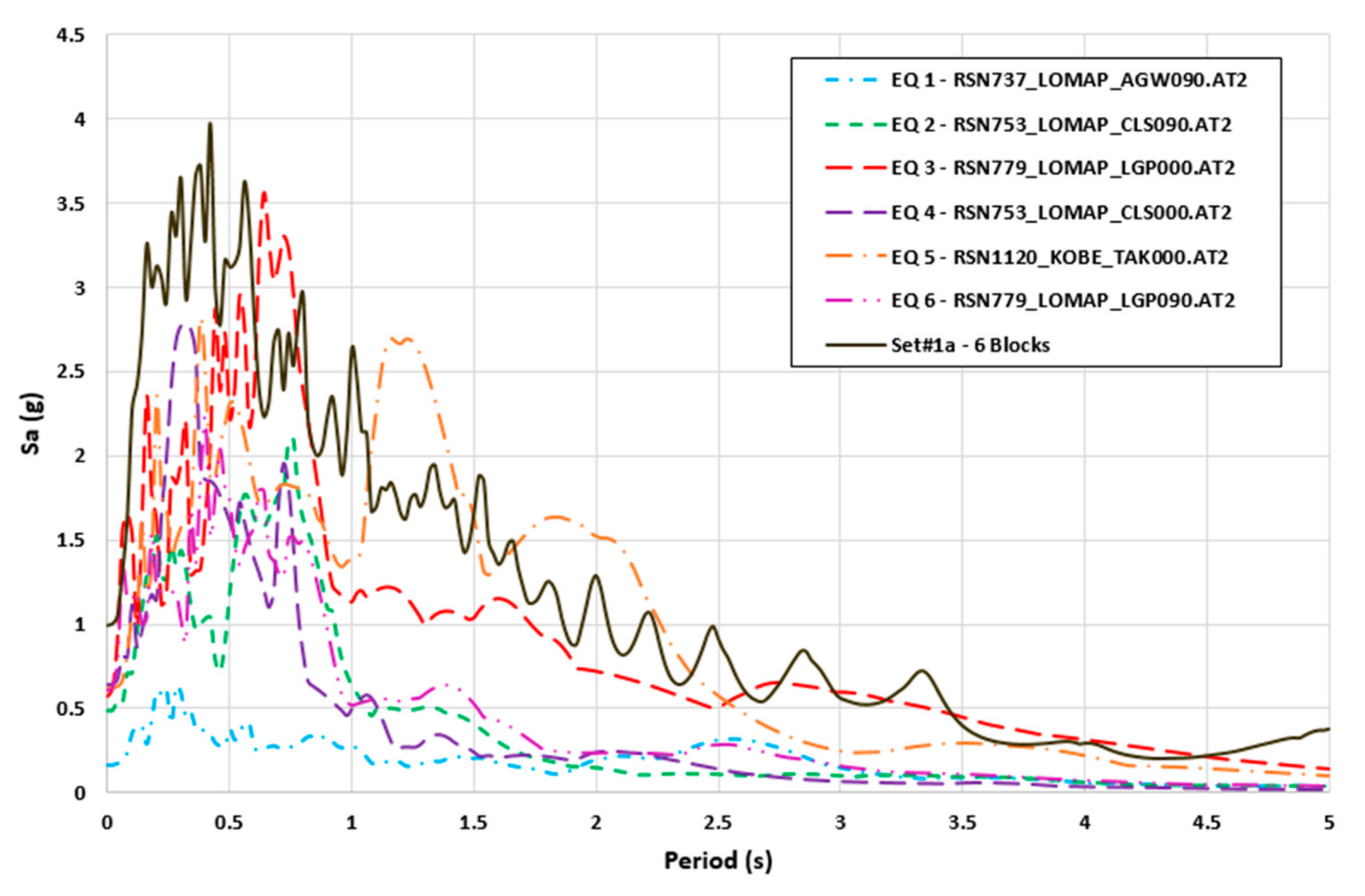
| 737 | Loma Prieta | 18 Oct 1989 | 6.9 | Agnew State Hospital | 90 | 0.161 |
| 753 | Loma Prieta | 18 Oct 1989 | 6.9 | Corralitos | 90 | 0.428 |
| 779 | Loma Prieta | 18 Oct 1989 | 6.9 | LGPC | 0 | 0.569 |
| 753 | Loma Prieta | 18 Oct 1989 | 6.9 | Corralitos | 90 | 0.644 |
| 1120 | Kobe | 16 Jan 1995 | 6.9 | Takatori | 0 | 0.617 |
| 779 | Loma Prieta | 18 Oct 1989 | 6.9 | LGPC | 0 | 0.607 |
| Earthquake Name (Analysis Method) | Run Time (h:min:s) | Output File Size (Kbytes) |
|---|---|---|
| PEER 2015/01 (THA) | 00:46:35 | 119,526 |
| ETEF Set#1a (ETA) | 00:13:19 | 36,139 |
| Improvement | 71.4% | 69.7% |
| Performance Criteria | THA Using the Selected Ground Motions | ETA Using ETEF Set#1a | |||
|---|---|---|---|---|---|
| Criteria | Limit | Time | Value | Time | Value |
| Chord Rotation (IO) | 0.012 | 68.68 | 0.0122 | 44.45 | 0.0122 |
| Concrete Cover damage | −0.0028 | 122.74 | −0.00282 | 62.22 | −0.00281 |
| Spalling | −0.004 | 123.61 | −0.00410 | 6.29 | −0.00404 |
| Chord Rotation (LS) | 0.025 | 123.67 | 0.0258 | 82.31 | 0.0259 |
| Concrete Core | −0.006 | 123.67 | −0.00603 | 82.33 | −0.00610 |
| Chord Rotation (CP) | 0.031 | 123.74 | 0.0312 | 94.77 | 0.0311 |
Disclaimer/Publisher’s Note: The statements, opinions and data contained in all publications are solely those of the individual author(s) and contributor(s) and not of MDPI and/or the editor(s). MDPI and/or the editor(s) disclaim responsibility for any injury to people or property resulting from any ideas, methods, instructions or products referred to in the content. |
© 2023 by the authors. Licensee MDPI, Basel, Switzerland. This article is an open access article distributed under the terms and conditions of the Creative Commons Attribution (CC BY) license (https://creativecommons.org/licenses/by/4.0/).
Share and Cite
Mamaghani, M.; Lui, E.M. Use of Continuous Wavelet Transform to Generate Endurance Time Excitation Functions for Nonlinear Seismic Analysis of Structures. CivilEng 2023, 4, 753-781. https://doi.org/10.3390/civileng4030043
Mamaghani M, Lui EM. Use of Continuous Wavelet Transform to Generate Endurance Time Excitation Functions for Nonlinear Seismic Analysis of Structures. CivilEng. 2023; 4(3):753-781. https://doi.org/10.3390/civileng4030043
Chicago/Turabian StyleMamaghani, Mohammadhossein, and Eric M. Lui. 2023. "Use of Continuous Wavelet Transform to Generate Endurance Time Excitation Functions for Nonlinear Seismic Analysis of Structures" CivilEng 4, no. 3: 753-781. https://doi.org/10.3390/civileng4030043