Investigation of Resonant Signal Timing Plans through Comprehensive Evaluation of Various Optimization Approaches

Abstract

Transportation agencies periodically conduct signal retiming (i.e., optimization) to ensure efficient signal operations. Previous studies introduced the notion of the “resonant cycle length” (RCL), which is based on the premise that a good progression of traffic on the corridor mainline for various volume fluctuations can be achieved with an appropriate value of cycle lengths, where all other signal timing parameters (splits, offsets and phase sequences) remain unaltered. Several follow-up studies brought many inconsistencies in the previously introduced concept. For instance, authors would investigate the existence of the RCL by evaluating the performance of signal timing plans for not only coordinated movements (side streets and coordinated movements together), but would optimize all signal timing parameters (not only cycle lengths) while investigating. This study sheds light on the RCL concept and highlights the importance of all signal timing parameters for signal performance. In addition, we introduce a concept called the resonant signal timing plan (RSTP) as a refinement for the RCL, which represents a combination of signal timing parameters that (unaltered) retain an acceptable performance for a variety of traffic conditions. Results show that different sets of signal timing parameters cause plans to be resonant depending on the evaluation type.

1. Introduction

Signal timing optimization, also known as the signal retiming process, is a widely used strategy to support efficient traffic signal operations. A vast number of studies have been conducted in recent decades to develop the best-performing signal timing plans for prevailing traffic conditions [1,2,3,4,5,6,7]. Emerging technologies, particularly connected and autonomous vehicles, have seemed promising in resolving conflicts at signalized intersections, and would ultimately replace the need for traffic signals and the signal retiming process. However, numerous challenges with this technology’s deployment [8] have been the main reason why a high percentage of traffic signals still requires traditional signal timing optimization to be periodically conducted [9,10,11,12].

In a nutshell, within the signal optimization process, the employed algorithm (i.e., the optimizer) searches for the optimal combination of signal timing parameters, which, when implemented, can reduce various traffic signal performance measures (e.g., delay and number of stops). It can be stated that the main function of signal timing parameters is to accommodate traffic volume as efficiently as possible. The following signal timing parameters are normally considered in optimization: (1) the cycle length—represents the total time to complete one sequence of all movements around an intersection [10]; (2) the green split—represents the amount of time allocated to an individual (movement) within a cycle length [10]; (3) the offset—represents the time between the start of the green indication at one intersection and the start of a green indication at an adjacent/downstream intersection, and defines the movement of traffic along the corridor/major road (also referred to as “progression”) [10]; and (4) the phase sequence—represents the order (of movements) in which phases are served during one cycle [10]. Therefore, all of these parameters play a significant role during the optimization process.

Some time ago, the notion was put forward that one signal parameter, i.e., cycle length, can remain unchanged for a range of traffic volumes and still provide an efficient progression of traffic on the corridor mainline. Such a cycle length was denoted as a “resonant cycle length” (RCL) [13,14]. In that scenario, it was assumed that other signal timing parameters (e.g., offsets and phase sequences) were unchanged, regardless of volume fluctuations. Several follow-up studies investigated whether such a “resonant cycle length” could exist for various traffic conditions and network topologies [15,16,17]. More importantly, researchers expanded the optimization scope to include all signal timing parameters while looking for the RCL [15,16,17]. Such an approach would essentially violate the true definition of the RCL, considering that all parameters are subject to optimization, and yet, only cycle length was denoted as being “resonant”.

Another concern related to the RCL concept and previous studies is the evaluation approach of RCLs. In particular, while evaluating whether cycle length is resonant or not, most of the previous studies evaluated the overall network performance and not just the performance of progressed movements [13,14,15,16,17]. However, the overall network performance includes performance for side-street movements, and there seems to be a disbalance between how the RCL is defined and what constitutes the right measurement of two-way progression. Consequently, previous studies did not provide consistent findings.

Lastly, previous studies showed that not every network topology or traffic volume distribution would result in the existence of such a resonant cycle length [13,14,15,18]. Such an observation is logical, considering the complex interaction between various signal timing parameters, volume distributions and network topologies. However, researchers failed to recognize the importance of all signal timing parameters for efficient signal operations. Therefore, there is a need to recognize the importance and impact of each signal timing parameter on traffic signal performance, or “resonance”.

In this work, the authors shed light on the RCL concept by investigating the impact of other signal timing parameters on signal performance. In particular, the authors look into the overall network performance and the performance of progression (corridor mainline movements), as such a rigorous evaluation has not been previously conducted. We further introduce the resonant signal timing plan (RSTP) concept as a refinement for the RCL, which represents a combination of signal timing parameters that (unaltered) retain an acceptable performance for a variety of traffic conditions. We define the RSTP so broadly on purpose to allow users to: (1) apply this concept for various performance measures (e.g., bandwidth, delays, stops and performance index); (2) define which signal timing parameters should be part of the RSTP; and (3) decide on what is an acceptable level of performance. To study the existence of the RSTP, the authors performed a number of signal timing optimizations on a field-like network and used a couple of different ways to assess the quality of the resulting RSTPs. PTV Vistro [19] was used as a signal optimization program, but the resulting signal timing plans were tested in a calibrated and validated PTV Vissim [20] model, which represented field-like traffic conditions.

2. Research Methodology

To achieve the main objective of this study, we further defined the RSTP for the specific conditions of our study. As the RSTP is defined as “a combination of signal timing parameters that (unaltered) retain an acceptable performance for a variety of traffic conditions”, we discussed what that meant related to the concrete methodology of this study:

• Combination of signal timing parameters—In our study, we optimized all basic signal timing parameters, including the cycle length, offsets, splits and phase sequences. Thus, once an optimization was performed and an optimal signal timing plan was found, which was used without alterations in the testing of all other scenarios. This approach required that experimentation was conducted for alike traffic conditions (e.g., midday balanced flows in each direction, without major shifts of directional traffic demand), but a different approach could be used for different circumstances (e.g., one could consider a RSTP with a fixed cycle length, phasing sequence and splits, while the offsets could be adjusted for the morning and afternoon peaks).
• Acceptable performance—We introduced multiple threshold levels to describe if a RSTP performed similarly to the best signal timing plan (STP) for the given conditions. It is logical that an optimal STP would be the best for conditions for which it was optimized. However, what makes a RSTP distinctive is the fact that a RSTP may be close to the best STPs for many scenarios for which it was not originally designed. In order to classify if a STP can be a candidate for a RSTP, we observed whether its performance was within a threshold (e.g., 5%) of the performance of the best STP. For example, if the best STP for the given conditions could yield a delay of X hours, another STP would be a candidate for the RSTP, for the same conditions, if its performance was within 1.05× hours of delay. Thus, this concept does not recognize only a single RTSP, but a family of RSTPs relevant for the given thresholds, all representing different levels of acceptable performance.
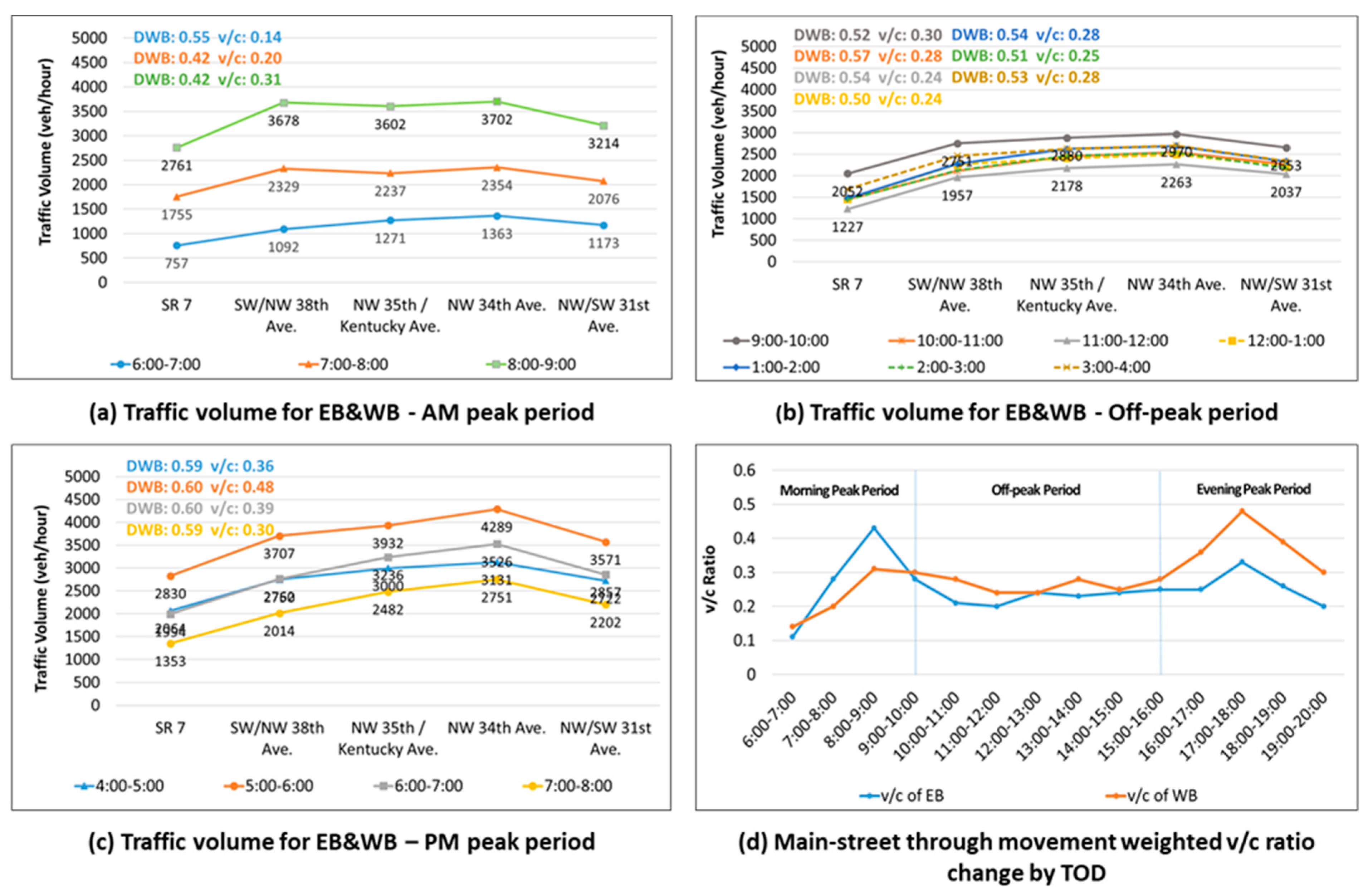
• Variety of traffic conditions—We observed the performance of various STPs over a midday period of several hours when directional traffic flows were balanced to stay truthful to the original idea presented by Shelby et al. [14], where the RCL was defined in such a way.

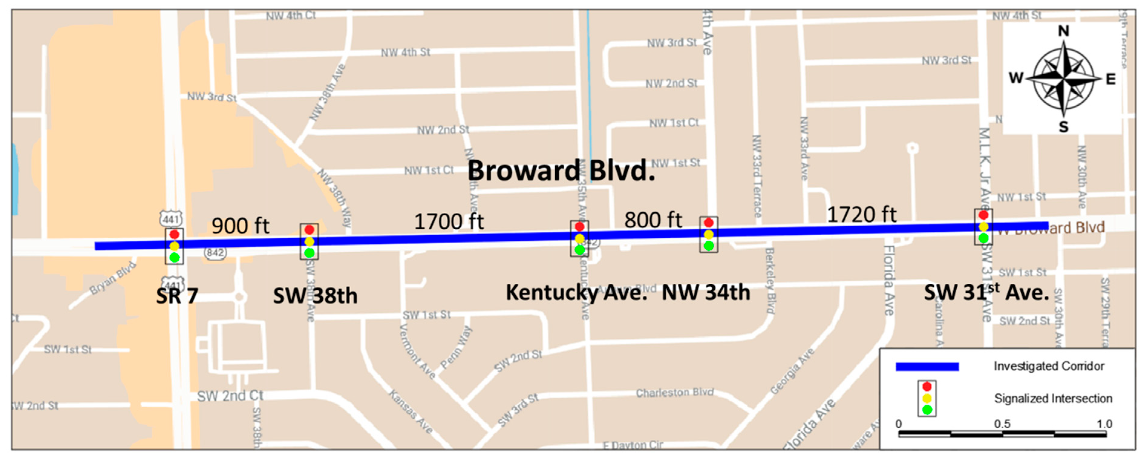
To further explore the behavior of potential RSTPs we organized our evaluation of the (acceptable) performance into two groups: network-level performance (all movements in the network) and coordinated movement performance (only through movements of the coordinated phases). On both levels, the authors used multiple performance measures (average delay, average number of stops, PI and average travel time), which served not only to investigate the existence of RSTPs for specific performance measures, but also of an ‘all-around’ RSTP.

2.1. Study Network

The 5000 ft segment of Broward Boulevard in Ft. Lauderdale, Florida (USA), was selected to conduct the experiments on for this study. The segment encompasses five consecutive signalized intersections (as shown in Figure 1), from SR 7 on the west side to NW 31st Avenue to the east. Among these five intersections, only NW 34th Avenue is a 3-leg intersection with no southbound approach. The spacing between intersections varies from 800 ft to 1720 ft. All of the intersections operate under a fully actuated and coordinated mode with a posted speed limit of 40 mph.

To find out the applicable diurnal period for the RSTP analysis, we partitioned combined directional traffic volumes, as shown in Figure 2, to parts (a), (b) and (c). Three prevailing daily traffic patterns were recognized as follows:

(a)

Pattern 1: from 6:00 to 9:00—morning peak period;

(b)

Pattern 2: from 9:00 to 16:00—off-peak period;

(c)

Pattern 3: from 16:00 to 20:00—evening peak period.

As the Broward Blvd is an east–west arterial sum of EB and WB, through volumes were used to represent the progression volume at each intersection. The direction distribution factor (D factor) and volume-to-capacity (v/c) ratio of the WB direction are also shown in Figure 2. One could observe (from Figure 2d)) that the volumes between 9:00 AM and 4:00 PM represented the most balanced period of the day (as expected); thus, they were selected for the experiments. The reasoning behind this decision was that the very nature of the experiments set for the RSTP required the RSTP to be suitable for multiple traffic conditions. Thus, it is more logical to expect that a RSTP can be found when conditions are alike for multiple hours. In addition to that, the conditions expressed in Figure 2d complied with the requirements for the RST set in previous studies [14].

2.2. Simulation Model Development

The microsimulation models were built in PTV Vissim (v. 9.0) and the macroscopic deterministic models were built in PTV Vistro 2020 (SP 0-0). The development, calibration and validation of the models were challenging and time-consuming tasks, as all the parameters and inputs in the models interacted dynamically. On the other hand, the development of the deterministic models was straightforward and less time-demanding. For hourly periods between 6:00 and 20:00, traffic volumes for this segment were downloaded from the Regional Integrated Transportation Information System (RITIS), and a balance sheet was developed to generate design volumes on the overall network level after balancing, which were then transferred into Vissim. The Florida Department of Transportation (FDOT) provided signal design and timing plan sheets for each intersection, while the speeds were collected from field observations, i.e., travel time runs. Before conducting any experiments in this study, the Vissim/Vistro models were fully calibrated and validated using multiple data sources (i.e., travel times, speeds and occupancy); these efforts were documented in greater detail in a previous study [21].

In a nutshell, for the calibration of the Vissim model, the authors tweaked certain parameters (i.e., the saturation flow rates, desired speed decisions, conflict areas and traffic volume) until satisfactory matching between the modeled volumes, travel times and field data were observed (witnessed with an R² value above 0.8) [21]. Similarly, for the Vistro models, the geometry was coded with the help of the developed Vissim model and Google Maps. The number of left- and right-turn pocket lane lengths was carefully coded to match the field conditions accurately. Estimated turning movement counts were transferred from the balancing spreadsheet to Vistro using special coding (i.e., Python scripts). The duration of signal timing parameters was obtained from Vissim. Saturation flow rates were populated based on values used in the Vissim model. Each link speed was coded based on the posted speed limits. The calibration of the Vistro model was based on traffic volumes (estimated TMCs) and link speeds. In order to ensure that both models processed traffic demands in the same manner, identical values for the saturation flow rates were used. In terms of validation, we compared movement delays reported by the Vistro model (based on HCM10 methodology) and Vissim model (obtained from .knr file), and once a desirable level of correlation was achieved (R2 higher than 0.8), the model was considered validated.

2.3. Experimental Design

For the purpose of testing the existence of the RSTP, the authors selected 5 different optimization scenarios based on the optimization options available in PTV Vistro. Each of those 5 optimization scenarios were then used to optimize the signal timings for traffic for each hour during the midday period between 9:00 and 16:00 h. In addition to the five new optimizations, the authors also investigated the performance of the existing field signal timings, denoted as the base case scenario in the remainder of the paper. Differences between all of the signal optimization scenarios are shown in

Table 1. Comparison of field signal timing plan and 5 optimization approaches.

Scenario	Optimization Mode	Cycle Length	Split	Offsets	Phase Sequence
LoCwSPr	Locally	Yes	No	No	No
LoCS	Locally	Yes	Yes	No	No
NoCS	Network	Yes	Yes	No	No
NoCSO	Network	Yes	Yes	Yes	No
NoCSOPs	Network	Yes	Yes	Yes	Yes

, while specific descriptions are given below:

• Local cycle length optimization with splits proportionally (LoCwSPt) distributed: After Local optimization of splits and cycle times for each intersection, the longest cycle length was selected for the entire network, and the intersections’ splits were adjusted proportionally. This optimization strategy aimed to find the optimal cycle length (between 30 and 200 s) for each intersection by using the local optimization function in PTV Vistro. The largest cycle length of those five was chosen as the cycle length of the whole network and the intersection splits were increased proportionally. The optimization objective function was to minimize the critical movement delay.
• Local cycle length and splits (LoCSs) optimization: After the local optimization of splits and cycle times for each intersection, the longest cycle length was selected for the entire network and the intersections’ splits were again optimized with Vistro.
• Network cycle length and splits (NoCSs) optimization: In this scenario, Vistro’s network optimization was used to find the optimal cycle length and splits. The performance index (PI) was used as an objective function with a stop penalty of 8, the same value as used in the study of Shelby et al. [14]. Hill climbing was chosen as a search mechanism and the number of starting solutions was set to 20.
• Network cycle length, splits and offsets (NoCSOs) optimization: This scenario was similar to NoCS, but the offset optimization was added to the options for network optimization, which meant that the cycle length, splits and offsets were all optimized on the network level.
• Network cycle length, splits, offsets and phase sequences (NoCSOPs) optimization: In this scenario, phase sequence optimization was added to the optimization options. All other settings remained the same as in NoCSO.

After performing 5 optimization scenarios for each of the hourly volumes (from 9 AM to 4 PM), all of the signal timing plans were imported into the relevant PTV Vissim models. Essentially, all of the Vissim models were the same in terms of the geometry and driving characteristics except for their traffic demands (to reflect midday hourly volumes) and signal timing plans, reflecting various signal optimization scenarios. There were, in total, 36 different Vissim files, which were run with 10 random seeds to achieve the necessary stochasticity of the results.

2.4. Evaluation Procedure

All of the signal timing scenarios were evaluated based on the same four performance measurement (average delay, average stops, PI value and average travel time), which were deliberately chosen to be similar to performance measures used in previous studies [13,14]. In this way, findings from this study could be more relevant for comparison with the findings from previous research works.

By definition, a RSTP would be one that had the best performance (whichever performance measure was chosen) for all of the hourly intervals during the midday period. Considering that this was not likely to be the case, we introduced the concept of a STP being within an acceptable performance threshold of the optimal STP for a specific period. Then, a RSTP would be, logically, a STP that was ranked the best among all of the competing plans. To ensure that we could capture the existence of RSTPs for multiple thresholds, we arbitrarily introduced a number of thresholds from 3 to 20% (3%, 5%, 10%, 15% and 20%). For instance, 3% meant that the performance of the STP during the examined period was within 3% of the best performance achieved by other (not necessarily the same) STPs during the examined period. Logically, a separate RSTP would be sought for each performance measure, although it was expected that some significant overlapping may exist. Finally, it is important to remind readers that all of the STPs were developed in Vistro, but evaluated in Vissim, which created a situation similar to many field-like evaluations when something developed by a model does not necessarily ‘work’ in reality; only, in this case, the microscopic models from Vissim took a role of recreating realistic conditions. The flowchart illustrated in Figure 3 shows the study approach introduced in this section.

3. Results and Discussion

This section consists of two subsections, where the results of the proposed optimization approaches were documented on two levels: the overall network (i.e., all movements) and corridor mainline (i.e., coordinated movements). Findings about resonant signal timing plans for each evaluation approach were provided within their own sections.

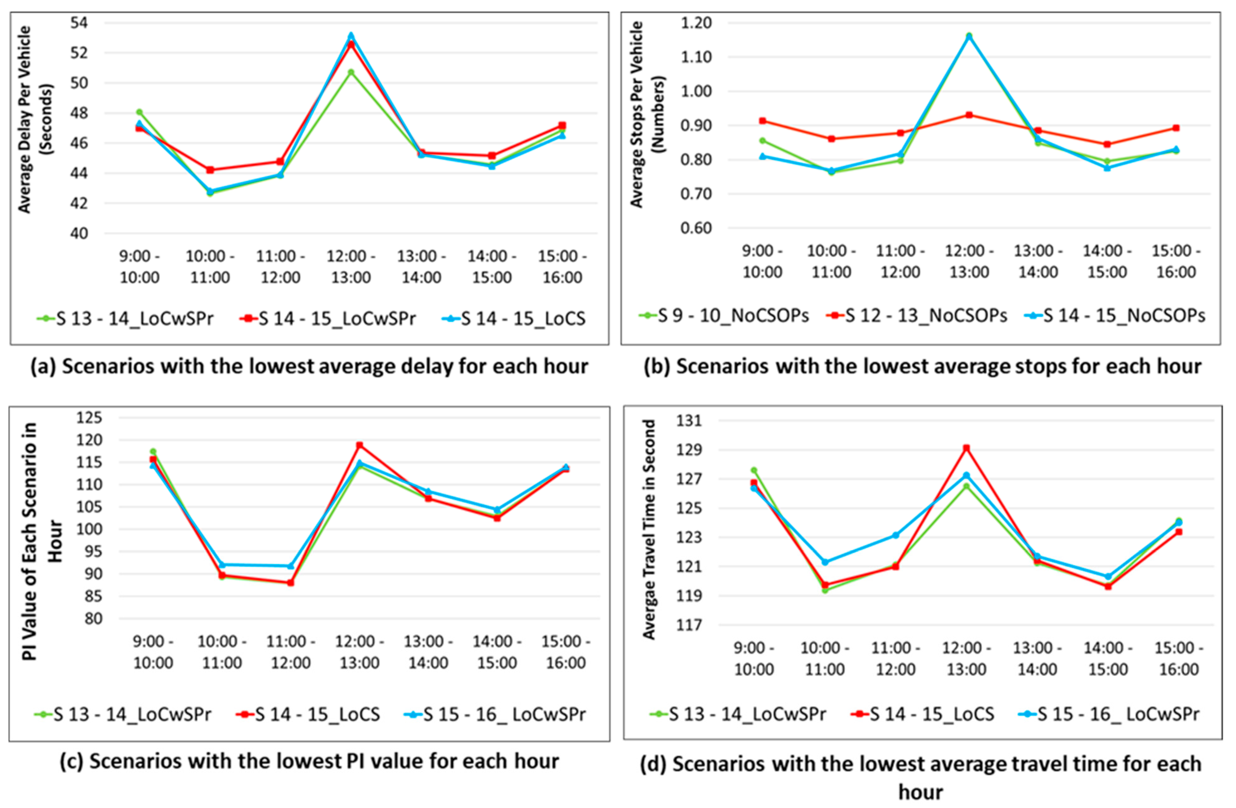
3.1. Network Evaluation

Figure 4 shows the performance measures average delay and average number of stops from all of the 35 scenarios considered under the network evaluation. As discussed in previous sections, for each of the examined hours (e.g., from 9 to 10), sets of signal timing plans (i.e., five) were developed and each of those developed signal timing plans were set to operate for whole examined periods (i.e., from 9 to 16) in order to investigate the plan resonance. Please note that the examined performance measures for the existing signal timing plans (deployed in the field) were denoted as “Field” in Figure 4. It can be stated that, in general, across all performance measures, signal timing optimization was successful in reducing performance measures when compared to field timings. However, in some instances, the optimization tool failed to generate better-performing signal timing plans (when compared to field plans). The authors found limitations in Vistro as the main reason for such results, and these results were aligned with some of our previous studies [22]. For the sake of brevity, the authors omitted the presentation of results for PI and the average travel time, as they followed similar trends as the average delay and average number of stops. It needs to be pointed out that Figure 4 serves to present all the results to allow to spot general trends and very mixed results on a scenario and hourly basis. Considering that the study’s main purpose was to investigate the best-performing STPs, we extracted those optimization scenarios for all four performance measures that reported the best performance during the examining period. These results are shown in Figure 5.

Under the average delay evaluation (Figure 5a), the best plan between 9:00 and 10:00 was the optimal STP for “LoCwSPr 14-15”. Then, from 10:00 to 14:00, the optimal STP was “LoCwSPr 13-14”. Finally, from 14:00 to 16:00, the best results were achieved with the optimal STP “LoCS 14-15”. According to the results, a single best STP to provide the lowest average delay for all 7 h, under the network evaluation, was not discovered. Interestingly, the three optimal STPs, which were best for parts of the 7 h period, were all based on the local optimization scenarios where only cycle lengths and/or splits were optimized, and offsets or phase sequences were not optimized.

When evaluating the average number of stops (Figure 5b), it could be concluded that all scenarios that yielded minimal average stops were different from those that yielded the lowest average delays. For instance, from 9:00 to 10:00 and 14:00 to 15:00, the optimal STP “NoCSOPs 14-15” was the best. From 10:00 to 12:00, 13:00 to 14:00 and 15:00 to 16:00, the optimal STP “NoCSOPs 9-10” was the one with the lowest average stops. Similarly, for the period from 12:00 to 13:00, the optimal STP “NoCSOPs 12-13” provided the best stopping performance among all 36 STPs. Similar to the findings of average network delays, due to the mixed performance of the investigated STPs, there was no single best STP. However, the three best STPs for the average stops all included the full network optimization of all signal timing and phasing parameters.

The results drawn from the PI evaluation (Figure 5c) showed that from 9:00 to 10:00, the optimal STP “LoCwSPr 15-16” yielded the lowest PI. Between 10:00 and 14:00, the best optimal STP was “LoCwSPr 13-14”. For the remaining 2 h, scenario “LoCS 14-15” was found to be the one with the lowest PI value. Similar to previous evaluations, no single STP reached the lowest PI value for all 7 h when the PI was considered for the network evaluation. The three best STPs for individual hours were similar to the ones selected in the average delay evaluations, which was not a surprise, considering that delay was an integral part of the PI.

For the average travel time evaluation (Figure 5d), it could be observed that from 9:00 to 10:00, the optimal STP was “LoCwSPr 15-16”, with the shortest average travel time. From 10:00 to 11:00 and 12:00 to 14:00, the best STP was one developed as “LoCwSPr 13-14”. From 11:00 to 12:00 and 14:00 to 16:00, scenario “LoCS 14-15” was the best one, with the lowest average travel time. It was interesting to notice that these three optimal STPs were the same as the best ones found for the network level’s PI. Only a slight difference occurred for the period between 11:00 and 12:00, as the average travel time of scenario “LoCwSPr 13-14” was negligibly lower than that of “LoCS 14-15”. Similar to the previous cases, there was no indication that any of the investigated STPs showed superior performance over the entire 7 h period. However, the fact that some of the STPs yielded both the lowest PI value and the shortest average travel time was encouraging.

In summary, based on the results of four performance measures of the network level evaluation, it could be concluded that no single STP performed the best for the entire experimental period in the study network. However, two optimal STPs, for “13:00–14:00” and “14:00–15:00”, frequently appeared as the STPs that could provide the best performance for a number of hours and performance measures. It was also noticeable that the cycle lengths of these two STPs were very similar—132 and 133 s, respectively. Considering that the cycle lengths were often defined in 5 s increments, one could claim that these two actually represented the same cycle length that could be defined as an RCL of the study network. However, a sole value of cycle length is not sufficient enough to properly represent coordinated traffic signal operations, because the splits, offsets, phase sequences, etc., are all important elements that should also be taken into consideration when setting optimal signal timings.

Although there was no STP that could be identified as the best one, several optimal STPs had the potential to be identified as RSTPs if their performance could fit in a specific acceptable threshold. For example, if we set an acceptable threshold of 3%, scenario “LoCwSPr 13-14” could be identified as a RSTP for three out of four of the investigated performance measures (except for average stops). Similarly, for a 5% acceptable threshold, the number of RSTPs increased to four STPs, while none of them still included average stops. Similarly, seven optimal STPs could be identified as RSTPs if the threshold was increased to 10%, etc. The first time that some STPs could be identified as RSTPs for all of the investigated performance measures would be if we were to increase the threshold to 20%. In that case, scenarios “LoCwSPr 12-13” and “LoCwSPr 15-16” would be two STPs identified as RSTPs for all four performance measures.

Table 2. Potential RSTPs within a certain threshold under network-level evaluation.

Threshold	Scenario
3%	S 13-14 LoCwSPr
5%	S 13-14 LoCwSPr	S 14-15 LoCS	S 14-15 LoCwSPr	S 15-16 LoCwSPr
10%	S 13-14 LoCwSPr	S 14-15 LoCS	S 14-15 LoCwSPr	S 15-16 LoCwSPr	S 13-14 LoCS
	S 15-16 LoCS	S 12-13 LoCwSPr
15%	S 13-14 LoCwSPr	S 14-15 LoCS	S 14-15 LoCwSPr	S 15-16 LoCwSPr	S 15-16 LoCS
	S 12-13 LoCwSPr	S 13-14 LoCS	S 11-12 LoCwSPr
20%	S 13-14 LoCwSPr	S 14-15 LoCS	S 14-15 LoCwSPr	S 15-16 LoCwSPr	S 13-14 LoCS
	S 15-16 LoCS	S 12-13 LoCwSPr	S 11-12 LoCwSPr	S 11-12 LoCS	S 12-13 LoCS

shows all of the RSTPs identified based on scenarios that consistently provided good performance regarding the average delay, PI and travel time.

In spite of the inconsistencies related to the average number of stops, the STP “LoCwSPr 13-14” could be identified as an all-round RSTP, for the network evaluation, as it performed better than other STPs within the entire range of thresholds from 3% to 20%. In addition, no matter how high or low the threshold was set, most of the potential RSTPs were based on local optimizations, which meant that the offsets and phase sequences remained the same as those in the field. Therefore, these findings raised the question of whether the network level evaluation in Vistro is a suitable method for studying the existence of RSTPs. As a consequence of this finding, one could raise the question of whether the previous studies, which also used network-wide performance measures, had delivered trust-worthy results for the identification of the RCL. Table 2 shows STPs that provided reasonably good performance for the entire 7 h period and for every performance measure used to evaluate the entire network.

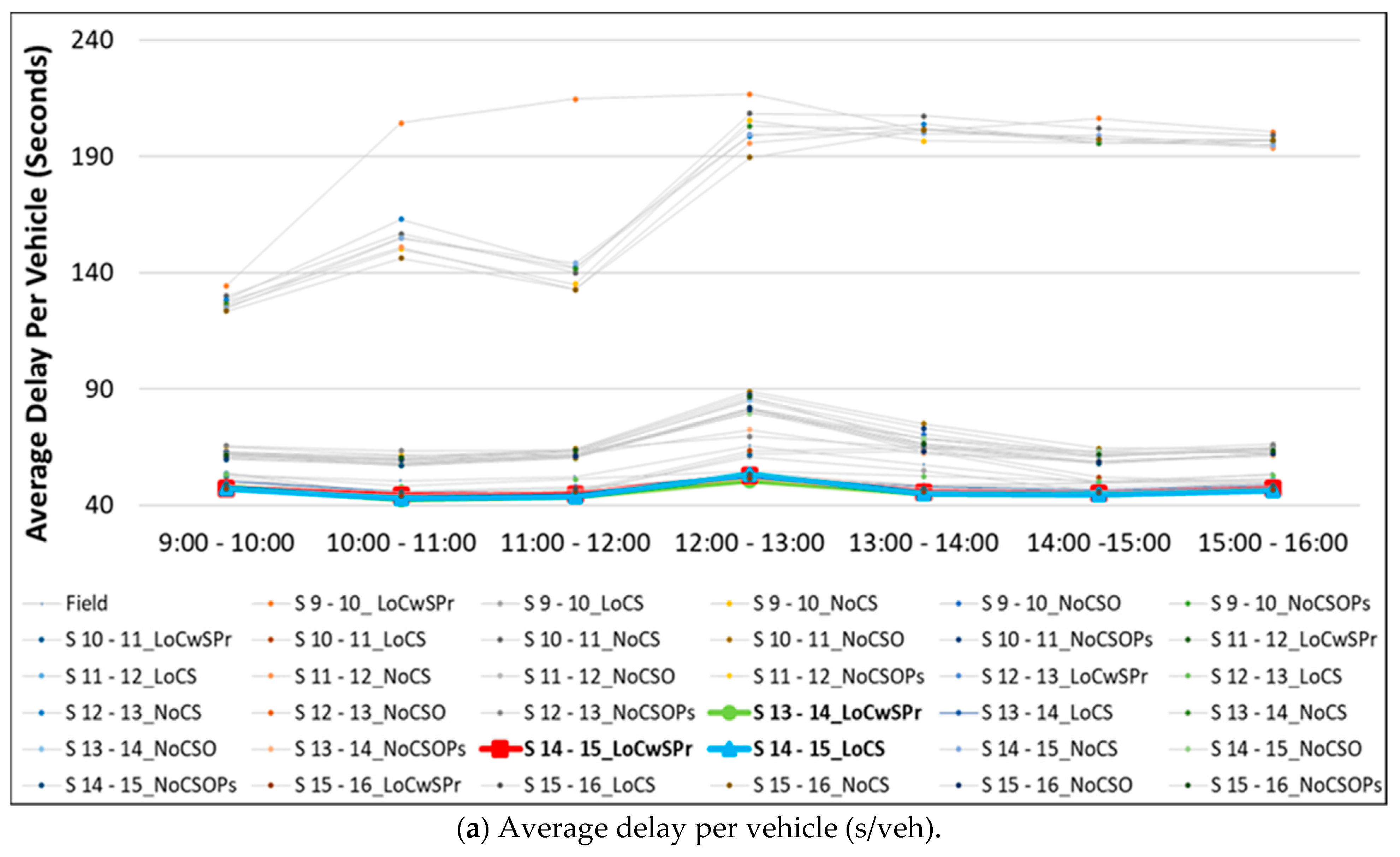
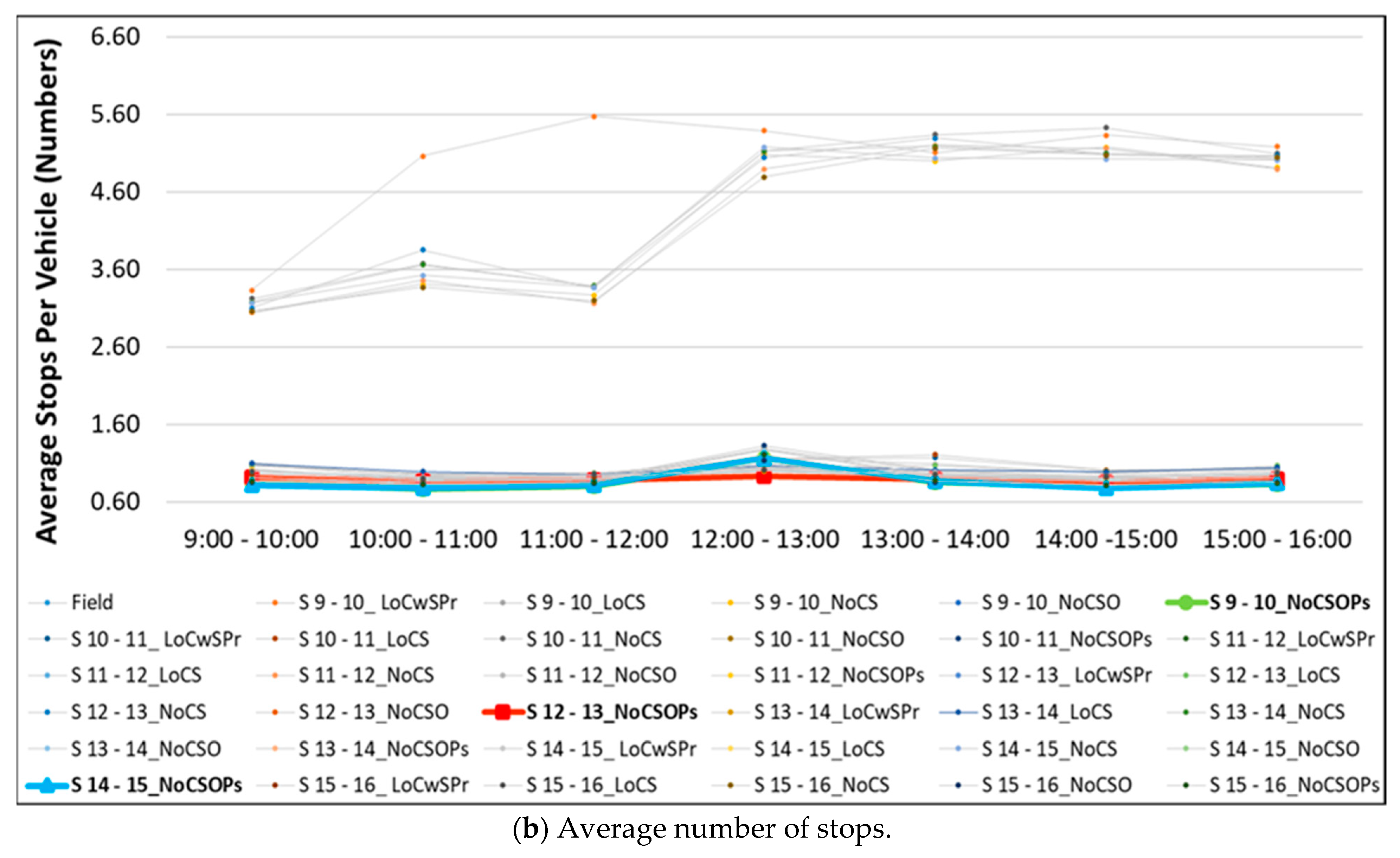
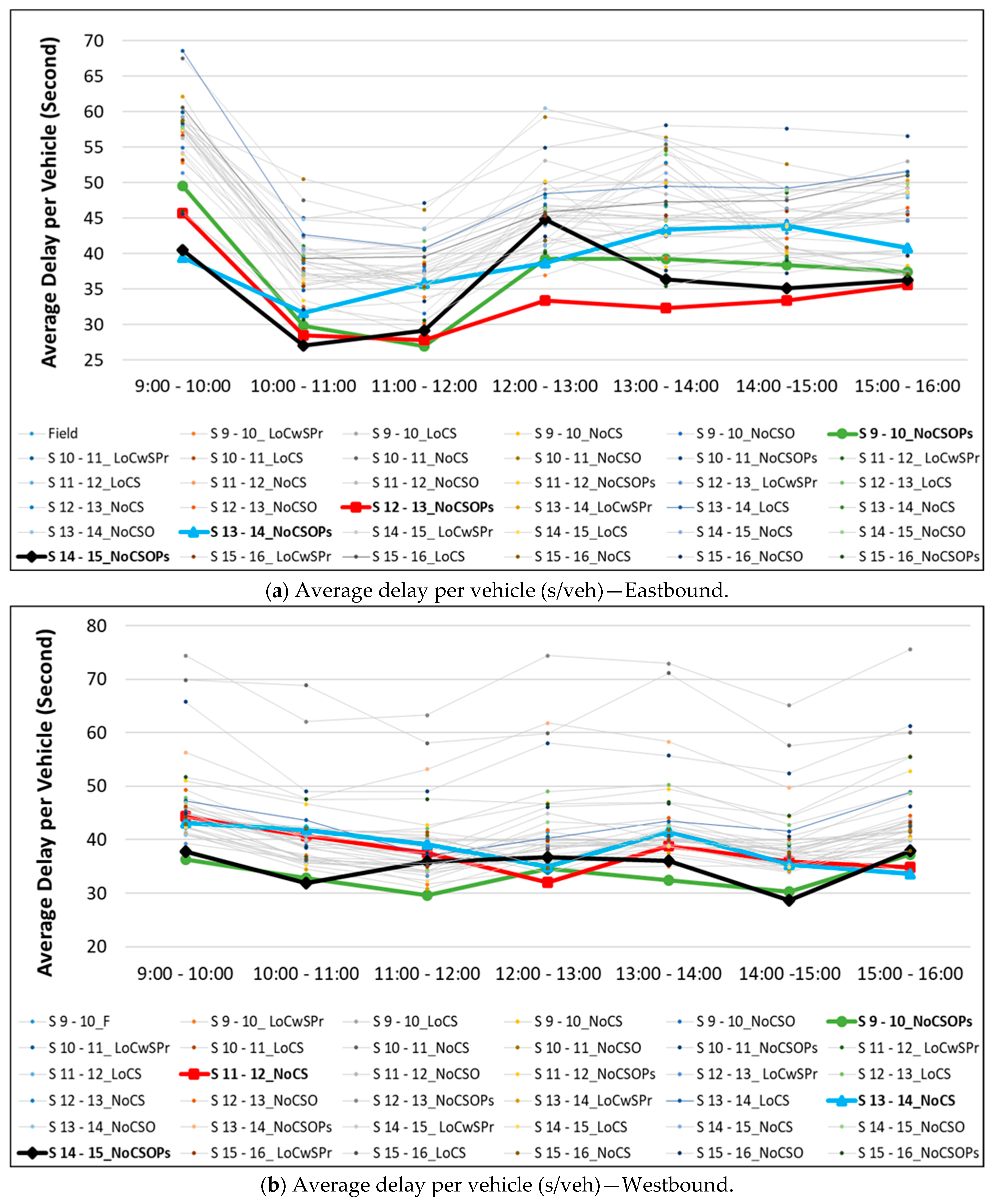
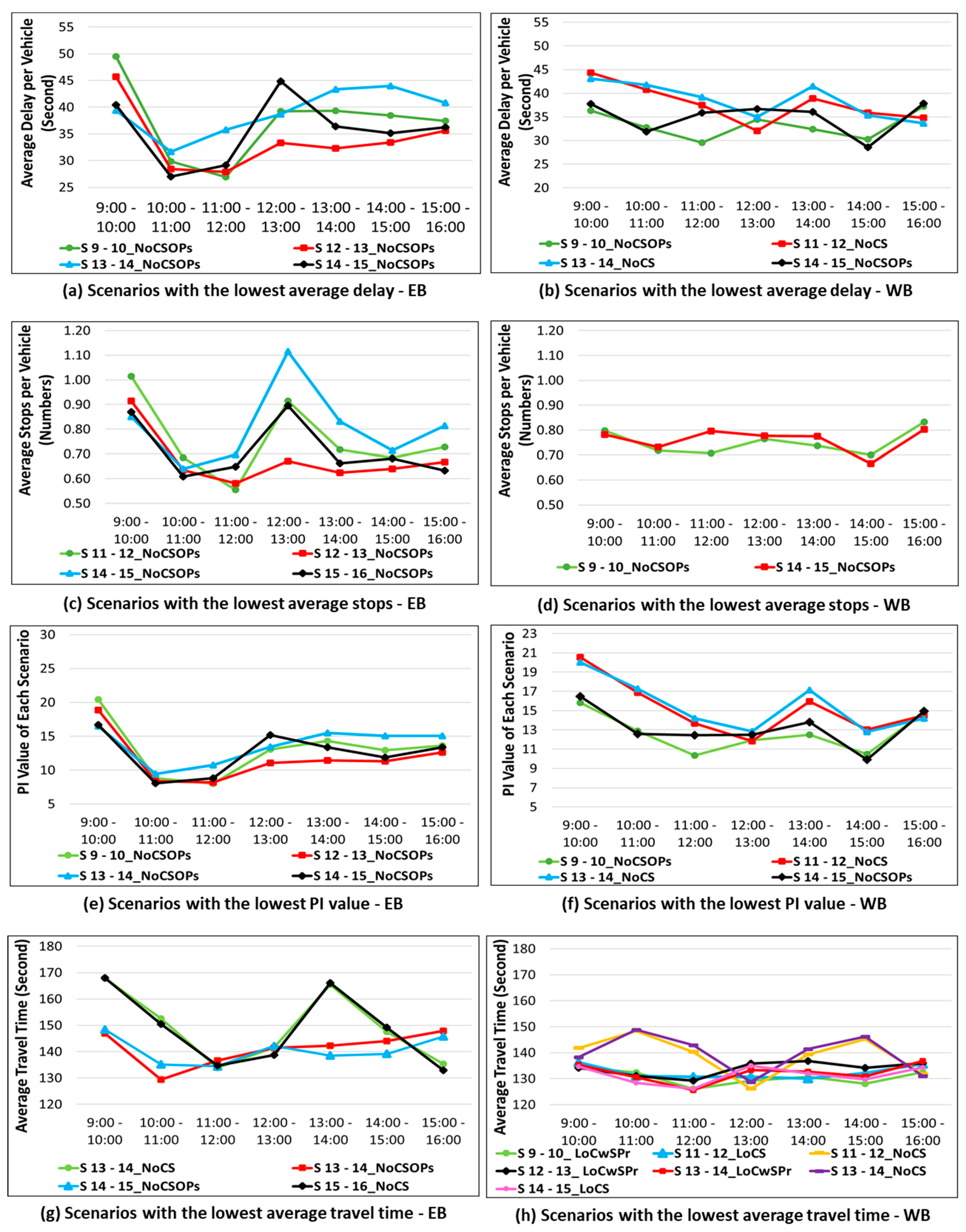
3.2. Progression Evaluation

As discussed earlier, another objective of this study was to document the performance of only eastbound (EB) and westbound (WB) coordinated through traffic to avoid a similar problem seen in previous studies, where the RCL, which is supposed to provide good two-way progression, was evaluated for the entire network and not only for progressed movements [13,14,15,16,17]. The performance measures used in this evaluation were still the same as in the network evaluation presented above, but they were aggregated only for the main-street through movements. Figure 6 shows the results of such evaluations for the EB and WB directions for average delays. Similar to the previous section, the authors omitted the presentation of the average number of stops, PI values and average travel times. Although high variations in performance measures and between observed movements were recorded, consistent fluctuations between EB and WB directions were observed.

The reader is reminded that Figure 6 serves to present all results to allow to spot general trends and very mixed results on a scenario and hourly basis. Considering that the study’s objective was to look into the best-performing STPs across a range of traffic volumes and for various performance measures, the authors extracted the best-performing STPs, with the results reported in Figure 7.

Figure 7a,b shows the performance of various optimal STPs for the average delay. The findings showed that none of the 36 STPs could be identified as the best plan for all 7 h, either for progressed movements in the EB or WB direction. All of the best STPs for the EB direction were based on the optimization of all signal timings and phasing parameters. The “NoCSOPs 12-13” scenario could be identified as a potential RSTP as it yielded the lowest average delay for 4 h (12:00–16:00). For the WB direction, the optimal STP for the period between 9:00 and 10:00 was the best potential RSTP, as it performed best during three 1 h periods.

For the average stops evaluation (shown in Figure 7c,d), there was also no single STP that could yield minimal average stops for all 7 h, for either direction. One thing that should be noted about the results for average stops was that all of the best STPs were obtained from optimizations that included all of the signal timing and phasing parameters. Similar to the results for average delays, a STP developed for the period between 12:00 and 13:00 (“NoCSOPs 12-13”) had the potential to be identified as a RSTP, for the EB progression, as it consistently provided the lowest average stops for 3 h. Similarly, STP “NoCSOPs 9-10” was the one identified as a RSTP for the WB progression, where it was dominant for 4 h.

The PI evaluations (shown in Figure 7e,f) showed very similar trends as the evaluations of average delays; obviously, the contribution of stops in the PI was smaller than that of the delays. There was no STP to show consistent supremacy over the entire 7 h period, either in the EB or WB direction. Most of the best STPs were, again, based on the optimization of all signal timings and phasing parameters, with two exceptions for the WB direction. A STP developed for the period between 12:00 and 13:00 could be identified as a RSTP for the EB direction, with the lowest PI for 4 h between 12:00 and 16:00. For the WB direction, an optimal STP for the period between 9:00 and 10:00 was identified as a RSTP, as it performed best for three 1 h periods.

The results for the evaluations of average travel times were not much different from the other performance measures. Again, there was no single STP, either for the EB or WB direction, to yield the shortest average travel time for the entire 7 h period, as shown in Figure 7g,h. All of the best STPs were based on network optimizations (although not always were all timing and phasing parameters optimized) and a single STP was never the best for longer than 2 h within the 7 h period. For the WB progression, there was no apparent trend to recognize any of the STPs being capable of emerging as a RSTP. This evaluation scenario was the most random of all, with every hour having a different best STP, many of which were results of local optimizations.

In summary, there was not a single STP that could be identified as a RSTP for all 7 h and all of the evaluated performance measures. Moreover, the optimal STPs developed with the goal to improve progressed movements (for all performance measures, except average stops) were significantly distinctive from those that were optimal for the network evaluations. While the potential RSTPs based on the network evaluations were all results of local optimizations (which did not include the optimization of offsets and phase sequences), the analysis of progressed movements showed that all of the potential RSTPs benefitted from the network optimization.

According to the results of the EB evaluations for average delays, stops and PI values, the STP developed for the period between 12:00 and 13:00 (when all signal timing and phasing parameters were optimized) consistently provided the best performance for 3–4 h. However, that STP was not identified as being resonant for average travel times, as the results showed that no STP performed as the best one for more than 2 h. For the WB progression, the best STP was one developed for the period between 9:00 and 10:00, when, again, all of the signal timing and phasing parameters were optimized. This STP was the best in terms of the average delay, average stops and PI values, and it provided consistent performance for more than 3 h. Similar to the EB progression, this STP (although potentially resonant for other performance measures) failed to prove its resonance for average travel times.

Similar to the network evaluation, potential RSTPs were found under some of the proposed thresholds. The RSTPs could not be identified for thresholds of 3% and 5%, either for the EB or WB direction. When the threshold was increased to 10%, two different STPs (one for EB, the other for WB) emerged as RSTPs for a number of stops during the entire 7 h period, but failed to emerge as being resonant in terms of other performance measures. The STP “NoCSOPs 12-13” was found to be resonant for the EB progression when the thresholds were 15% and 20%. For the WB progression, a STP developed for 9:00–10:00, when all signal timing and phasing parameters were optimized, was found to be resonant under thresholds of 15% and 20%. Finally, the STP “NoCSO 11-12” was found to be a RSTP for a 20% threshold. Although there were many STPs that appeared to be resonant in terms of the average travel times, they were not found to have even near-resonant performance for other types of performance measures, which meant that the average travel time did not work consistently with the other investigated measures.

Table 3. Potential RSTPs for various thresholds under progression evaluation.

Threshold	Scenario
	Eastbound	Westbound
3%	NA 1	NA
5%	NA	NA
10%	NA	NA
15%	S 12-13_NoCSOPs	S 9-10_NoCSOPs
20%	S 12-13_NoCSOPs	S 9-10_NoCSOPs	S 12-13_NoCSOPs

¹ Not applicable (NA).

shows scenarios that provided resonantly good performance for the entire 7 h period for every performance measure used to evaluate the progressed movements.

For the analysis of progressed movements, the minimum threshold to define a RSTP (for either direction) was 15%, which was much higher than the one observed when the performance was evaluated on the network level. This finding could be explained by the nature of the intended optimizations. While it was quite difficult for a STP to provide good progression in both directions, when it came to the network performance, it may have been easier to justify that a STP could provide various benefits for different movements in the network during multiple hours. Simply put, the goal of a STP for network-wide optimal performance is less specific (than the one for optimal progression), which may make it more resonant. Thus, a truly resonant STP for good bidirectional progression (which would fit in narrow thresholds of the optimal performances, for every measure and every hour) may not exist. In addition, unlike the results obtained for the network evaluations, all the RSTPs for progressed movements benefited from network-wide optimizations, which included adjustments in offsets and phase sequences. Thus, a progression-level evaluation, which used the performance measures aggregated only for the main-street through movements, may be a more reasonable approach for assessing the bidirectional nature of resonant signal timing plans than a network-level evaluation.

4. Conclusions

This study provided a comprehensive analysis of the resonance of signal timing plans developed for arterial coordinated signal control. The study started with the premise that the concept of the so-called “resonant cycle length” should be modified with a new concept called the “resonant signal timing plan”, because cycle length alone cannot be used to classify the coordination of traffic signals. Parameters, such as the split, offset and phase sequence, must be considered at the same time. Ideally, a signal timing plan would be resonant if it was best in all aspects (all performance measures) for all time periods. However, since such an outcome is highly unlikely, there is a need to redefine the definition of the resonant signal timing plan as one that is the closest possible to the performance of the best signal timing plan for as many performance measures and as many periods as possible.

The results from the network evaluation were entirely different from those of the evaluation of the progressed movements, as the charts of the equivalent performance measures never showed similar patterns. Most of the optimal signal timing plans under the network evaluation did not benefit from network optimization, which would include adjustments in the offsets and phasing sequences. For the progressed movements, the majority of optimal signal timing plans were based on the network-wide optimization of all signal timing and phasing parameters.

The findings, thus, questioned whether a network-level evaluation is a suitable approach for the determination/identification of resonant signal timing plans. The side-street delays and stops are as important as those on the main-street, but they usually do not ‘drive’ the determination of the cycle length, offsets and phase sequences, which are all parameters that control main-street progression. Additionally, for this particular model (maybe the fact that PTV Vistro was used mattered too), it did not seem that network-level optimization (of the cycle length, offset, and phase sequence) had a significant impact on the network-level evaluation. On the other hand, the evaluation of the progressed movements seemed more appropriate for investigating the resonant signal timing plans. The reader is reminded that the findings in this study were based on an extensive evaluation of one real-world corridor. In the future, the proposed method can be applied to different network topologies and geographical regions to solidify the obtained conclusions. Additionally, the proposed approach could be tested for a variety of traffic signal performance measures [23], encompassing environmental effects [24,25,26], safety [27,28,29] and multiple users [30,31,32].

References

1. Gartner, N.; Little, J.D.; Gabbay, H. Optimization of traffic signal settings in network by mixed-integer linear programming. Transp. Sci. 1974, 9, 344–363. [Google Scholar] [CrossRef]
2. Foy, M.D.; Benekohal, R.F.; Goldberg, D.E. Signal timing determination using genetic algorithms. Transp. Res. Rec. 1992, 108. [Google Scholar]
3. Hu, P.; Tian, Z.Z. A new approach to variable-bandwidth progression optimization. In Proceedings of the Transportation Research Board 89th Annual Meeting, Washington, DC, USA, 10–14 January 2010. No. 10-1140. [Google Scholar]
4. Stevanovic, J.; Stevanovic, A.; Martin, P.T.; Bauer, T. Stochastic optimization of traffic control and transit priority settings in VISSIM. Transp. Res. Part C Emerg. Technol. 2008, 16, 332–349. [Google Scholar] [CrossRef]
5. Shayeb, S.A.; Dobrota, N.; Stevanovic, A.; Mitrovic, N. Assessment of arterial signal timings based on various operational policies and optimization tools. Transp. Res. Rec. 2021, 2675, 195–210. [Google Scholar] [CrossRef]
6. Shirke, C.; Sabar, N.; Chung, E.; Bhaskar, A. Metaheuristic approach for designing robust traffic signal timings to effectively serve varying traffic demand. J. Intell. Transp. Syst. 2022, 26, 343–355. [Google Scholar] [CrossRef]
7. Dobrota, N.; Mitrovic, N.; Gavric, S.; Stevanovic, A. Comprehensive Data Analysis Approach for Appropriate Scheduling of Signal Timing Plans. Future Transp. 2022, 2, 27. [Google Scholar] [CrossRef]
8. Korosec, K. Ford, VW-backed Argo AI is Shutting Down. TechCrunch+. 26 October 2022. Available online: https://techcrunch.com/2022/10/26/ford-vw-backed-argo-ai-is-shutting-down/ (accessed on 19 December 2022).
9. Gordon, R.L. Traffic Signal Retiming Practices in the United States; Transportation Research Board: Washington, DC, USA, 2010. [Google Scholar]
10. Urbanik, T.; Tanaka, A.; Lozner, B.; Lindstrom, E.; Lee, K.; Quayle, S.; Beaird, S.; Tsoi, S.; Ryus, P.; Gettman, D.; et al. Signal Timing Manual; Transportation Research Board: Washington, DC, USA, 2015. [Google Scholar]
11. Dobrota, N.; Stevanovic, A.; Mitrovic, N. Development of assessment tool and overview of adaptive traffic control deployments in the US. Transp. Res. Rec. 2020, 2674, 464–480. [Google Scholar] [CrossRef]
12. ITE. Traffic Signal Benchmarking and State of the Practice Report; ITE: Washington, DC, USA, 2020; pp. 39–43. [Google Scholar]
13. Henry, R.D. Signal Timing on a Shoestring; U.S. Department of Transportation, Federal Highway Administration: Washington, DC, USA, 2005. [Google Scholar]
14. Shelby, S.G.; Bullock, D.M.; Gettman, D. Resonant Cycles in Traffic Signal Control. Transp. Res. Rec. J. Transp. Res. Board 2005, 1925, 215–226. [Google Scholar] [CrossRef]
15. Guevara, F.L.; Hickman, M.; Head, L. Resonant Cycles under Various Intersection Spacing, Speeds, and Traffic Signal Operational Treatments. Transp. Res. Rec. J. Transp. Res. Board 2015, 2488, 87–96. [Google Scholar] [CrossRef]
16. Guevara, F.L. Resonant Cycles and Traffic Signal Performance; The University of Arizona: Tucson, AZ, USA, 2013. [Google Scholar]
17. Day, C.M.; Emtenan, A.M.T. Impact of Phase Sequence on Cycle Length Resonance. Transp. Res. Rec. J. Transp. Res. Board 2019, 2673, 398–408. [Google Scholar] [CrossRef]
18. Li, H.; Day, C.; Hainen, A.; Stevens, A.; Lavrenze, S.; Smith, B.; Summers, H.; Freije, R.; Sturdevant, J.; Bullock, D. Field Cycle Length Sweep to Evaluate Resonant Cycle Sensitivity. JTRP Other Publications and Reports. Paper 8. 2014. Available online: https://docs.lib.purdue.edu/jtrpdocs/8/ (accessed on 19 December 2022). [CrossRef] [Green Version]
19. PTV-Vision, PTV Vistro 2020 User Manual. 2019. Available online: https://www.ptvgroup.com/en/solutionsproducts/ptv-vistro/ (accessed on 3 April 2019).
20. PTV-Vision, PTV Vissim 2020 User Manual. 2019. Available online: https://www.ptvgroup.com/en/solutionsproducts/ptv-vissim/ (accessed on 5 March 2019).
21. So, J.; Ostojic, M.; Jolovic, D.; Stevanovic, A. Building, Calibrating, and Validating a Large-scale High Fidelity Microscopic Traffic Simulation Model-A Manual Approach. In Proceedings of the 95th Annual Meeting of the Transportation Research Board, Washington, DC, USA, 10–14 January 2016. [Google Scholar]
22. Dobrota, N.; Stevanovic, A.; Mitrovic, N. Modifying signal retiming procedures and policies by utilizing high-fidelity modeling with medium-resolution traffic data. Transp. Res. Rec. 2022, 2676, 660–684. [Google Scholar] [CrossRef]
23. Gavric, S.; Dobrota, N.; Erdagi, I.; Stevanovic, A.; Osman, O. Estimation of Arrivals on Green at Signalized Intersections Using Stop-Bar Video Detection. Transp. Res. Rec. 2023. [Google Scholar] [CrossRef]
24. Erdağı, İ.G.; Silgu, M.A.; Çelikoğlu, H.B. Emission effects of cooperative adaptive cruise control: A simulation case using SUMO. EPiC Ser. Comput. 2019, 62, 92–100. [Google Scholar]
25. Silgu, M.A.; Erdağı, İ.G.; Çelikoğlu, H.B. Network-wide emission effects of cooperative adaptive cruise control with signal control at intersections. Transp. Res. Procedia 2020, 47, 545–552. [Google Scholar] [CrossRef]
26. Alshayeb, S.; Stevanovic, A.; Effinger, J.R. Investigating impacts of various operational conditions on fuel consumption and stop penalty at signalized intersections. Int. J. Transp. Sci. Technol. 2022, 11, 690–710. [Google Scholar] [CrossRef]
27. Sharafeldin, M.; Farid, A.; Ksaibati, K. Examining the Risk Factors of Rear-End Crashes at Signalized Intersections. J. Transp. Technol. 2022, 12, 635–650. [Google Scholar] [CrossRef]
28. Sharafeldin, M.; Farid, A.; Ksaibati, K. Injury Severity Analysis of Rear-End Crashes at Signalized Intersections. Sustainability 2022, 14, 13858. [Google Scholar] [CrossRef]
29. Sharafeldin, M.; Farid, A.; Ksaibati, K. A Random Parameters Approach to Investigate Injury Severity of Two-Vehicle Crashes at Intersections. Sustainability 2022, 14, 13821. [Google Scholar] [CrossRef]
30. Iqbal, S.; Ardalan, T.; Hadi, M.; Kaisar, E. Developing Guidelines for Implementing Transit Signal Priority and Freight Signal Priority Using Simulation Modeling and a Decision Tree Algorithm. Transp. Res. Rec. 2022, 2676, 133–144. [Google Scholar] [CrossRef]
31. Gavric, S.; Sarazhinsky, D.; Stevanovic, A.; Dobrota, N. Development and evaluation of non-traditional pedestrian timing treatments for coordinated signalized intersections. Transp. Res. Rec. 2023, 2677, 460–474. [Google Scholar] [CrossRef]
32. Arafat, M.; Hadi, M.; Raihan, M.A.; Iqbal, M.S.; Tariq, M.T. Benefits of connected vehicle signalized left-turn assist: Simulation-based study. Transp. Eng. 2021, 4, 100065. [Google Scholar] [CrossRef]
Figure 1. Study area.
Civileng 04 00024 g001
Figure 2. Traffic flow characteristics in the study area.
Civileng 04 00024 g002
Figure 3. Study approach.
Civileng 04 00024 g003
Figure 4. Network evaluation results for each optimization scenario.
Civileng 04 00024 g004aCivileng 04 00024 g004b
Figure 5. Optimal scenarios under each performance measure for network.
Civileng 04 00024 g005
Figure 6. Average delay per vehicle (s/veh) for each optimization scenario.
Civileng 04 00024 g006
Figure 7. Optimal scenarios under each performance measure for progression.
Civileng 04 00024 g007