
Recent Advances in Corrosion Assessment Models for Buried Transmission Pipelines
Materials Technology, Savannah River National Laboratory, Aiken, SC 29808, USA
CivilEng 2023, 4(2), 391-415; https://doi.org/10.3390/civileng4020023
Submission received: 15 February 2023
/
Revised: 15 March 2023
/
Accepted: 24 March 2023
/
Published: 7 April 2023
(This article belongs to the Special Issue Feature Papers in CivilEng)
Abstract
:Most transmission pipelines are buried underground per regulations, and external corrosion is the leading cause of failures of buried pipelines. For assessing aged pipeline integrity, many corrosion assessment models have been developed over the past decades. This paper delivers a technical review of corrosion assessment models for determining the remaining strength of thin- and thick-walled pipelines containing corrosion defects. A review of burst prediction models for defect-free pipes is given first, including the strength- and flow-theory-based solutions, and then of those for corroded pipes. In terms of the reference stress, the corrosion models are categorized into four generations. The first three generations correspond to the flow stress, ultimate tensile stress (UTS), and a combined function of UTS and strain-hardening rate, while the fourth generation considers the wall-thickness effect. This review focuses on recent advances in corrosion assessment methods, including analytical models and machine learning models for thick-walled pipelines. Experimental data are used to evaluate these burst pressure prediction models for defect-free and corroded pipes for a wide range of pipeline steels from low to high grades (i.e., Grade B to X120). On this basis, the best corrosion models are recommended, and major technical challenges and gaps for further study are discussed.
1. Introduction
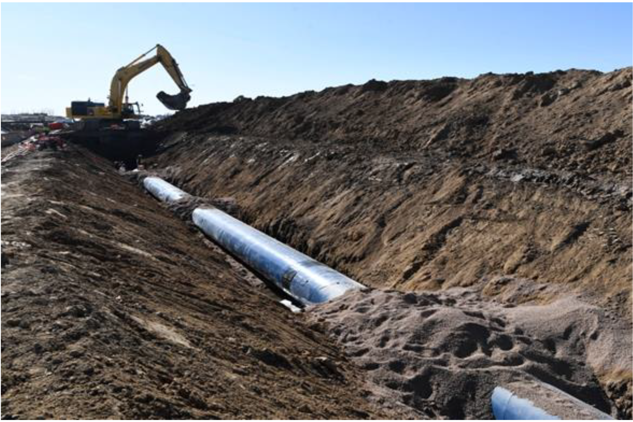
Transmission pipeline systems are the critical infrastructure in the nation’s energy sector that provides economic and safe transportation of large volumes of crude oil, hazardous liquid, or natural gas (NG) over long distances to meet increasing energy demands. It has been predicted that NG demand will be increased by 43% worldwide by 2040 [1]. While some pipelines are built above ground, the majority of pipelines in the U.S. are buried underground per regulations to protect them from damage and to help protect our communities as well. Figure 1 shows a gas transmission pipeline being buried in construction. Because line pipes are made of carbon steels, the steel pipes in underground water or in sour soils are susceptible to external corrosion attack, which poses a big threat to buried pipeline integrity. Based on a statistical analysis of recent significant incidents for crude oil and NG pipelines, Dai et al. [2] showed that external corrosion is a leading failure cause for both oil and gas pipelines. Therefore, corrosion assessment is essential for pipeline design and for pipeline integrity management [3].
In general, unprotected buried steel pipelines are highly susceptible to external corrosion. Without proper corrosion protection, every steel pipeline will eventually deteriorate because metal corrosion weakens pipeline strength and degrades pipeline load-carrying capacity. To prevent pipelines from external corrosion, coating and cathodic protection are required by regulations. Usually, buried pipeline management must cope with other extreme geological conditions, including a range of geohazards, such as ground shaking in seismically active regions, land sliding, ground subsidence and settlement, geological fault displacements, and freeze–thaw displacements [3,4]. This work only considers corrosion effect on the burst strength of buried pipelines subject to internal pressure. For this situation, overburden pressure on buried pipelines can be neglected since it is insignificant in comparison to internal pressure [5,6].
For predicting the burst strength of pressure vessels, numerous empirical, analytical, and numerical models have been developed for defect-free cylinders or pipes subject to internal pressure, as reviewed by Christopher et al. [7] for thick-walled pressure vessels and by Law and Bowie [8] and Zhu and Leis [9] for thin-walled line pipes. In order to consider the material plastic flow effect, Zhu and Leis [10,11] developed an average shear stress yielding theory and obtained the associated Zhu–Leis solution for burst pressure of thin-walled pipelines. Experimental evaluations [9,10] showed that the Zhu–Leis solution provides the most accurate prediction of burst pressure for defect-free, thin-walled pipes. In addition, Zhu [12] evaluated the strength criteria and plastic flow criteria used in pressure vessel design and analysis. The evaluation results showed that the Tresca criterion determines a lower bound result, the von Mises criterion determines an upper bound result, and the Zhu–Leis criterion determines an averaged result.
The pipeline industry began to investigate the threat posed by external corrosion in the late 1960s, and the early experimental data and analytical models were published in the 1970s [13,14,15]. Full-scale burst tests were conducted on pipe segments removed from service, and burst pressure test data were trended as a function of the length and depth of corrosion defects for vintage NG pipeline steels. Two trending functions in the NG-18 equations [14,15] were developed at the Battelle Memorial Institute in the early 1970s for determining fracture failure of steel pipelines containing cracks. Based on the NG-18 equation for collapse-controlled failure, the American Society of Mechanical Engineers (ASME) in cooperation with the oil and gas industry codified an empirical corrosion assessment method in 1984 and published it as ASME B31G [16]. The Modified B31G was published in 1989 and revised in 2009 to reduce the conservatism in B31G.
With advances in steel-making technology, both the strength and toughness of modern pipeline steels have significantly improved, and many high-strength pipeline grades, such as X70 and X80, are being utilized today. Accordingly, over the past few decades, many improved corrosion assessment models [17] have been developed to improve the management of high-strength pipelines. Among them, the ultimate tensile stress (UTS)-based models can determine improved burst pressure of corroded pipelines and have been accepted by the British Standard BS 7910 [18] and American Standard API 579 [19] for a general fitness-for-service (FFS) assessment of cylindrical pressure vessels, including pipelines. However, ASME B31G and Mod B31G remain in use today in the pipeline industry, even though these models are known to be generally (overly) conservative.
In order to obtain a commonly accepted corrosion assessment model, both academic and industry researchers continue to make efforts to improve assessment methods for buried pipelines. Recently, Zhu [20,21] compared available corrosion assessment methods for metal-loss or corrosion defects in pipelines and discussed real-world challenges facing the oil and gas industry. Zhou and Huang [22] assessed the errors of existing corrosion prediction models. Zhu [23] discussed finite element analysis (FEA) approaches used to predict the burst pressure of pipelines with corrosion defects. Leis et al. [24] presented FEA numerical results that minimized the uncertainty in ASME B31G corrosion assessment model. Heggab et al. [25] performed an FEA numerical sensitivity study of burst pressure for corroded pipes. Oh et al. [26] proposed a new FEA burst model for defect-free pipelines. Bhardwaj et al. [27] developed two burst strength prediction models for X100 and X120 ultra-high-strength corroded pipes. Amaya-Gomez et al. [28] assessed the reliability of various available corrosion models. Bhardwaj et al. [29] quantified the uncertainty of existing burst pressure models for corroded pipelines. Most recently, Cai et al. [30] developed data-driven methods for predicting the burst strength of corroded pipelines. Li et al. [31] reviewed 71 intelligent models for predicting burst pressure, corrosion growth rate, remaining thickness, and corrosion depth for managing corroded pipelines using different methods, including fuzzy mathematics, artificial neural network (ANN), chaos theory, and support vector machine learning method.
In 2021, the U.S. Department of Energy (DOE) sponsored a multiple-year Laboratory Directed Research and Development (LDRD) program at the Savannah River National Laboratory (SRNL) to develop an advanced plasticity theory and a machine learning technology for determining the burst strength of high-pressure vessels with and without corrosion defects. Fruitful results have been achieved from this LDRD program, including a new strength theory and its application to determine burst strength of thick-walled pressure vessels [32], an innovative machine learning model of burst strength for defect-free pipes [33,34], an advanced FEA model for predicting the burst strength of thin- and thick-walled pressure vessels [35], a progress review of corrosion assessment model development for pipelines [36], and three new corrosion assessment models for predicting the remaining strength of thick-walled pipelines [37]. This work aims to review these recent advances in corrosion assessment models for predicting the remaining burst strength of corroded thin- and thick-walled pipelines. In addition, a brief review of burst pressure prediction models is also given first to defect-free pipes and then to corroded pipes. For a better understanding of corrosion model development, corrosion assessment models are categorized into four generations and then evaluated with full-scale burst test data. Finally, major technical challenges and gaps are discussed for further study.
2. Burst Pressure Models for Defect-Free Pipes
Burst pressure prediction for defect-free pipes is the basis for developing corrosion models for assessing the remaining strength of pipelines containing corrosion or metal-loss defects [21]. The reference stress embedded in a corrosion assessment model is defined by the burst pressure of defect-free pipes. This section briefly reviews the strength models and the flow models of burst pressure for thin-walled pipes, the new strength theories for thick-walled pipes, an advanced numerical model, and the machine learning models for both thin- and thick-walled pipes.
2.1. Strength Models for Thin-Walled Pipes
For a large-diameter, thin-walled, defect-free pipe, four strength-theory-based models [12] have been obtained for predicting burst pressure in terms of the UTS and the Tresca, von Mises, Zhu–Leis, and the flow stress criterion [13]:
- (1).
- Tresca strength solution:
- (2).
- von Mises strength solution:
- (3).
- Zhu–Leis strength solution:
- (4).
- Flow stress-based failure solution:
To evaluate the accuracy of the strength models of burst pressure in Equations (1)–(4), reference [12] compared the experimental data of burst pressure for more than 100 full-scale tests for thin-walled pipes made of carbon steel with the predictions from the four strength criteria. The comparison showed that (1) the von Mises strength criterion overestimates burst pressure for all steels, (2) the Zhu–Leis strength criterion is acceptable for high-strength steels but overestimates burst pressure for low-strength steels, (3) the Tresca strength criterion adequately predicts burst pressure for intermediate-strength steels, and (4) the flow stress criterion predicts the most conservative results for all steels. Among the four strength criteria, only the flow stress criterion considers the strain-hardening effect on burst pressure. As such, a flow theory of plasticity was recommended [12] for developing more accurate burst pressure solutions in terms of the two material properties of UTS and YS.
2.2. Flow Models for Thin-Walled Pipes
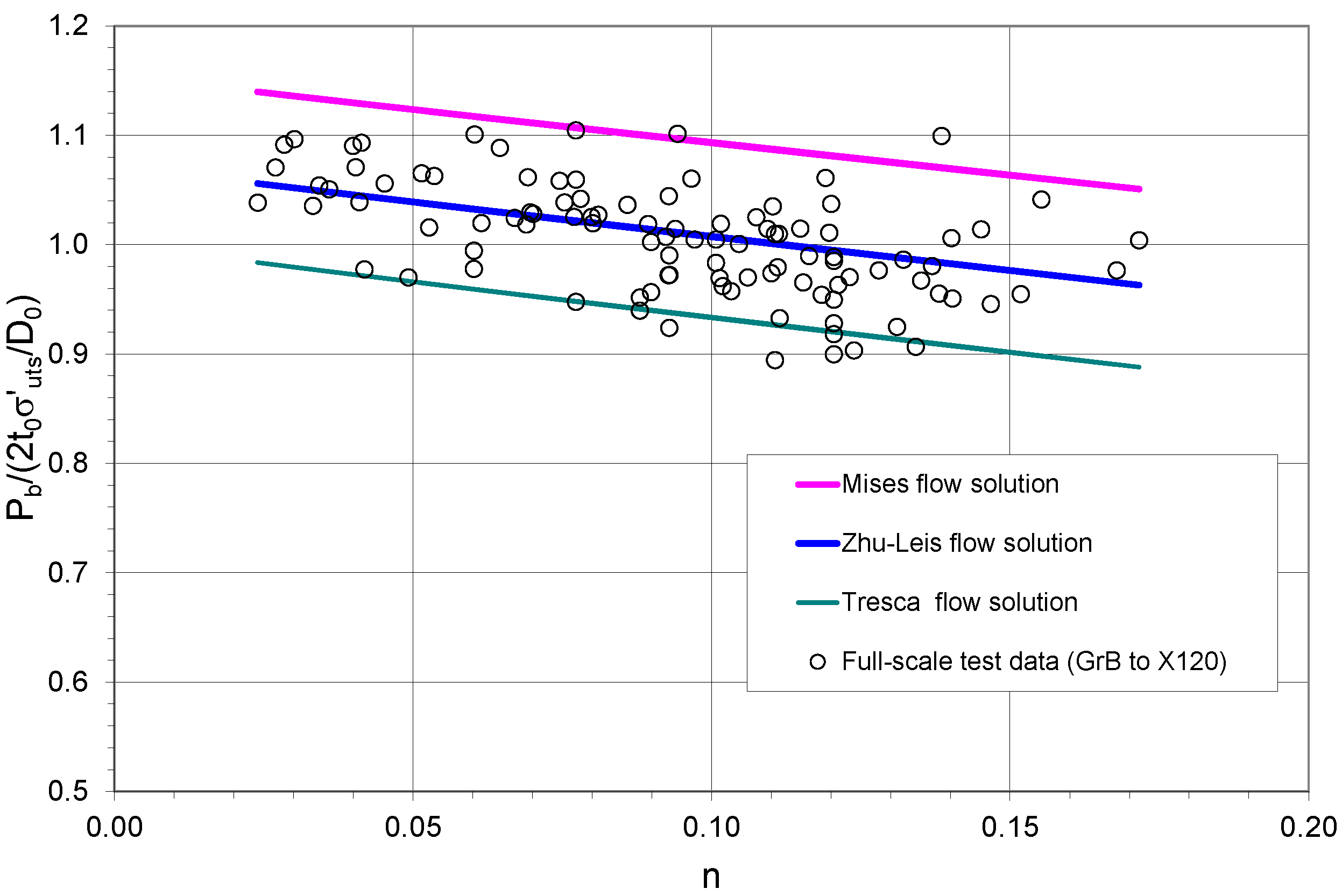
The Tresca theory and the von Mises theory are two classical theories of plasticity that have often been used to describe the nonlinear plastic deformation in a metallic material during loading. These theories can determine two bound solutions for burst pressure of a defect-free pipe. To define more accurate burst failure, Zhu and Leis [10,11] introduced a new concept of “average shear stress” and developed the average shear stress flow theory that is simply referred to as Zhu–Leis flow theory. For a power-law hardening material, this new flow theory determines a new flow solution for burst pressure. As such, these three flow theories determine the Tresca, Zhu–Leis, and von Mises flow solutions of burst pressure for defect-free thin-walled pipes:
where n is the strain-hardening exponent and is usually measured from a tensile test or estimated from the yield-to-tensile-strength (Y/T) ratio [38].
Figure 2 compares the experimental data relating to burst pressure from more than 100 full-scale best tests with the Tresca flow solution in Equation (5), the Zhu–Leis flow solution in Equation (6), and the von Mises flow solution in Equation (7). In this figure, all points denote experimental data, and all lines denote burst pressure predictions. Experimental data details were described in reference [10]. All pipe materials used in the burst tests were ductile, low-carbon steels with a wide-ranging strain-hardening exponent n from 0.02 to 0.18 that covers low-to-high-strength pipeline steels from Grade B to X120. From the figure, it can be observed that (1) both test data and predictions of burst pressure are functions of the strain-hardening exponent in a similar trend, (2) the von Mises flow solution provides an upper bound prediction, (3) the Tresca flow solution provides a lower bound prediction, and (4) the Zhu–Leis flow solution provides the best prediction that matches well with the burst data on average. Thus, these experimental data validate the Zhu–Leis flow theory and the associated flow solution for burst pressure of defect-free thin-walled pipes.
Using other full-scale burst test databases, Zimmermann et al. [39], Zhou and Huang [40], Bony et al. [41], and Seghier et al. [42] all confirmed that the average shear stress yield criterion is the best plastic yield criterion and that the Zhu–Leis flow solution is the most accurate burst pressure prediction for thin-walled pipes. The same conclusions were recently verified by Bhardwaj et al. [27] for X100 to X120 ultra-high-strength pipeline steels and by Amaya-Gomez et al. [28] and Bhardwaj et al. [29] for a wide range of pipeline grades from Grade B to X100. Thus, the Zhu–Leis flow theory [10] fills in the technical gap between the classical Tresca and von Mises flow theories and determines a more accurate burst pressure solution.
2.3. Burst Pressure Models for Thick-Walled Pipes
The burst pressure models discussed above are based on the thin-shell theory, and, thus, they are applicable only to thin-walled pipes with D/t ≥ 20. In practice, there are many thick-walled line pipes with a wall thickness larger than 20 mm [43], leading to D/t < 20. In this case, the thin-shell theory becomes invalid, and the thick-shell theory should be applied. For thick-walled pipes with D/t < 20, both axial and hoop stresses are not constant anymore through the wall thickness, and the wall thickness becomes an important factor for pipeline design and integrity management. Note that D/t = 20 is an engineering definition to distinguish thin-walled and thick-walled pipes.
In order to obtain a burst pressure solution for thick-walled pipes, Zhu et al. [32] recently proposed a two-parameter-based flow stress and developed a new strength theory that can predict the plastic collapse of a pressure vessel. On this basis, the following burst pressure solution was obtained for defect-free thick-walled pipes:
where C is a constant that is related to the yield criterion:
where D0 (Di) is the outside (inside) diameter. Equation (10) is the burst pressure solution for thick-walled pipes corresponding to the Tresca, von Mises, and Zhu–Leis criteria.
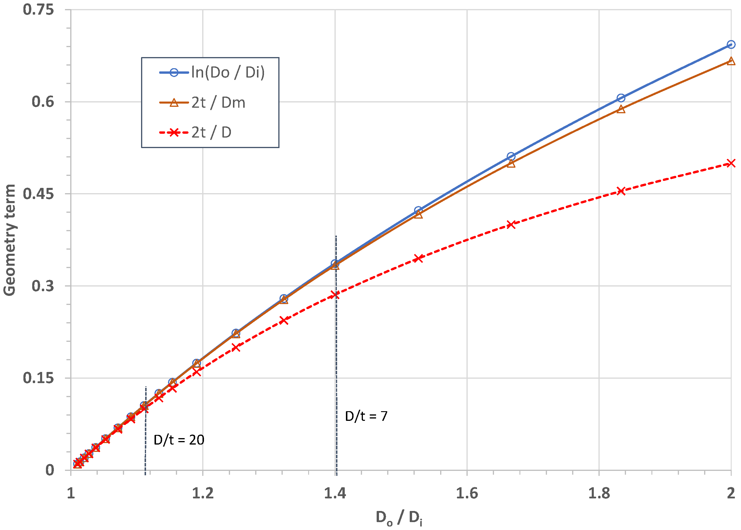
Comparison of the burst solution in Equation (8) with those in Equations (5)–(7) shows that the reference stresses are the same, but the geometry terms are different. For the thin-walled solution, the geometry term is 2t/Dm if the mean diameter (MD) Dm = D-t is used or 2t/D if the outside diameter (OD) is used. For the thick-walled solution, the geometry term is ln(Do/Di). Figure 3 compares these three geometry terms for different diameter ratios. As evident in this figure, the geometry term 2t/Dm is very close to ln(Do/Di) when the Do/Di ratio is less than 1.4 (or D/t ≥ 7) and where the differences are insignificant and less than 1.0%. For thin-walled pipes with D/t ≥ 20 (or Do/Di ≤ 1.111), the differences are less than 0.1%. This observation suggests that the mean diameter Dm should be used in the thin-shell theory for predicting more accurate burst pressure for D/t ≥ 20. In contrast, if the outside diameter is used, the difference between the two geometry terms 2t/D and ln(Do/Di) becomes very large for a diameter ratio larger than 1.2. The difference reaches 5.1% at D/t = 20. As such, the outside diameter is not recommended for use in pipeline design and integrity assessment.
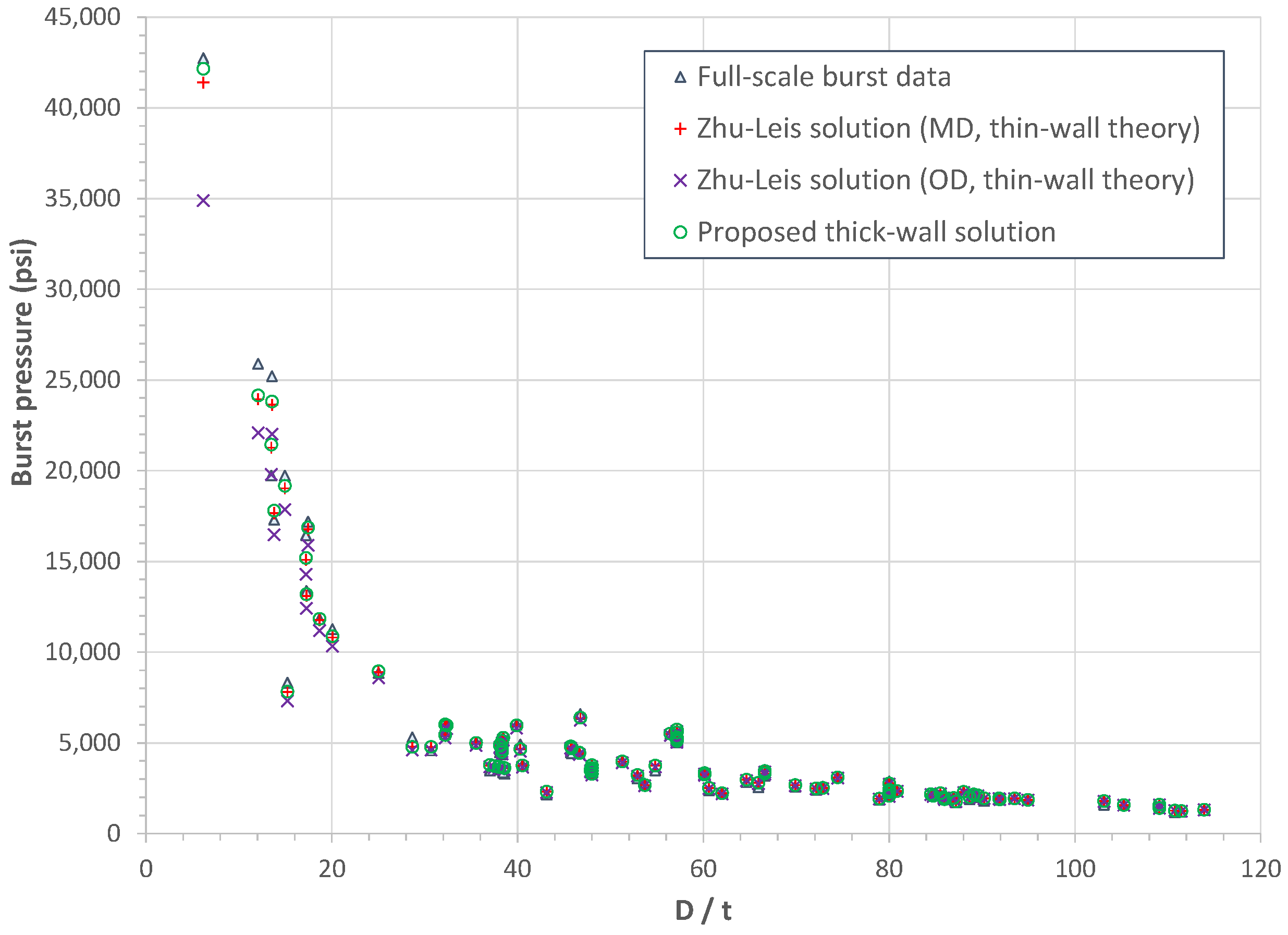
Figure 4 compares the Zhu–Leis burst pressure solutions from Equations (6) and (8) with the full-scale burst data (as shown in Figure 2 with limited burst data for thick-walled pipes) as a function of . From this figure, it can be observed that:
- The newly proposed Zhu–Leis solution for thick walls in Equation (8) is very accurate and closely matches the burst pressure data for all pipes, from thin to thick walled;
- For thin-walled pipes with , the Zhu–Leis solution from the thin-shell theory is very accurate and close to that from the thick-shell theory;
- For intermediate-to-thick-walled pipes with , the MD-based Zhu–Leis solution for thin-walled pipes is nearly identical to that for thick-walled pipes;
- In contrast, the OD-based Zhu–Leis solutions for thin-walled pipes are significantly lower than those for the thick-walled pipes when D/t < 10. As a result, the MD-based rather than OD-based Zhu–Leis solution should be used generally in the thin-walled burst solution.
2.4. Advanced Numerical Model of Burst Pressure
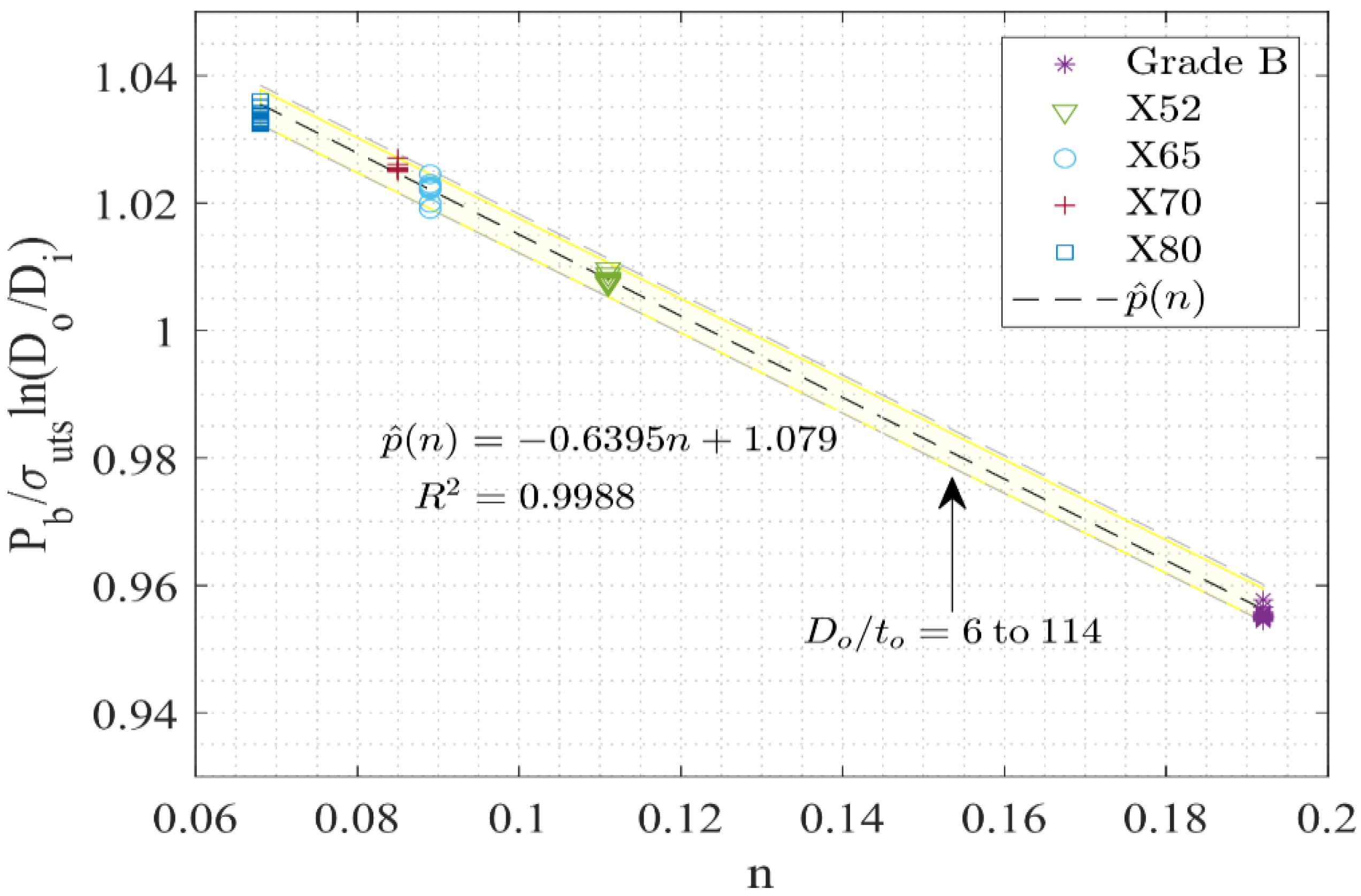
Johnson et al. [35] performed a comprehensive FEA parametric study of burst pressure using Abaqus Python script technology that rapidly iterated over 60 different FEA cases to cover a wide range of pipeline grades from Grade B to X80 and a large range of pipeline geometries from D/t = 6 to 120. For both thin- and thick-walled pipes, it demonstrated that the pipe burst failure can be accurately defined in the FEA calculations when the von Mises stress at the middle wall thickness (or the mean diameter) reaches the critical von Mises stress of the pipeline steel [44]. Figure 5 shows the numerical data of the burst pressure that was normalized by the thick-walled Tresca strength solution as a function of the strain-hardening exponent n for all 60 FEA cases. It was found that the FEA data for the normalized burst pressure can be well fitted as a linear function of n with a very high goodness-of-fit measure of R2 = 0.9988.
Based on the FEA results of burst pressure and the linear fit function, a linear regression model of burst pressure for both thin- and thick-walled pipes was thus obtained as a function of Do/Di, UTS, and n in the simple form of:
2.5. Machine Learning Models of Burst Pressure
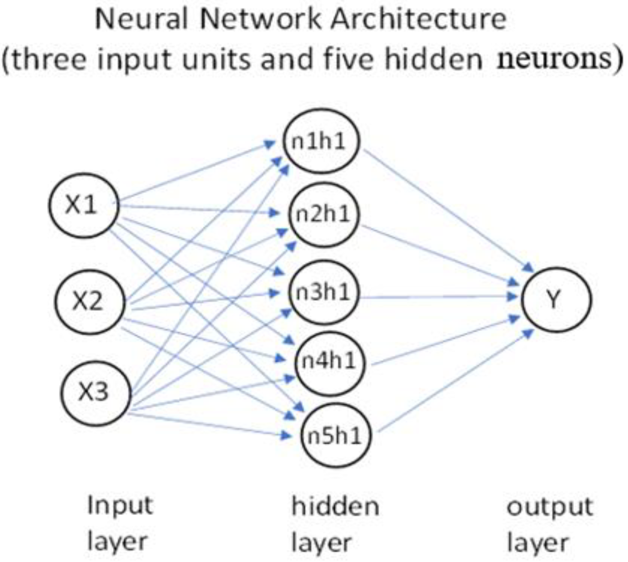
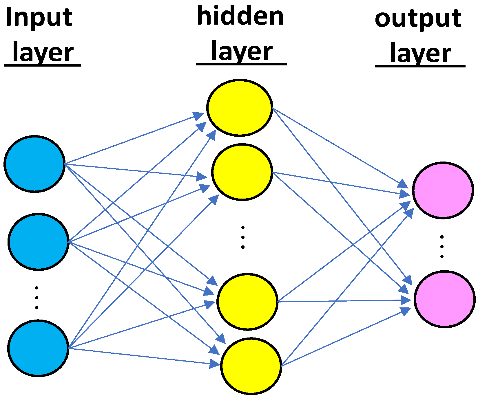
Recently, Zhu et al. [33,34] applied machine learning technology to model the burst strength of defect-free pipes for a wide range of D/t ratios and steel grades. Using the full-scale burst database shown in Figure 2, three ANN architectures were created, and three ANN models of burst pressure were determined. ANN model 1 has one input variable and one hidden layer, ANN model 2 has three input variables and one hidden layer, and ANN model 3 has three input variables and two hidden layers. All three ANN models have one output variable. The architecture of ANN model 2 is shown in Figure 6, where the three input variables are X1 = n, X2 = UTS, and X3 = D/t, and the output variable Y = Pb. For each ANN model, two activation functions (Sigmoid and linear functions) were used to connect neurons in different layers with weights and bias at each unknown neuron. The activation functions coupled with specific algorithms were used to train and learn from the training dataset until the model performance is satisfied in comparison to the test dataset. The ANN models can be used to predict burst pressure for both thin- and thick-walled pipes without particular consideration of the wall-thickness effect.
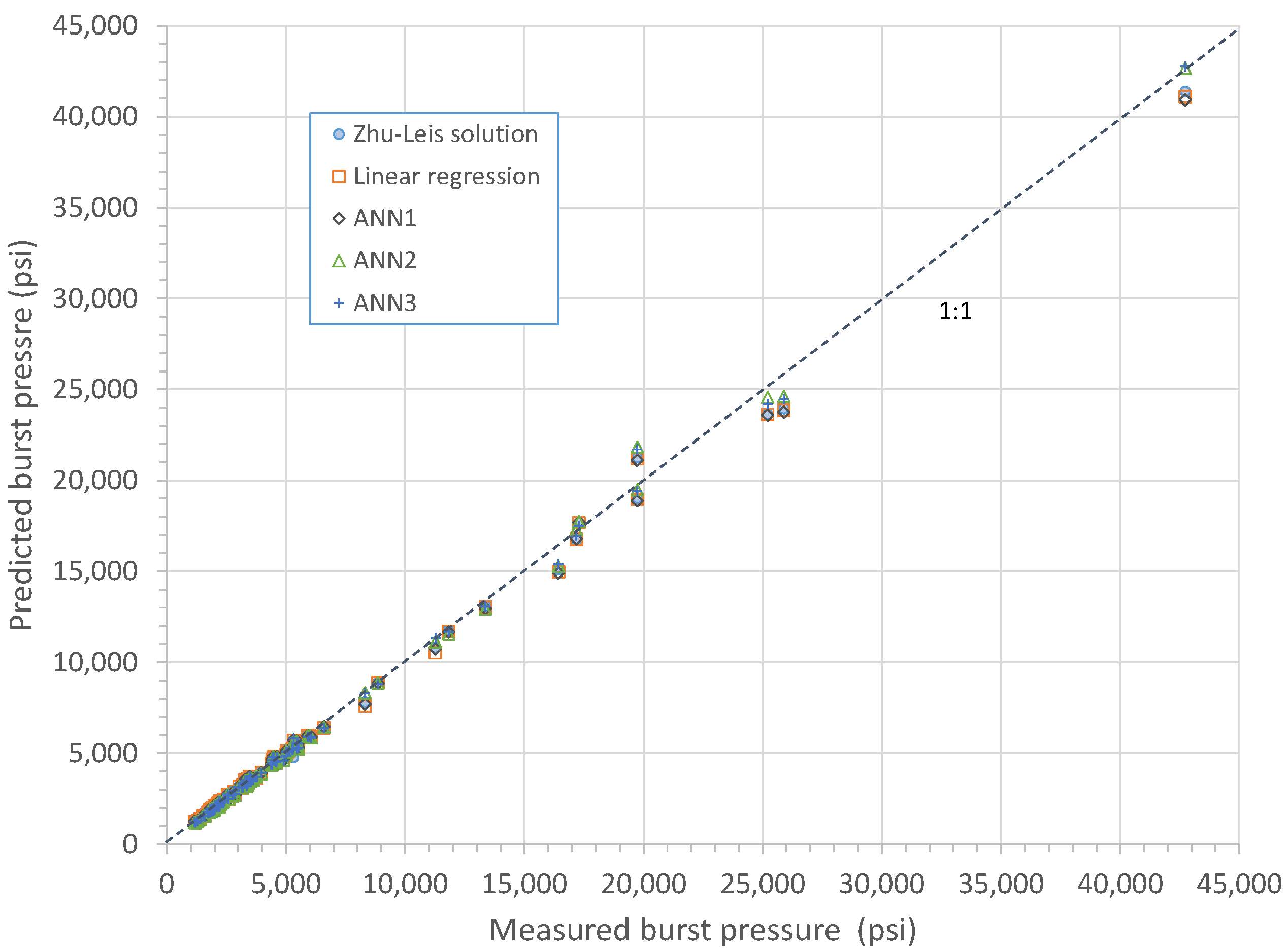
Figure 7 compares the model predictions with the experimental burst data for the full-scale tests, as shown in Figure 2, where the model predictions include those predicted by the three ANN models, the linear regression, and the Zhu–Leis solution for thick-walled pipes. As evident in this figure, all model predictions were nearly identical to the burst data when the measured burst pressure is less than 15 ksi (103.42 MPa). Otherwise, some deviations were observed, and ANN model 2 and model 3 predicted the most accurate burst pressure. Due to the simple architecture, ANN model 2 is recommended as the best machine learning model for predicting the burst pressure of defect-free thin- and thick-walled line pipes.
3. Corrosion Assessment Models
Corrosion defects in aged pipelines may have complex features in terms of size, shape, location, and orientation. This study only considers a single axially oriented, isolated corrosion defect in a pipeline subject to internal pressure. Multiple corrosion defects, corrosion interaction, and other anomalies are not considered.
A general expression of burst pressure for a single corrosion defect in thin-walled pipelines can be written [19,21] as:
where SR is a reference stress, 2t/D is the thin-walled pipe geometry term, and f is a defect geometry term that is defined as a function of defect geometry (depth d, length L, and width W). In many cases, defect width has an insignificant effect, and f can be simplified as f (d/t, L/√(Dt)). Without a defect, Equation (11) reduces to that of a defect-free pipe, and, thus, SR is equal to the burst strength of a defect-free pipe. Note that Equation (11) is consistent with the notation used in API 579 [14] for the level 1 corrosion criterion.
Pb = SR × 2t/D × f (defect geometry)
Based on different definitions of the reference stress, available corrosion assessment models can be categorized into four generations, as discussed next.
3.1. The First-Generation Models (1960s–1980s)
The first-generation models for assessing the remaining strength of corroded pipes were developed empirically in the 1960s to 1980s with the reference stress SR = flow stress.
3.1.1. ASME B31G
From full-scale test data obtained in the early 1970s for pipeline steels up to X65, Maxey et al. [14,15] developed several semi-empirical equations (i.e., NG-18 equations) for predicting the burst pressure of line pipes with cracks. On this basis, a corrosion assessment model was codified by ASME in 1984 and published as B31G. For an actual short defect, the corrosion area was assumed to be parabolic in shape with a curved bottom, and the burst pressure of the corroded pipeline was obtained as:
where the defect depth is limited within 80% of the wall thickness or d/t ≤ 0.8.
For a long corrosion defect, the corrosion area was simplified as a rectangle with a flat bottom, and Equation (12) becomes:
In both equations above, the flow stress , where SMYS is the specified minimum yield stress defined in API 5L [45], and M is a Folia’s bulging factor [46]:
Note that ASME B31G was calibrated for vintage pipeline grades up to X65, and so it may be inadequate to use for modern pipeline steels such as X80 or X100.
3.1.2. Mod B31G (0.85 dL)
3.1.3. RSTRENG (Effective Area Model)
A real corrosion defect has a river-bottom profile. Kiefner and Vieth [48] proposed an effective area method to improve the remaining strength prediction:
where the flow stress σf and the bulging factor M are the same as in Mod B31G, Ad denotes the effective area of a complex corrosion defect profile, and A0 = tL is the axial cross-section area. This model determines a more accurate corroded area using the discrete approach and then a more accurate burst pressure of a real corrosion defect. A personal computer code called RSTRENG [48] was developed for iterating more accurate burst pressure for corroded pipes. This effective area model was adopted in the level 2 procedure of ASME B31G [16] and API 579 [19]. Recently, Yan et al. [51] improved the RSTRENG using a more efficient effective area method for corrosion assessment.
For a machined rectangular defect with a uniform depth, Equation (17) becomes:
For a long corrosion defect, 1/M approaches zero, and Equation (18) reduces to Equation (13). In 1992, Richie and Last [52] adapted Equation (18) as a corrosion defect acceptance criterion (i.e., Shell-92 model) with the flow stress .
3.1.4. CSA Z662
From the Shell-92 model, the Canadian Standards Association (CSA) developed a corrosion assessment code—CSA Z662 [53]—for predicting burst pressure:
where dave is the averaged defect depth, the bulging factor M is the same as Equation (16), and the flow stress is defined as:
3.1.5. Comparison of the First-Generation Models
Reference [21] compared the first-generation models discussed above for a flat defect with a depth of d/t = 0.5 in two lower pipeline steels, X52 and Grade B.
For the X52 steel, the comparison showed that the Modified B31G predicts the highest burst pressure for all defect lengths, CSA Z662 and Shell-92 are identical with predictions slightly lower than the RSTRENG results, and ASME B31G predicts a comparable result to Modified B31G for a short defect but the lowest result for a long defect.
For the Grade B steel, the comparison showed that the Shell-92 model predicts the highest results of burst pressure over the given defect length, and, following in order, are the Mod B31G, RSTRENG, and CSA Z662 models. The ASME B31G model may predict a comparable result to RSTRENG for a short defect but the lowest result for a long defect.
3.2. The Second-Generation Models (1990s–2000s)
The second-generation models for predicting the remaining strength of corroded thin-walled pipelines were developed numerically from the FEA simulations in the 1990s to 2000s with SR = UTS. All these models did not consider the defect width effect.
3.2.1. LPC Model
Based on a large number of elastic-plastic FEA results and burst test data for X65 corroded pipelines, a line pipe corrosion (LPC) model was developed at British Gas in 1995 [54,55] for determining the burst pressure of corroded thin-walled pipes:
where D-t is the mean diameter, and Q is a curve-fit bulging factor from the FEA results:
3.2.2. PCORRC Model
In parallel to the LPC development, a pipeline corrosion criterion (PCORRC) was developed from FEA calculations at Battelle in 1997 [57,58]:
where the outside diameter D is used rather than the mean diameter used in the LPC model. The difference between t/D and t/(D-t) exists for intermediate-walled pipes, as shown in Figure 3.
For a very long defect in thin-walled pipes, Equation (23) reduces to a simple equation:
In this case, Equation (21) reduces to Equation (24) with D-t used in the place of D. If a defect is absent, Equation (24) reduces to Equation (1) or the Tresca strength solution for defect-free pipes. This implies that both the LPC and PCORRC models have the basis of the Tresca criterion with one single material parameter.
3.2.3. Choi Limit Load
In 2003, Choi et al. [59] conducted a set of full-scale tests on machined metal-loss defects for X65 pipeline steel and performed 3D elastic-plastic FEA calculations on the test defects where all axial defects were assumed to be elliptically curved. By trending the FEA outcomes, they obtained the limit load as:
where Di is the inside diameter, R is the mean radius, and C0, C1, C2, C3, and C4 are functions of d/t. Lacking a defect, Equation (25) reduces to Pb = 0.9σuts × 2t/Di for defect-free pipes. As a result, the limit load in Equation (25) may be conservative for thin-walled pipes.
3.2.4. Recalibrated PCORRC Model
Based on full-scale test data and a set of 3D FEA calculations for X70 corroded pipes, Yeom et al. [60] in 2015 recalibrated the PCORRC model as follows:
Lacking a defect, Equation (26) reduces to Pb = 0.9σuts × (2t/D) for defect-free pipes. This model may be also conservative.
In the mid-2000s, the U.S. DOT PHMSA Pipeline Office sponsored a large corrosion program [61] to evaluate the first- and second-generation corrosion models using a large experimental database that contains 313 burst tests, including full-scale vessel tests and ring expansion tests for real and machined defects for pipeline grades from Grade A25 to X100. Useful guides were then provided for pipeline operators to use the corrosion models in pipeline integrity assessment.
3.2.5. Comparison of the Second-Generation Models
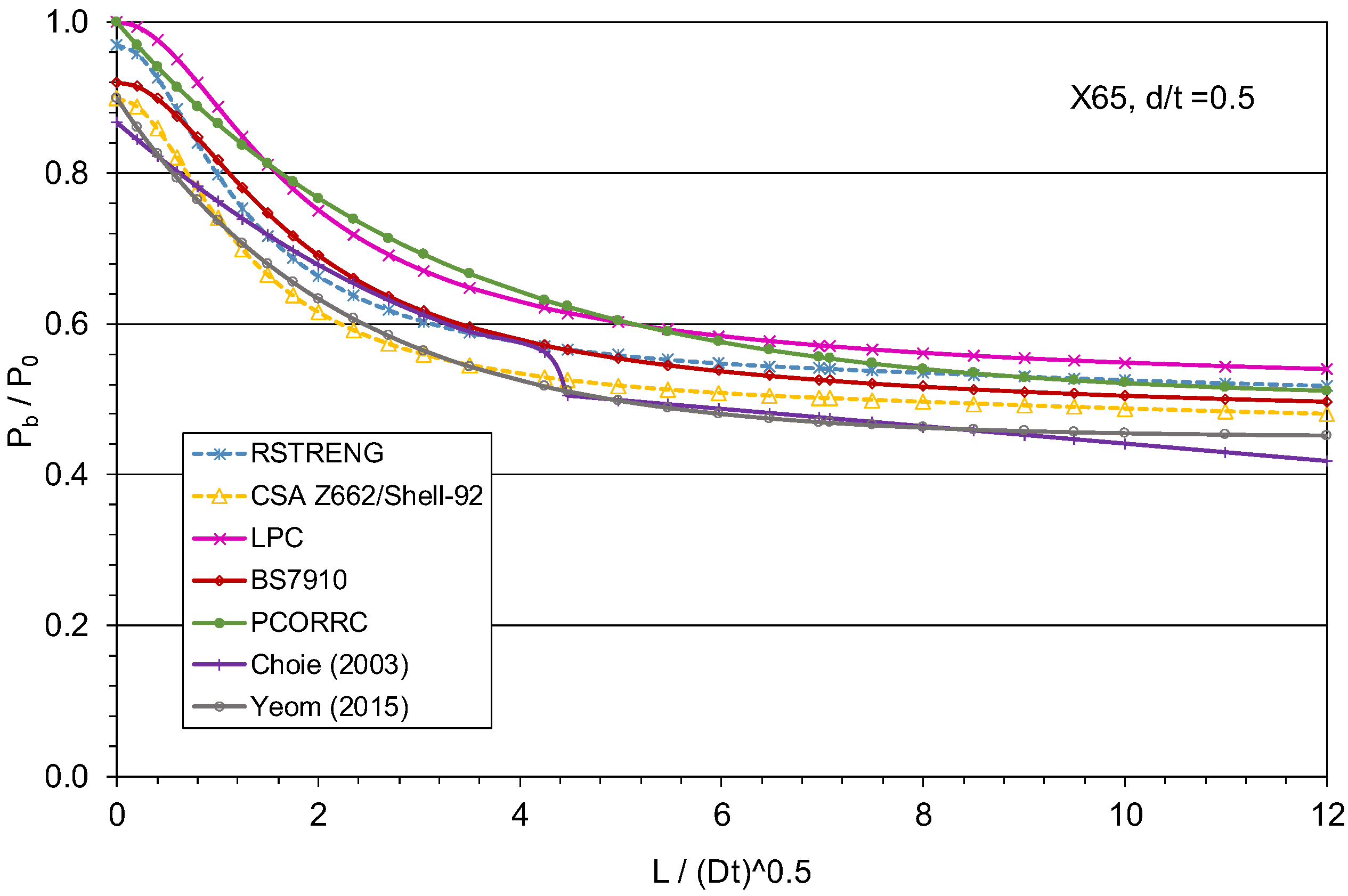
Figure 8 compares the second-generation models discussed above for a fixed, uniform defect depth of d/t = 0.5 in a pipeline of intermediate-strength steel, X65, where the material properties are assumed to be the SMYS and SMTS of X65. In this figure, six second-generation models are included: LPC (DNV), BS 7910, PCORRC, limit load by Choi (2003), and Reformulated PCORRC by Yeom (2015). For comparison, RSTRENG and CSA Z662 are also included in Figure 8. This figure shows that (1) LPC and PCORRC predict comparable results, (2) BS 7910 and RSTRENG predict similar results that are lower than the LPC predictions, (3) CSA Z662 and the Yeom (2015) model predict comparable results that are lower than RSTRENG predictions, and (4) the Choi (2003) and Yeom (2015) models are comparable for short defects and become almost identical, becoming the lower bound for long corrosion defects.
3.3. The Third-Generation Models (2000 to 2020)
The third-generation models consider the material strain-hardening effect, and the reference stress is a function of UTS and n, or SR = f (UTS, n). Recently, Zhu [15] detailed seven third-generation models. Four of them are accurate and discussed in this section.
3.3.1. von Mises Flow Model Coupled with Reformulated PCORRC
In 2013, Ma et al. [62] utilized the von Mises flow strength in Equation (7) as the reference stress SR, which was coupled with the geometry term of PCORRC. After recalibration with their FEA results of burst pressure for a variety of machined defects in X70 and X80 pipes, these authors reformulated PCORRC model as:
Comparison of Equations (27) and (23) shows the geometry term embedded in Equation (27) is quite different from that used in the original PCORRC model.
3.3.2. Mod PCORRC Model Coupled with Zhu–Leis Flow Solution
In 2018, Zhu [63] modified the PCORRC model with use of the Zhu–Leis flow solution in Equation (6) as the reference stress. The defect geometry function was assumed to be unchanged for corrosion defects. The Mod PCORRC model is expressed as:
3.3.3. Mod LPC Model Coupled with Zhu–Leis Flow Solution
In 2021, Zhu [21] proposed a modified LPC model using the Zhu–Leis flow solution as the reference stress. The defect geometry function was also assumed to be unchanged for corrosion defects with flat bottoms. The Mod LPC model is expressed as:
3.3.4. A Polynomial Corrosion Model
In 2015, Zhu [23] developed a new corrosion model. The reference stress was defined from the Zhu–Leis solution in Equation (6) for defect-free pipes, and the defect geometry term determined from FEA results contains a polynomial. This polynomial corrosion model is expressed as:
where g is a polynomial function with a degree of 2:
3.3.5. Comparison of the Third-Generation Models
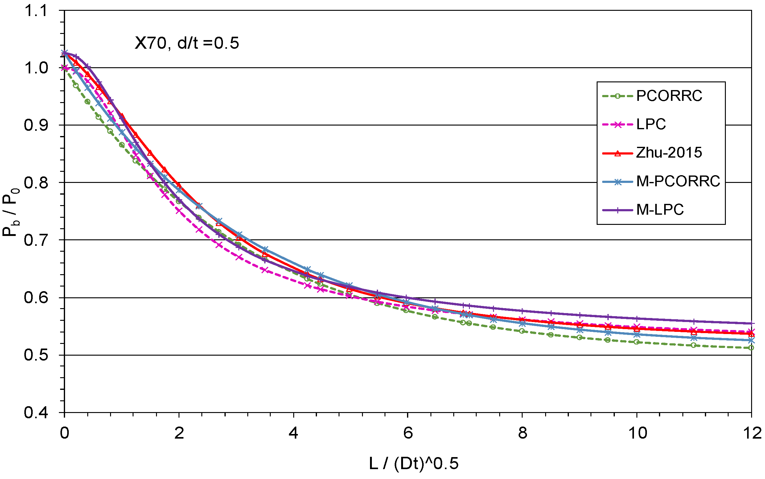
Figure 9 compares Mod LPC with LPC and Mod PCORRC with PCORRC. The Zhu 2015 model is also included in this figure. It can be observed that (1) Mod LPC is shifted up from the LPC by a factor of 1.03, (2) Mod PCORRC is shifted up from the PCORRC by the same factor of 1.03, and (3) the two modified models are close to the Zhu 2015 model. Therefore, all five corrosion models predict comparable burst pressures.
3.4. Validation of Corrosion Assessment Models
3.4.1. Experimental Validation of the Third-Generation Models
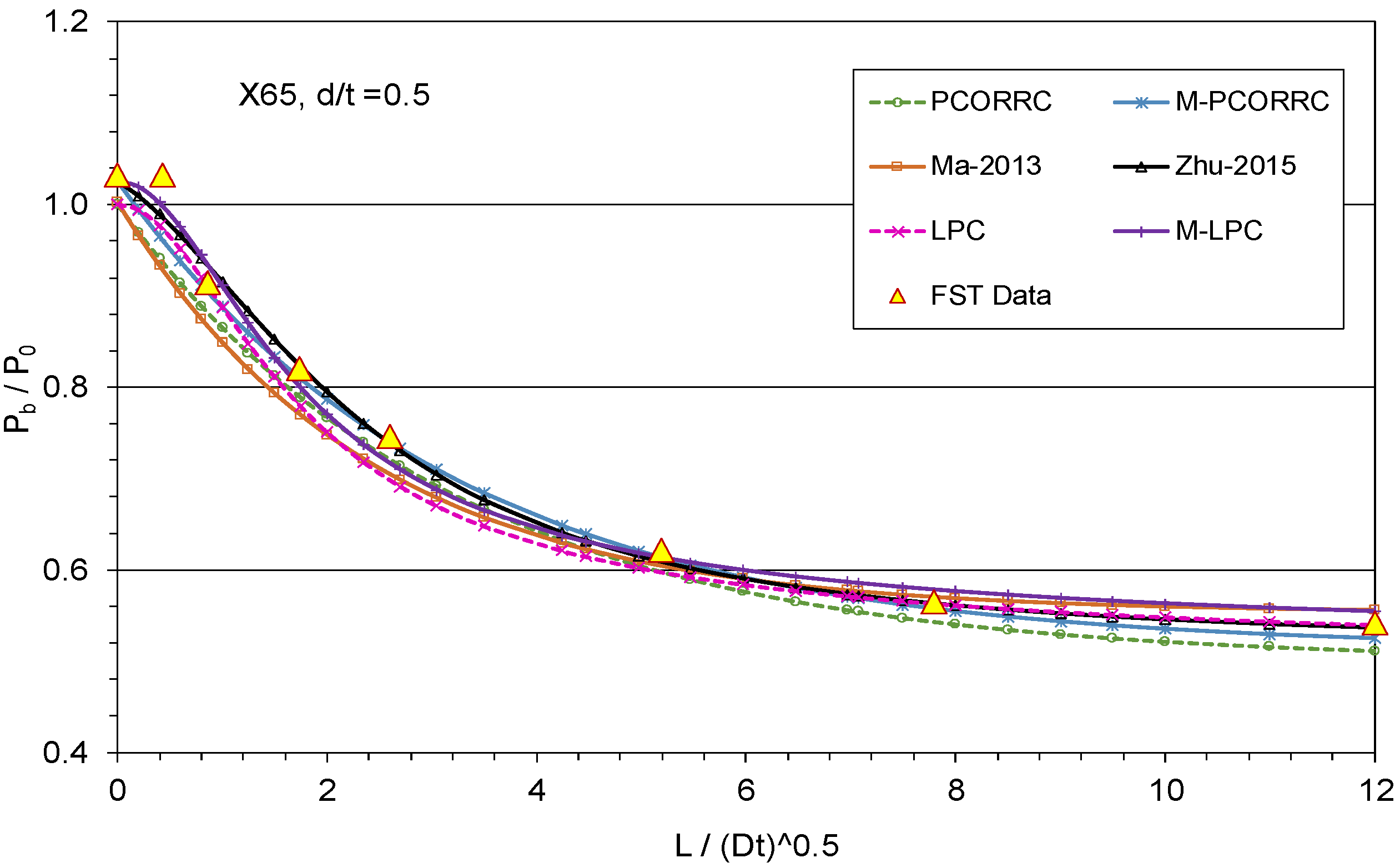
Kim et al. [64] conducted a set of full-scale burst tests for machined metal-loss defects and obtained reliable burst pressure data for X65 pipeline steel. The burst pressure data were reported for machined metal-loss defects with a fixed, uniform depth of d/t = 0.5 and six defect lengths of L = 50, 100, 200, 300, 600, and 900 mm. The pipe diameter was 762 mm (30 in) and the wall thickness was 17.5 mm (0.69 in). The actual YS and UTS of the X65 pipe were 495 MPa (71.8 ksi) and 565 MPa (81.9 ksi), respectively.
Figure 10 compares the four third-generation models (i.e., Ma 2013, Mod PCORRC, Mod LPC, and Zhu 2015) and the two second-generation models (i.e., PCORRC and LPC) with the experimental burst data obtained by Kim et al. [64]. All these six models predict comparable results that closely match the burst test data. However, further observation shows that (1) the PCORRC is slightly conservative for all defects, (2) the LPC is conservative for short defects, (3) the Ma 2013 model is conservative for short defects and slightly non-conservative for long defects, (4) the Mod LPC is accurate for short defects and slightly non-conservative for long defects, and (5) the Zhu 2015 and Mod PCORRC models are nearly identical to each other and the most accurate in comparison to the full-scale test data.
3.4.2. Experimental Validation of Mod PCORRC Model
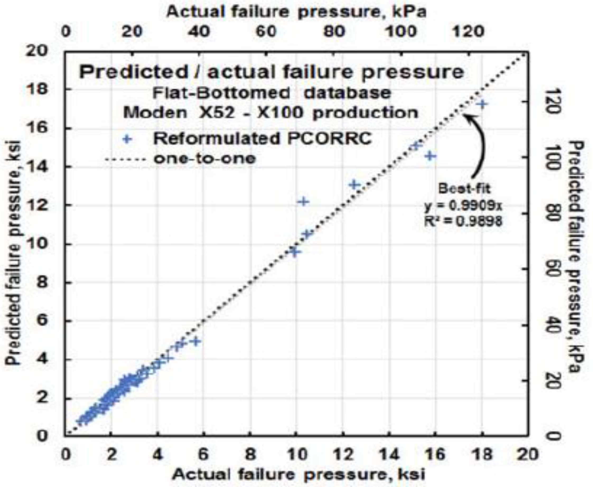
More recently, Leis [65] assessed the reference stress, the geometry term of the PCORRC model, and the reformulated PCORRC using full-scale burst data for machined defects with flat bottoms for a wide range of pipeline grades ranging from X52 to X100. Figure 11 compares the predictions from the Mod PCORRC model in Equation (28) with the actual failure pressure for the machined defects. As evident in this figure, the predictions agree well with the actual data with a very high best-fitting correlation factor of 0.991 between the model predictions and the actual burst pressure data.
Similarly, Leis [65] also evaluated the Mod PCORRC model using the calibration database of ASME B31G and Mod B31G for a set of complex actual corrosion defects that have irregular river-bottom shapes. The comparison also showed a good agreement between the predicted outcomes and the actual failure pressure with a best-fitting correlation factor of 0.922. In contrast to this, the corresponding best-fitting correlation factor was 0.617 and 0.698 for B31G and Mod B31G, respectively. Thus, the full-scale burst data validated the accuracy of the proposed Mod PCORRC model in Equation (28). This model is adequate to use for predicting more accurate burst pressure for thin-walled pipelines with corrosion or metal-loss defects.
4. Recent Development of Corrosion Models (Fourth Generation)
Since 2021, the U.S. DOE SRNL has started to sponsor the development of a fourth-generation corrosion model to consider both the pipe wall-thickness effect and the material strain-hardening effect on the remaining strength of corroded pipes. Similar to Equation (11), a general expression of burst pressure for corroded, thick-walled pipes can be written as:
where the reference stress SR is the burst strength for defect-free pipes in terms of the Zhu–Leis flow theory, that is, . The logarithmic function ln(Do/Di) is the pipe geometry term for thick-walled pipelines, and f is the defect geometry term.
4.1. Thick-Wall Burst Pressure Solutions
For corrosion defects in thick-walled pipes, it is assumed that the defect geometry function of a corrosion model for thick-walled pipes is approximately the same as that for thin-walled pipes, and the defect width effect is not considered. As such, Zhu et al. [37] adapted the three third-generation corrosion models discussed in Section 3.3, including the Mod PCORRC model in Equation (28), Mod LPC model in Equation (29), and the polynomial model in Equation (30), for thin-walled pipes, and proposed three new corrosion models for thick-walled pipes as follows:
These corrosion models for thick-walled pipes have an improved, higher accuracy compared to that for thin-walled pipes, as demonstrated next.
4.2. Experimental Validation of Thick-Wall Models
A large burst test database containing 80 full-scale burst test data [65] was utilized here to evaluate and validate the proposed corrosion models for thick-walled pipes. The full-scale burst tests involved machined defect features with flat bottoms for pipeline steel grades of X46, X52, X60, X65, X70, X80, and X100. The tested pipes had diameters ranging from small (8.63 in or 219 mm) to large (52 in or 1321 mm) and wall thicknesses ranging from thin wall (0.233 in or 5.92 mm) to thick wall (1.0 in or 25.4 mm). As a result, the D/t ratios ranged from 8.6 (thick-walled pipe) to 81.8 (thin-walled pipe). Among these pipes, seven of them had small diameters and heavy walls, resulting in D/t = 8.6. These burst tests considered a large range of defect depths and lengths; some of the metal-loss defects were quite wide in comparison to their lengths.
For the convenience of comparison, the proposed corrosion models in Equations (32)–(34) are referred to hereafter as the SRNL-PCORRC, SRNL-LPC, and SRNL-Polynomial models. Note that the burst test reports did not provide the value of strain-hardening exponent n for the tested pipeline steels. All n values of the pipe steels were estimated from an approximate equation using the Y/T ratio of the material [38]. As a result, the estimated n values may have caused additional certainty of errors in burst pressure predictions from Equations (32) to (34).
Using the 80 full-scale burst test data for metal-loss defects, Zhu et al. [37] evaluated in detail the three new corrosion models in Equations (32) to (34) and compared them with two first-generation models of ASME B31G and Mod B31G and three second-generation models, the LPC, PCORRC, and Zhu 2015 polynomial models. Then, they determined the statistical measures of variability for all eight corrosion models, such as the mean, standard error, and coefficient of variation (COV). It was found that (1) the LPC model has less bias and smaller uncertainty than the PCORRC model, (2) the SRNL-PCORRC model has slightly smaller bias and uncertainty than the PCORRC model, (3) the SRNL-LPC model has the least bias, and (4) the SRNL-Polynomial has a reduced bias compared to the original Zhu 2015 polynomial model. As a result, the SRNL-LPC model is slightly more accurate than the SRNL-PCORRC model, and both models predict comparable outcomes for corroded thick-walled pipes. Because of this reason, only the experimental evaluation of the SRNL-LPC model is discussed below.
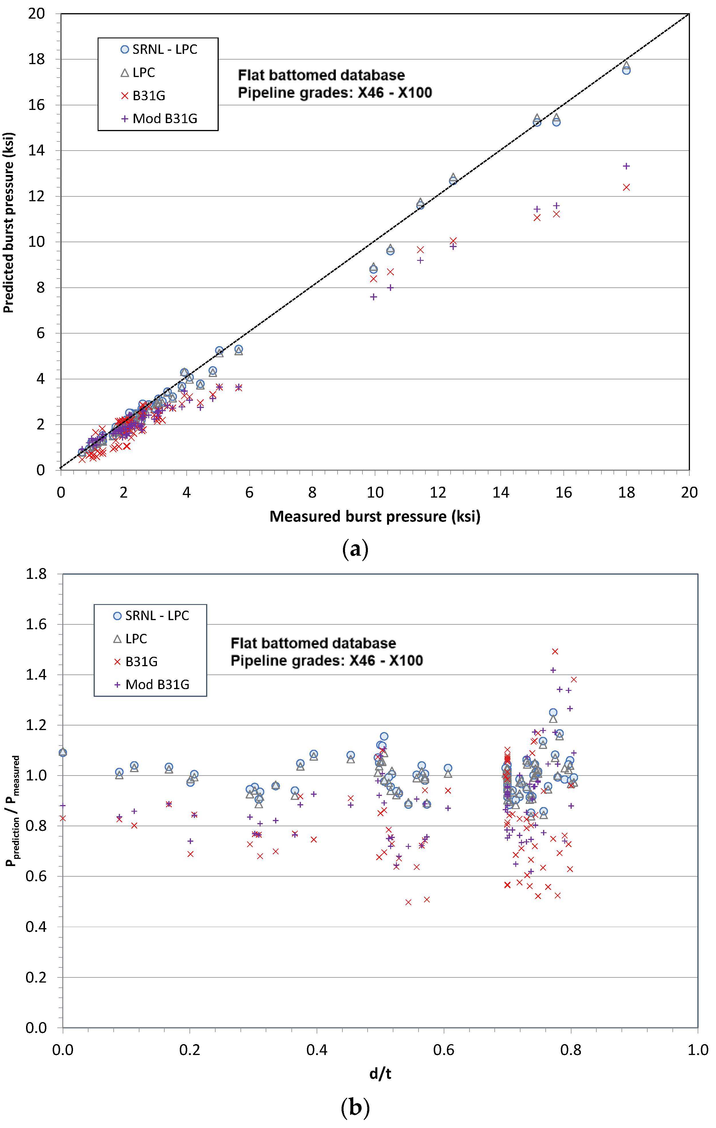
Figure 12a directly compares the burst pressure prediction from the LPC and SRNL-LPC models with the full-scale burst test data, while Figure 12b compares the burst pressure prediction to the experimental measurement ratio for different defect depth d/t ratios. Additionally included in these two figures are the burst pressure predictions of ASME B31G and Mod B31G. From these two figures, the following observations can be obtained:
- (1)
- ASME B31G generally predicts the most conservative burst pressures for almost all thin- and thick-walled pipes, except for very deep defects with the d/t ratio close to 0.8, where B31G overestimates burst pressures and leads to non-conservative predictions;
- (2)
- Mod B31G determines improved burst pressure predictions for most tests and reduces the conservatism in B31G. However, it can also predict non-conservative results for some tests;
- (3)
- LPC model significantly improves the predictions by both ASME B31G and Mod B31G and determines more accurate burst pressure for both thin- and thick-walled pipes. However, it can overestimate burst pressures for deep defects near d/t = 0.8;
- (4)
- SRNL-LPC model further improves LPC predictions and determines improved results for thin- and thick-walled pipes;
- (5)
- All models are inaccurate for deep defects near d/t = 0.8.
4.3. Machine Learning Models of Burst Pressure
Recall that Section 2.5 applied the machine learning technology with ANNs to model the burst pressure for defect-free pipes. Similarly, ANNs are employed to model the remaining strength of corroded thin- and thick-walled pipelines. All ANN approaches used for defect-free pipes are applicable to corroded pipes, and the defect width effect can be easily considered in ANN modeling. The only difference is that more input variables and hidden neurons are needed for modeling corroded pipes.
Figure 13 illustrates a typical ANN model for determining the burst pressure of corroded thin- and thick-walled pipelines. For defect-free pipes, the feature correlation analysis by Zhu et al. [33] showed that, for a burst strength analysis, there are two independent material parameters, UTS and n (or YS), and a pipe geometry parameter, D/t. For corroded pipes, a similar feature correlation analysis determines three additional defect geometry parameters: d/t, L/√(Dt), and W/D. As a result, there are six input variables, UTS, n, D/t, d/t, L/√(Dt), and W/D, for an ANN model to predict the output variable of burst pressure. For assumed hidden neurons and hidden layers, the best ANN model can be determined for a given training dataset, a validation dataset, and a test dataset. Our results on the ANN models of remaining burst strength for corroded thick-walled pipes have not been published yet and are not allowed to be discussed further. Due to this reason, a similar ANN model that was recently developed by Cai et al. [30] is discussed here for predicting the remaining strength of corroded pipelines.
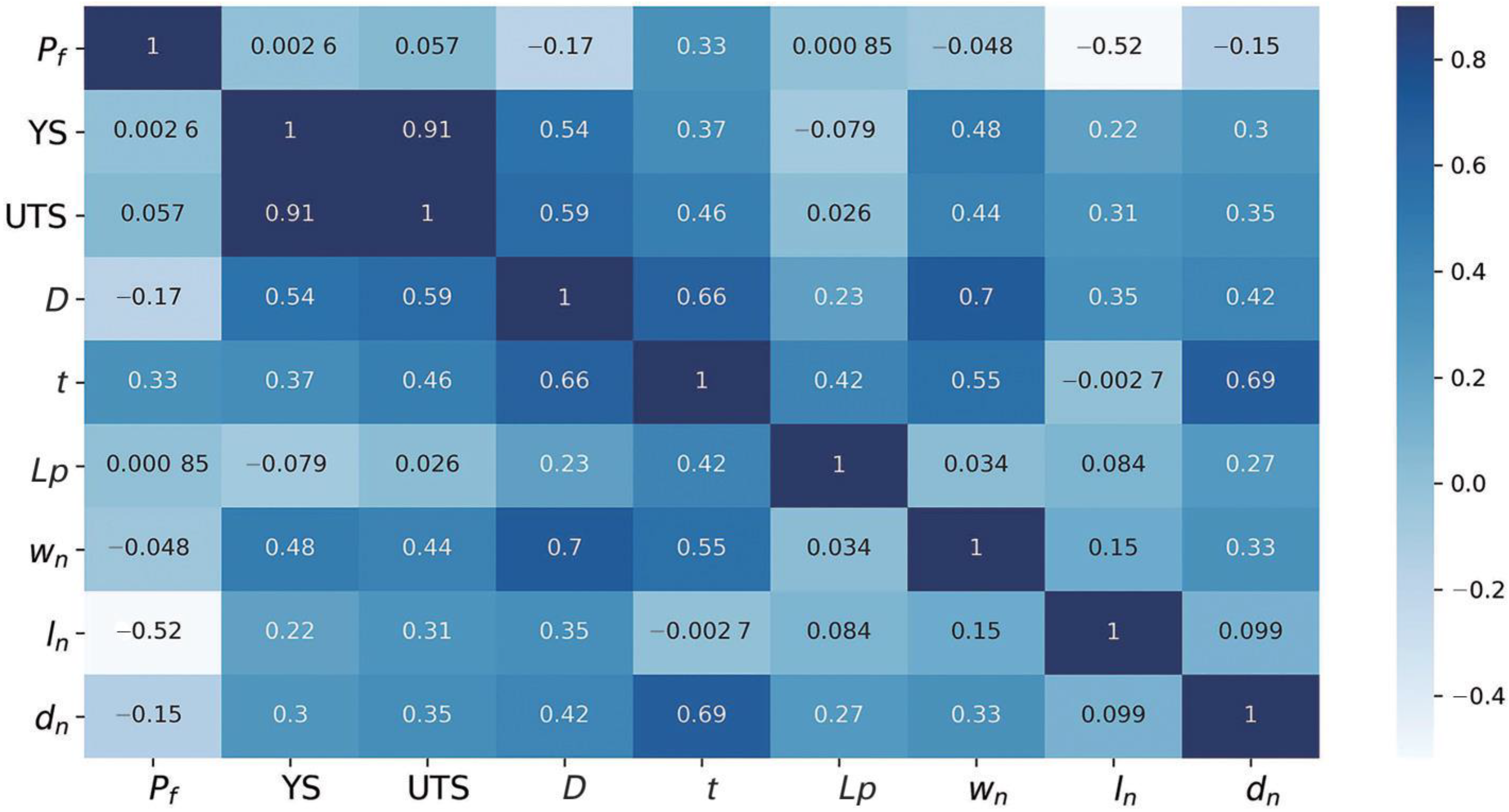
In machine learning, data exploration is essential for the proper training of a machine learning model. Cai et al. [30] considered nine variables for their experimental database, which contains 115 full-scale burst tests for a wide range of pipeline grades (Grade B, X42, X46, X52, X56, X60, X65, and X80). Two of them are the material properties (YS and UTS), three are pipe geometry sizes (D, t, pipeline length Lp), three are defect geometry sizes (length ln, depth dn, and width wn), and the last one is burst pressure Pf. Figure 14 shows the heatmap of the correlation coefficients of the pipe test variables from the experimental database. The legend of color denotes the level correlation. A value close to 1 implies a strong positive correlation between two features, while a value close to -1 implies a strong negative correction. The value of 0 indicates no correlation. The highly corrected features should be selected for machine learning. It was found that the variables of the pipe diameter (D), defect length (ln), and defect depth (dn) had a large negative correlation to the burst pressure, while the wall thickness (t) had a large positive correlation to the burst pressure. The pipe specimen length (Lp) and the corrosion width (wn) had a very small correlation value to the burst pressure, and, thus, these two features were intentionally removed from model training. As a result, six variables (YS, UTS, D, t, ln, dn) were selected as the input variables, and burst pressure was the output variable for ANN model training.
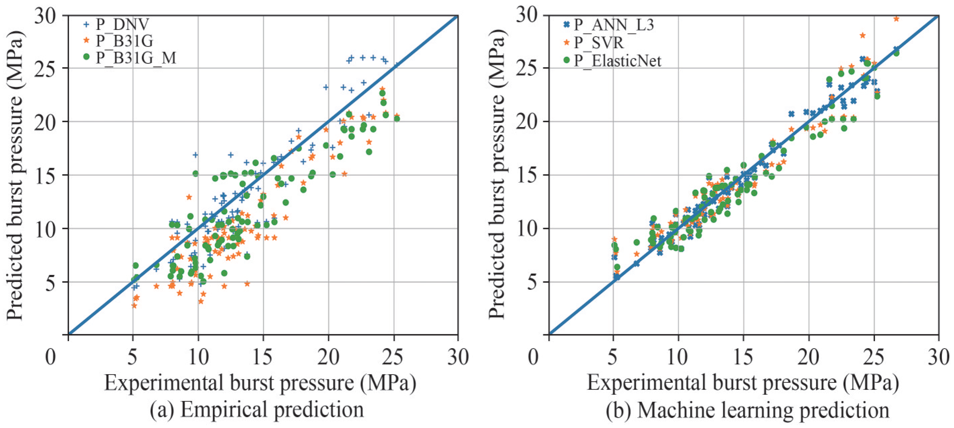
Figure 15 a and b compares the burst pressure predictions with experimental test data using three empirical prediction models and three machine learning methods, respectively. Figure 15a shows that the B31G predictions are conservative, the Mod B31G model has improved predictions, and the DNV model obtains overall better predictions on average. However, the DNV model has many overpredictions because it utilizes the reference stress of 1.05 UTS. In contrast to these empirical models, Figure 15b shows that the ANN-L3 model with three layers predicts the most accurate burst pressures for all steels in consideration. The other two machine learning models, namely, the linear regression with ElasticNet approach and the support vector regression (SVR), also predict acceptable results.
5. Major Technical Challenges and Gaps
5.1. Industry Need for Accurate Burst Prediciton Models
Usually, a conservative prediction model is accepted to determine a conservative failure pressure for pipeline design. However, Leis [69] pointed out that, if failure pressure is biased toward conservatism, as it has been historically, then, in order to balance this equation, that bias carries over inversely to the defect sizes. In other word, a conservative model determines a conservative failure pressure but a non-conservative defect size, as illustrated in Figure 8 of reference [69]. The regulations mandate scheduled rehabilitation based on defect severity, which can only be achieved through the use of accurate predictive severity criteria that, by definition, are unbiased. In this context, the SRNL-PCORRC and SRNL-LPC models can be used to assess either failure pressure or critical defect sizes at a given operating pressure. However, some uncertainty enters into such criteria due, for example, to model errors introduced by defect width or real defect shape. Recall that most of the corrosion models discussed previously are only applicable to rectangular defects and do not consider the defect width effect. This gap may lead to an increase in pipeline maintenance costs. It follows that the pipeline industry needs both accurate and precise prediction models for pipeline integrity assessment and management.
5.2. Full-Scale Burst Tests
Full-scale burst tests play a key role in the measurement of reliable burst pressure data. Usually, a full-scale hydrostatic test is conducted by filling water and pressuring it until failure of the pipe. However, such hydrostatic tests are expensive, particularly for large-diameter pipes, due to material and vessel manufacture costs. To reduce material costs, a short vessel may be utilized with a length of less than two times the diameter of the vessel. As a result, the short vessel may determine an inaccurate burst result that does not represent that of a long pipeline buried underground because the burst pressure measurement is likely elevated due to the capped-end effect. Such an effect is particularly true for a short vessel with a long defect. Therefore, a short vessel is not recommended for full-scale testing. In general, a pressure vessel should have at least five times the outside diameter to avoid the capped-end effect. A three-segment layout of a long pressure vessel has been designed as an option to solve the full-scale test challenge [21].
5.3. Numerical Simulation and Material Failure Criteria
The FEA calculation of pipeline failure is based on the continuum theory. However, this theory has no material failure criteria, and, thus, a prescribed material failure criterion is required in an FEA calculation to define material failure local to a defect. Different failure criteria [25,26,35,44,54,59,60,62,70,71,72] have been used in the FEA calculations of burst pressure for a pipeline with or without defects, which resulted in different predictions of burst pressure for the same pipe. The most often used material failure criteria include the RIKS instability model for determining global failure and some local failure criteria, such as the von Mises criteria, where the von Mises effective stress equals between 0.8 and 1.0 true UTS or 1.0 engineering UTS of the pipe steel. As such, developing an appropriate material failure criterion for the FEA calculations remains a great challenge or gap.
5.4. Assessment of Real Corrosion Defects
Assessing real metal-loss defects for buried pipelines faces numerous technical challenges for us. The first one is how to detect real defects in pipelines efficiently and how to characterize the sizes of irregular defects accurately. This needs advanced in-line inspection (ILI) technologies and inspection tools, such as magnetic flux leakage (MFL), ultrasonic technology (UT), and geometric tools, among others. Once a real corrosion defect is detected and characterized adequately, its accurate assessment is another big challenge. All real corrosion defects are not a single isolated, uniform defect but a cluster of corrosion pits with a river-bottom profile and may not be axially oriented. In addition, separate corrosion clusters may have interactions, as discussed in references [73,74,75,76]. Assessing corrosion–defect interaction is also a great challenge. For aged pipelines, material properties may not be well documented for all pipe segments. Estimating the material properties of unknown aged pipeline steels [77,78] can be an additional challenge for assessing corrosion defects for buried pipelines.
6. Conclusions
This paper presented a technical review of burst prediction models first for defect-free pipes and then for corroded pipes. The focus was on recent advances in corrosion assessment models for predicting the remaining burst strength of thin- and thick-walled pipelines. For a better understanding of corrosion assessment development, corrosion models were categorized into four generations and then evaluated using various full-scale burst test data. On this basis, the best burst prediction models were identified. Finally, major technical challenges and gaps were discussed for further investigation to improve pipeline integrity assessment and management.
For defect-free pipelines, a brief review was made of both the strength- and flow-theory-based solutions for predicting the burst pressure of thin-walled pipes, including the Tresca, von Mises, and Zhu–Leis solutions. The recent advances in burst model development include a new strength theory, a new theoretical flow solution, an advanced numerical model, and a machine learning model for predicting the burst pressure of thick-walled pipelines. Experimental data validated that the Zhu–Leis flow solution is accurate for defect-free thin and thick-walled pipelines.
For corroded pipelines, available corrosion assessment models were categorized into four generations in terms of the reference stress historically used in each model. The first three generation models were defined as when the flow stress, the UTS, or a combined function of the UTS and strain-hardening rate is used. The fourth-generation models were those recently developed at SRNL that embedded the Zhu–Leis burst strength for defect-free pipes and considered the wall-thickness effect. The full-scale burst data validated that Mod PCORRC and Mod LPC models are accurate for corroded thin-walled pipelines and that the SRNL-PCORRC and SRNL-LPC models are accurate for both thin- and thick-walled pipelines with corrosion or metal-loss defects.
Finally, major technical challenges and gaps were discussed, including the industry need for accurate burst prediction models, defect width effect, full-scale experimental tests of burst strength, FEA numerical simulation, material failure criteria, and irregular real corrosion defect assessment for buried, aged pipelines. It is anticipated that the fourth-generation models will serve as more efficient tools for real corrosion assessment and management of buried transmission pipelines.
Funding
This work was funded by the Laboratory Directed Research and Development (LDRD) program within the Savannah River National Laboratory (SRNL). This document was prepared in conjunction with work accomplished under contract no. 89303321CEM000080 with the U.S. Department of Energy (DOE) Office of Environmental Management (EM).
Informed Consent Statement
Not applicable.
Data Availability Statement
No new data were created in this work.
Acknowledgments
This author thanks the anonymous reviewers for their helpful comments.
Conflicts of Interest
The author declares no conflict of interest.
References
- Ahmed, S.K.; Kabir, G. An integrated approach for failure analysis of natural gas transmission pipeline. CivilEng 2021, 2, 87–119. [Google Scholar] [CrossRef]
- Dai, L.; Wang, D.; Wang, T. Analysis and comparison of long-distance pipeline failures. J. Pet. Eng. 2017, 2017, 3174636. [Google Scholar] [CrossRef] [Green Version]
- Nyman, D.J.; Lee, E.M.; Audibert, J.M.E. Mitigating geohazards for international pipeline projects: Challenges and lessons learned. In Proceedings of the 7th International Pipeline Conferences (IPC2008), Calgary, AB, Canada, 29 September–3 October 2008. [Google Scholar]
- Porter, M.; Ferris, G.; Leir, M.; Leach, M.; Haderspock, M. Updated estimates of frequencies of pipeline failures caused by geohazards. In Proceedings of the 11th International Pipeline Conferences (IPC2016), Calgary, AB, Canada, 26–30 September 2016. [Google Scholar]
- Peng, L.-C. Stress analysis methods for underground pipelines. Pipe Line Ind. 1978, 47, 67–71. [Google Scholar]
- American Lifeline AllianceAmerican Lifeline Alliance. Guidelines for the Design of Buried Steel Pipe; American Society of Civil Engineers: Reston, VA, USA, 2001. [Google Scholar]
- Christopher, T.; Sarma, B.S.; Potti, P.K. A comparative study on failure pressure estimation of unflawed cylindrical vessels. Int. J. Press. Vessel. Pip. 2002, 79, 53–66. [Google Scholar] [CrossRef]
- Law, M.; Bowie, G. Prediction of failure strain and burst pressure in high yield-to-tensile strength ratio line pipes. Int. J. Press. Vessel. Pip. 2007, 84, 487–492. [Google Scholar] [CrossRef]
- Zhu, X.K.; Leis, B.N. Evaluation of burst pressure prediction models for line pipes. Int. J. Press. Vessel. Pip. 2012, 89, 85–97. [Google Scholar] [CrossRef]
- Zhu, X.K.; Leis, B.N. Average shear stress yield criterion and its application to plastic collapse analysis of pipelines. Int. J. Press. Vessel. Pip. 2006, 83, 663–671. [Google Scholar] [CrossRef]
- Zhu, X.K.; Leis, B.N. Accurate prediction of burst pressure for line pipes. J. Pipeline Integr. 2004, 4, 195–206. [Google Scholar]
- Zhu, X.K. Strength criteria versus plastic flow criteria used in pressure vessel design and analysis. J. Press. Vessel. Technol. 2016, 138, 041402. [Google Scholar] [CrossRef]
- Kiefner, J.F.; Atterbury, T.J. Investigation of the Behavior of Corroded Line Pipe; Project 216 Interim Report to Texas Eastern Transmission Corporation; Battelle Memorial Institute: Columbus, OH, USA, 1971. [Google Scholar]
- Maxey, W.A.; Kiefner, J.F.; Eiber, R.J.; Duffy, A.R. Ductile fracture initiation, propagation and arrest in cylindrical vessels. In Fracture Toughness, ASTM STP 514, Part II; ASTM International: West Conshohocken, PA, USA, 1972; pp. 347–362. [Google Scholar]
- Kiefner, J.F.; Maxey, W.A.; Eiber, R.J.; Duffy, A.R. Failure stress levels of flaws in pressurized cylinders. In Progress in Flaw Growth and Fracture Toughness Testing, ASTM STP 536; American Society for Testing and Materials: West Conshohocken, PA, USA, 1973; pp. 461–481. [Google Scholar]
- ASME B31G-2009; Manual for Determining the Remaining Strength of Corroded Pipelines. American Society of Mechanical Engineers: New York, NY, USA, 2009.
- Cosham, A.; Hopkins, P.; Macdonald, K.A. Best practice for the assessment of defects in pipelines. Eng. Fail. Anal. 2007, 14, 1245–1265. [Google Scholar] [CrossRef]
- BS 7910-2013 + A1:2015; Methods for Accessing the Acceptability of Flaws in Metallic Structures. British Standards Institution: London, UK, 2015.
- API 579-1/ASME FFS-1; Fitness for Service, Third Edition. ASME: New York, NY, USA, 2016.
- Zhu, X.K. Assessment methods and technical challenges of remaining strength for corrosion defects in pipelines. In Proceedings of the ASME Pressure Vessels and Piping Conference (PVP2018), Prague, Czech Republic, 15–20 July 2018. [Google Scholar]
- Zhu, X.K. A Comparative Study of Burst Failure Models for Assessing Remaining Strength of Corroded Pipelines. J. Pipeline Sci. Eng. 2021, 1, 36–50. [Google Scholar] [CrossRef]
- Zhou, W.; Huang, G.X. Model error assessments of burst capacity models for corroded pipelines. Int. J. Press. Vessel. Pip. 2012, 99–100, 1–8. [Google Scholar] [CrossRef]
- Zhu, X.K. A new material failure criterion for numerical simulation of burst pressure of corrosion defects in pipelines. In Proceedings of the ASME Pressure Vessels and Piping Conference (PVP2025), Boston, MA, USA, 19–23 July 2015. [Google Scholar]
- Leis, B.N.; Zhu, X.K.; Orth, F.; Aguiar, D.; Perry, L. Minimize model uncertainty in current corrosion assessment criteria. In Proceedings of the PRCI-APGA-EPRG 21th Joint Technical Meeting on Pipeline Research, Colorado Springs, CO, USA, 1–5 May 2017. [Google Scholar]
- Heggab, A.; Nemr, A.E.; Aghoury, I.M. Numerical sensitivity analysis of corroded pipes and burst pressure prediction using finite element modeling. Int. J. Press. Vessel. Pip. 2023, 202, 104906. [Google Scholar] [CrossRef]
- Oh, D.H.; Race, J.; Oterkus, S.; Chang, E. A new methodology for the prediction of burst pressure for API 5L X grade flawless pipelines. Ocean Eng. 2020, 212, 107602. [Google Scholar] [CrossRef]
- Bhardwaj, U.; Teixeira, A.P.; Soares, C.G. Burst strength assessment of X100 to X120 ultra-high strength corroded pipes. Ocean Eng. 2021, 241, 110004. [Google Scholar] [CrossRef]
- Amaya-Gomez, R.; Sánchez-Silva, M.; Bastidas-Arteaga, E.; Schoefs, F.; Muñoz, F. Reliability assessments of corroded pipelines based on internal pressure—A review. Eng. Fail. Anal. 2019, 98, 190–214. [Google Scholar] [CrossRef]
- Bhardwaj, U.; Teixeira, A.P.; Soares, C.G. Uncertainty quantification of burst pressure models of corroded pipelines. Int. J. Press. Vessel. Pip. 2020, 188, 104208. [Google Scholar] [CrossRef]
- Cai, J.; Jiang, X.; Yang, Y.; Lodewijks, G.; Wang, M. Data-driven methods to predict the burst strength of corroded pipelines subjected to internal pressure. J. Mar. Sci. Appl. 2022, 21, 115–132. [Google Scholar] [CrossRef]
- Li, H.; Huang, K.; Zeng, Q.; Sun, C. Residual strength assessment and residual life prediction of corroded pipelines: A decade review. Energies 2022, 15, 726. [Google Scholar] [CrossRef]
- Zhu, X.K.; Wiersma, B.; Sindelar, R.; Johnson, W.R. New strength theory and its application to determine burst pressure of thick-wall pressure vessels. In Proceedings of the ASME 2022 Pressure Vessels and Piping Conference, Las Vegas, NV, USA, 17–22 July 2022. PVP2022-84902. [Google Scholar]
- Zhu, X.K.; Johnson, W.R.; Sindelar, R.; Wiersma, B. Artificial neural network models of burst strength for thin-wall pipelines. J. Pipeline Sci. Eng. 2022, 2, 100090. [Google Scholar] [CrossRef]
- Zhu, X.K.; Johnson, W.R.; Sindelar, R.; Wiersma, B. Machine learning models of burst strength for defect-free pipelines. In Proceedings of the ASME 2022 Pressure Vessels and Piping Conference, Las Vegas, NV, USA, 17–22 July 2022. PVP2022-84908. [Google Scholar]
- Johnson, W.R.; Zhu, X.K.; Sindelar, R.; Wiersma, B. Determining burst strength of thin and thick-walled pressure vessels through parametric finite element analysis. In Proceedings of the ASME 2023 Pressure Vessels and Piping Conference, Atlanta, GA, USA, 16–21 July 2023. PVP2023-106637. [Google Scholar]
- Zhu, X.K.; Wiersma, B. Progress of assessment model development for determining remaining strength of corroded pipelines. In Proceedings of the ASME 14th International Pipeline Conference, Calgary, AB, Canada, 26–30 September 2022. IPC2022-86922. [Google Scholar]
- Zhu, X.K.; Wiersma, B.; Johnson, W.R.; Sindelar, R. Corrosion assessment models for predicting remaining strength of corroded thick-walled pipelines. In Proceedings of the ASME 2023 Pressure Vessels and Piping Conference, Atlanta, GA, USA, 16–21 July 2023. PVP2023-106911. [Google Scholar]
- Zhu, X.K.; Leis, B.N. Influence of yield-to-tensile strength ratio on failure assessment of corroded pipelines. J. Press. Vessel. Technol. 2005, 127, 436–442. [Google Scholar] [CrossRef]
- Zimmermann, S.; Marewski, U.; Hohler, S. Burst pressure of flawless pipes. 3R Int. Spec. Ed. 2007, 46, 28–33. [Google Scholar]
- Zhou, W.; Huang, T. Model error assessment of burst capacity models for defect-free pipes. In Proceedings of the International Pipeline Conference (IPC2012), Calgary, AB, Canada, 25–28 September 2012. [Google Scholar]
- Bony, M.; Alamilla, J.L.; Vai, R.; Flores, E. Failure pressure in corroded pipelines based on equivalent solutions for undamaged pipe. J. Press. Vessel. Technol. 2010, 132, 051001. [Google Scholar] [CrossRef]
- Seghier, M.E.A.B.; Keshtegar, B.; Elahmoune, B. Reliability analysis of low, mid and high-grade strength corroded pipes based on plastic flow theory using adaptive nonlinear conjugate map. Eng. Fail. Anal. 2018, 90, 245–261. [Google Scholar] [CrossRef]
- Lyons, C.J.; Race, J.M.; Chang, E.; Cosham, A.; Wetenhall, B.; Barnett, J. Validation of the NG-18 Equations for thick-walled pipelines. Eng. Fail. Anal. 2020, 112, 104494. [Google Scholar] [CrossRef]
- Zhu, X.K.; Leis, B.N. Theoretical and numerical predictions of burst pressure of pipelines. J. Press. Vessel. Technol. 2007, 129, 644–652. [Google Scholar] [CrossRef]
- API Specification 5L. Lin Pipe, 46th ed.; American Petroleum Institute: Washington, DC, USA, 2018. [Google Scholar]
- Folias, E.S. An axial crack in a pressured cylindrical shell. Int. J. Fract. Mech. 1965, 1, 104–113. [Google Scholar] [CrossRef] [Green Version]
- Coulson, K.W.; Worthingham, R.G. Standard damage assessment approach is overly conservative. Oil Gas J. 1990, 88, 15. [Google Scholar]
- Kiefner, J.F.; Vieth, P.H. A Modified Criterion for Evaluating the Remaining Strength of Corroded Pipe; Final Report on Project PR 3-805 to the Pipeline Research Committee of the American Gas Association; Battelle Memorial Institute: Columbus, OH, USA, 1989. [Google Scholar]
- Kiefner, J.F.; Vieth, P.H.; Roytman, I. Continuing Validation of RSTRENG; Pipeline Research Supervisory Committee, A.G.A Catalogue No. L51689; Kiefner and Associates, Inc.: Worthington, OH, USA, 1996. [Google Scholar]
- Ma, B.; Shuai, J.; Wang, J.; Han, K. Analysis on the latest assessment criteria of ASME B31G-2009 for the remaining strength of corroded pipelines. J. Fail. Anal. Prev. 2011, 11, 666–667. [Google Scholar] [CrossRef]
- Yan, J.; Lu, D.; Zhou, I.; Zhang, S. A more efficient effective area method algorithm for corrosion assessment (Faster RSTRENG). In Proceeding of the 14 International Pipeline Conference (IPC2022), Calgary, AB, Canada, 26–30 September 2022. [Google Scholar]
- Ritchie, D.; Last, S. Shell 92—Burst criteria of corroded pipelines—Defect acceptance criteria. In Proceedings of the EPRG-PRCI 10th Biannual Joint Technical Meeting on Pipeline Research, Cambridge, UK, 18–21 April 1995. [Google Scholar]
- CSA Z662-19; Oil and Gas Pipeline Systems. Canadian Standards Association: Mississauga, ON, Canada, 2019.
- Fu, B.; Kirkwood, M.G. Determination of failure pressure of corroded linepipes using nonlinear finite element method. In Proceedings of the 2nd International Pipeline Technology Conference, Ostend, Belgium, 11–14 September 1995; Volume II, pp. 1–9. [Google Scholar]
- Fu, B.; Batte, A.D. New methods for assessing the remaining strength of corroded pipelines. In Proceedings of the EPRG/PRCI 12th Biennial Joint Technical Meeting on Pipeline Research, Groningen, The Netherlands, 17–21 May 1999. Paper 28. [Google Scholar]
- Det Norske Veritas. Recommended Practice DNV-RP-F101—Corroded Pipelines; Det Norske Veritas: Hovik, Norway, 2015. [Google Scholar]
- Leis, B.N.; Stephens, D.R. An alternative approach to assess the integrity of corroded line pipes—Part I: Current status and Part II: Alternative criterion. In Proceedings of the Seventh International Offshore and Polar Engineering Conference, Honolulu, HI, USA, 25–30 May 1997. [Google Scholar]
- Stephens, D.R.; Leis, B.N. Development of an alternative criterion for residual strength of corrosion defects in moderate-to-high toughness pipe. In Proceedings of the International Pipeline Conference, Calgary, AB, Canada, 1–5 October 2000. [Google Scholar]
- Choi, J.B.; Goo, B.K.; Kim, J.C.; Kim, Y.; Kim, W. Development of limit load solutions for corroded gas pipelines. Int. J. Press. Vessel. Pip. 2003, 80, 121–128. [Google Scholar] [CrossRef]
- Yeom, K.J.; Lee, Y.-K.; Oh, K.H.; Kim, W.S. Integrity assessment of a corroded API X70 pipe with a single defect by burst pressure analysis. Eng. Fail. Anal. 2015, 57, 553–561. [Google Scholar] [CrossRef]
- Chauhan, V.; Brister, J. A Review of Methods for Assessing the Remaining Strength of Corroded Pipelines; US DOT Final Report 153A; National Academy of Sciences: Washington, DC, USA, 2009. [Google Scholar]
- Ma, B.; Shuai, J.; Liu, D.; Xu, K. Assessment on failure pressure of high strength pipeline with corrosion defects. Eng. Fail. Anal. 2013, 32, 209–219. [Google Scholar] [CrossRef]
- Zhu, X.K. Burst failure models and their predictions of buried pipelines. In Proceedings of the Conference on Asset Integrity Management—Pipeline Integrity Management under Geohazard Conditions, Houston, TX, USA, 25–28 March 2019. [Google Scholar]
- Kim, W.S.; Kim, Y.P.; Kho, Y.T.; Choi, J.B. Full scale burst test and finite element analysis on corroded gas pipeline. In Proceedings of the Fourth International Pipeline Conference, Calgary, AB, Canada, 30 September–3 October 2002. [Google Scholar]
- Leis, B.N. Continuing Development of Metal-Loss Severity Criteria—Including Width Effects. In Proceedings of the ASME International Pipeline Conference, Calgary, AB, Canada, 30 September–3 October 2020. [Google Scholar]
- Chin, K.T.; Arumugam, T.; Karuppanan, S.; Ovinis, M. Failure pressure prediction of pipeline with single corrosion defects using artificial neural network. Pipeline Sci. Technol. 2020, 4, 10–17. [Google Scholar] [CrossRef]
- Ossai, C.I. Corrosion defect modeling of aged pipelines with a feed-forward multi-layer neural network for leak and burst failure estimation. Eng. Fail. Anal. 2020, 110, 104397. [Google Scholar] [CrossRef]
- Lo, M.; Karuppanan, S.; Ovinis, M. ANN-and FEA-based assessment equation for a corroded pipeline with a single corrosion defect. J. Mar. Sci. Eng. 2022, 10, 476. [Google Scholar] [CrossRef]
- Lies, B.N. Evolution of metal-loss severity criteria: Gaps and forward. J. Pipeline Sci. Eng. 2021, 1, 51–62. [Google Scholar] [CrossRef]
- Besel, M.; Zimmermann, S.; Kalwa, C.; Liessem, A. Corrosion assessment method validation for high-grade line pipe. In Proceeding of the 8th Int Pipeline Conference, Calgary, AB, Canada, 27 September–1 October 2010. [Google Scholar]
- Chiodo, M.S.G.; Ruggieri, C. Failure assessments of corroded pipelines with axial defects using stress-based criteria: Numerical studies and verification analyses. Int. J. Press. Vessel. Pip. 2009, 86, 164–176. [Google Scholar] [CrossRef]
- Velazquesz, J.C.; Gonzalez-Arevalo, N.E.; Diaz-Cruz, M.; Cervantes-Tobón, A.; Herrera-Hernández, H.; Hernández-Sánchez, E. Failure pressure estimation for an aged and corroded oil and gas pipelines: A finite element study. J. Nat. Gas Sci. Eng. 2022, 101, 104532. [Google Scholar] [CrossRef]
- Sun, J.; Cheng, Y.F. Assessment by finite element modeling of the interaction of multiple corrosion defects and the effect on failure pressure of corroded pipelines. Eng. Struct. 2018, 165, 278–286. [Google Scholar] [CrossRef]
- Idris, N.N.; Mustaffa, Z.; Seghier, M.E.; Trung, N.T. Burst capacity and development of interaction rules for pipelines considering radial interacting corrosion defects. Eng. Fail. Anal. 2021, 121, 105124. [Google Scholar] [CrossRef]
- Wang, W.; Zhang, Y.; Shuai, J.; Shuai, Y.; Shi, L.; Lv, Z.Y. Mechanical Synergistic Interaction between Adjacent Corrosion Defects and Its Effect on Pipeline Failure. Pet. Sci. 2023, in press. [CrossRef]
- Sun, M.; Fang, H.; Miao, Y.; Zhao, H.; Li, X. Experimental Study on Strain and Failure Location of Interacting Defects in Pipeline. Eng. Fail. Anal. 2023, 107119, in press. [Google Scholar] [CrossRef]
- Smart, L.J.; Engle, B.J.; Bond, L.J.; Machenzie, J.; Morris, G. Material characterization of pipeline steels: Inspection techniques review and potential property relationships. In Proceedings of the International Pipeline Conference, Calgary, AL, Canada, 26–30 September 2016. [Google Scholar]
- Martin, L.P.; Switzner, N.T.; Oneal, O.; Curiel, S.; Anderson, J.; Veloo, P. Quantitative evaluation of microstructure to support verification of material properties in line-pipe steels. In Proceedings of the International Pipeline Conference, Calgary, AL, Canada, 26–30 September 2022. [Google Scholar]
Figure 1.
A gas pipeline being buried in construction.

Figure 2.
Comparison of three flow solutions and experimental data for various carbon steels.

Figure 3.
Comparison of three geometry terms used in the burst pressure solutions [32].
Figure 3.
Comparison of three geometry terms used in the burst pressure solutions [32].

Figure 4.
Comparison of predicted and measured burst pressures in the function of D/t [32].
Figure 4.
Comparison of predicted and measured burst pressures in the function of D/t [32].

Figure 5.
Numerical burst pressure normalized by the thick-walled Tresca strength solution as a function of the strain-hardening exponent n for all 60 FEA cases [35].
Figure 5.
Numerical burst pressure normalized by the thick-walled Tresca strength solution as a function of the strain-hardening exponent n for all 60 FEA cases [35].

Figure 6.
Architecture of ANN model 2 [33].
Figure 6.
Architecture of ANN model 2 [33].

Figure 7.
Comparison of predicted and measured burst strengths for all full-scale tests [33].
Figure 7.
Comparison of predicted and measured burst strengths for all full-scale tests [33].

Figure 8.
Comparison of the second-generation corrosion models for X65 [21].
Figure 8.
Comparison of the second-generation corrosion models for X65 [21].

Figure 9.
Comparison of LPC, PCORRC, and their modified models for X70.

Figure 10.
Comparison of third-generation corrosion model predictions with test data [21].
Figure 10.
Comparison of third-generation corrosion model predictions with test data [21].

Figure 11.
Comparison of the M-PCORRC predictions with the experimental data for machined defects in modern pipeline grades ranging from X52 to X100 [65].
Figure 11.
Comparison of the M-PCORRC predictions with the experimental data for machined defects in modern pipeline grades ranging from X52 to X100 [65].

Figure 12.
Comparison of LPC and SRNL-LPC model predictions with experimental burst data: (a) direct comparison and (b) the pressure ratio as a function of d/t [37].
Figure 12.
Comparison of LPC and SRNL-LPC model predictions with experimental burst data: (a) direct comparison and (b) the pressure ratio as a function of d/t [37].

Figure 13.
Illustration of a typical ANN model for corroded pipes.

Figure 14.
Correlation coefficients among pipe burst pressure and pipe test feature [30].
Figure 14.
Correlation coefficients among pipe burst pressure and pipe test feature [30].

Figure 15.
Comparison of burst pressure predictions with test data for corroded pipes [30].
Figure 15.
Comparison of burst pressure predictions with test data for corroded pipes [30].

Disclaimer/Publisher’s Note: The statements, opinions and data contained in all publications are solely those of the individual author(s) and contributor(s) and not of MDPI and/or the editor(s). MDPI and/or the editor(s) disclaim responsibility for any injury to people or property resulting from any ideas, methods, instructions or products referred to in the content. |
© 2023 by the author. Licensee MDPI, Basel, Switzerland. This article is an open access article distributed under the terms and conditions of the Creative Commons Attribution (CC BY) license (https://creativecommons.org/licenses/by/4.0/).
Share and Cite
MDPI and ACS Style
Zhu, X.-K. Recent Advances in Corrosion Assessment Models for Buried Transmission Pipelines. CivilEng 2023, 4, 391-415. https://doi.org/10.3390/civileng4020023
AMA Style
Zhu X-K. Recent Advances in Corrosion Assessment Models for Buried Transmission Pipelines. CivilEng. 2023; 4(2):391-415. https://doi.org/10.3390/civileng4020023
Chicago/Turabian StyleZhu, Xian-Kui. 2023. "Recent Advances in Corrosion Assessment Models for Buried Transmission Pipelines" CivilEng 4, no. 2: 391-415. https://doi.org/10.3390/civileng4020023