
Site-Specific Response Spectra: Guidelines for Engineering Practice

 ,
,
Abstract
:1. Introduction
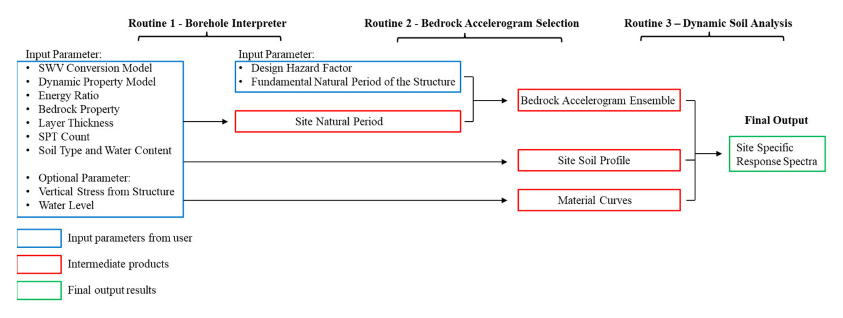
2. Overview of Analyses Required for Developing a Site-Specific Response Spectrum
3. Modelling Shear Wave Velocity and Dynamic Properties of Soil and Bedrock
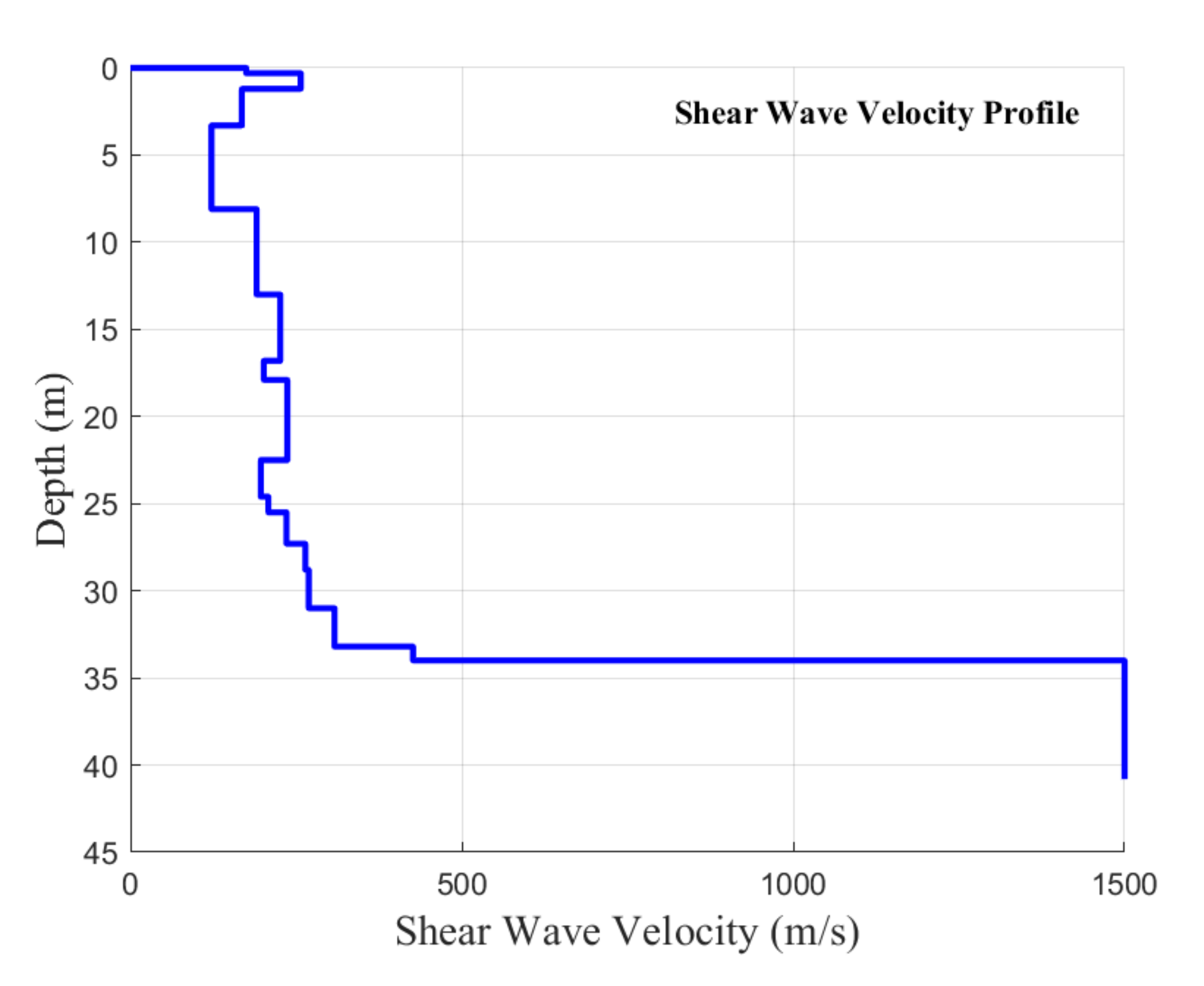
3.1. Shear Wave Velocity
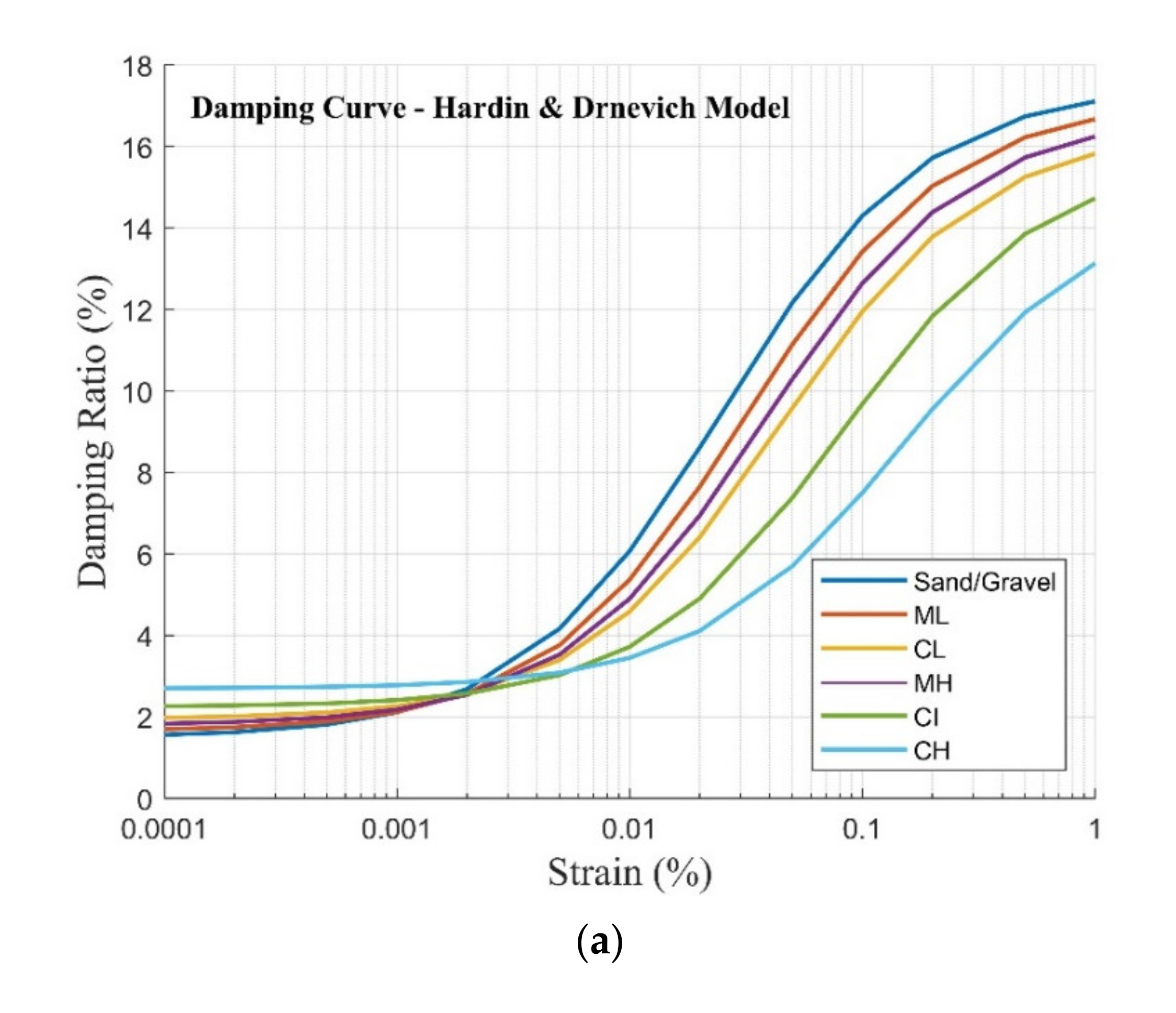
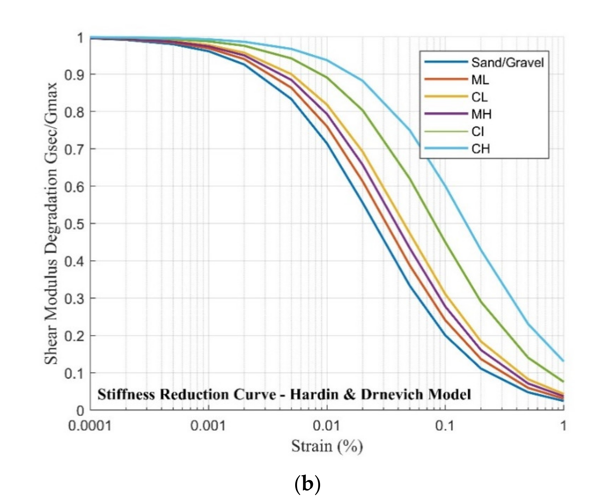
3.2. Soil Dynamic Property
3.3. Bedrock Property
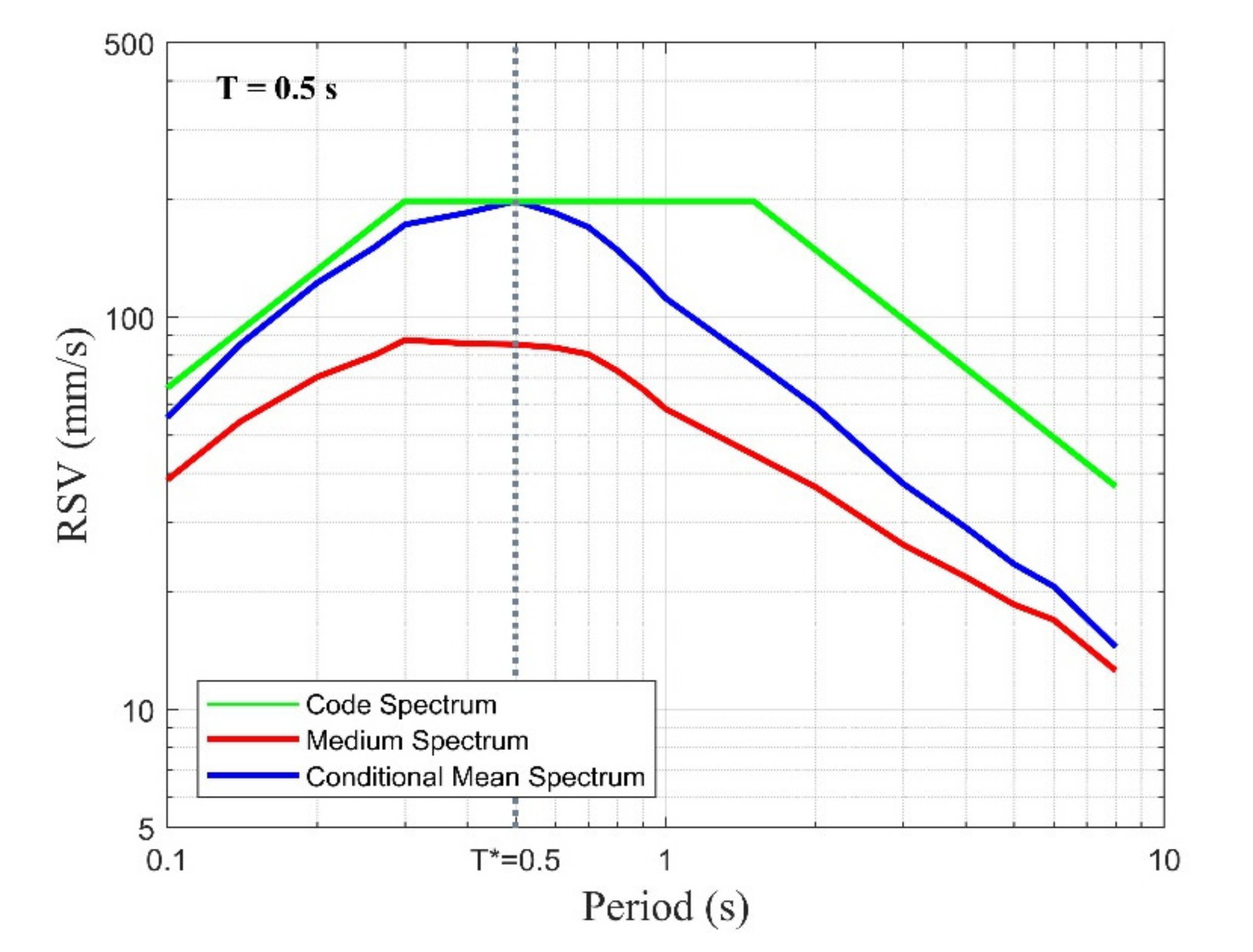
4. Accelerograms for Defining Input Motion at the Bedrock Level
- Style of faulting: reverse/oblique (typical of intraplate earthquakes);
- Magnitude: magnitude range (half-bin width) of centered at the magnitude of the controlling scenarios;
- Joyner–Boore distance Rjb (distance to the fault projection to the surface): distance range (half-bin width) of centered at the distance of the controlling scenarios (with the range extended to at );
- : to representing rock conditions.
5. Dynamic Analysis of the Soil Column Model
6. Case Study
7. Conclusions
Author Contributions
Funding
Acknowledgments
Conflicts of Interest
Appendix A. Density

| (a) | |||||||||||||||
| Soil Type | Water Content | ||||||||||||||
| M1 | M2 | M3 | W1 | W2 | |||||||||||
| ML | 1.49 | 1.59 | 1.6 | 1.59 | 1.6 | ||||||||||
| MH | 1.59 | 1.61 | 1.65 | 1.73 | 1.72 | ||||||||||
| CL | 1.41 | 1.44 | 1.49 | 1.61 | 1.54 | ||||||||||
| CI | 1.44 | 1.51 | 1.6 | 1.61 | 1.64 | ||||||||||
| CH | 1.6 | 1.72 | 1.54 | 1.64 | 1.72 | ||||||||||
| (b) | |||||||||||||||
| Soil Type | Water Content | ||||||||||||||
| Dry | Moist | Wet | |||||||||||||
| Relative Density | Relative Density | Relative Density | |||||||||||||
| VL | L | MD | D | VD | VL | L | MD | D | VD | VL | L | MD | D | VD | |
| GP | 1.79 | 1.83 | 1.91 | 1.99 | 2.04 | 1.95 | 1.99 | 2.05 | 2.12 | 2.16 | 2.11 | 2.14 | 2.19 | 2.24 | 2.27 |
| GW | 1.80 | 1.86 | 1.97 | 2.1 | 2.18 | 1.96 | 2.01 | 2.10 | 2.2 | 2.27 | 2.12 | 2.16 | 2.23 | 2.31 | 2.36 |
| GM | 1.64 | 1.7 | 1.81 | 1.94 | 2.02 | 1.83 | 1.88 | 1.97 | 2.07 | 2.14 | 2.02 | 2.06 | 2.13 | 2.21 | 2.26 |
| GC | 1.64 | 1.7 | 1.81 | 1.94 | 2.02 | 1.83 | 1.88 | 1.97 | 2.07 | 2.14 | 2.02 | 2.06 | 2.13 | 2.21 | 2.26 |
| SP | 1.56 | 1.62 | 1.73 | 1.86 | 1.94 | 1.76 | 1.81 | 1.90 | 2.01 | 2.07 | 1.97 | 2.01 | 2.08 | 2.16 | 2.21 |
| SW | 1.57 | 1.64 | 1.79 | 1.96 | 2.07 | 1.77 | 1.83 | 1.95 | 2.09 | 2.18 | 1.98 | 2.02 | 2.11 | 2.22 | 2.29 |
| SM | 1.34 | 1.43 | 1.61 | 1.84 | 2.02 | 1.58 | 1.66 | 1.81 | 2.00 | 2.14 | 1.83 | 1.89 | 2.00 | 2.15 | 2.26 |
| SC | 1.41 | 1.49 | 1.65 | 1.84 | 1.98 | 1.64 | 1.71 | 1.84 | 1.99 | 2.1 | 1.88 | 1.93 | 2.02 | 2.14 | 2.23 |
Appendix B. Dynamic Properties
- (1)
- Vucetic and Dobry model
| (a) | ||||
| Stiffness Degradation Curve | ||||
| Shear Strain (%) | PI = 0 | PI = 15 | PI = 30 | PI = 50 |
| 0.00001 | 1 | 1 | 1 | 1 |
| 0.0001 | 1 | 1 | 1 | 1 |
| 0.0002 | 1 | 1 | 1 | 1 |
| 0.0005 | 0.99 | 1 | 1 | 1 |
| 0.001 | 0.984 | 0.992 | 1 | 1 |
| 0.002 | 0.916 | 0.965 | 0.992 | 1 |
| 0.005 | 0.818 | 0.898 | 0.953 | 0.982 |
| 0.01 | 0.711 | 0.818 | 0.898 | 0.953 |
| 0.02 | 0.578 | 0.719 | 0.816 | 0.898 |
| 0.05 | 0.381 | 0.549 | 0.664 | 0.781 |
| 0.1 | 0.256 | 0.408 | 0.537 | 0.676 |
| 0.2 | 0.16 | 0.287 | 0.416 | 0.535 |
| 0.5 | 0.067 | 0.158 | 0.266 | 0.377 |
| 1 | 0.027 | 0.096 | 0.162 | 0.246 |
| 2 | 0.008 | 0.055 | 0.09 | 0.135 |
| 5 | 0.004 | 0.028 | 0.045 | 0.068 |
| (b) | ||||
| Damping Curve (%) | ||||
| Shear Strain (%) | PI = 0 | PI = 15 | PI = 30 | PI = 50 |
| 0.00001 | 1.0 | 1.0 | 1.0 | 0.9 |
| 0.0001 | 1.2 | 1.1 | 1.0 | 1.0 |
| 0.0002 | 1.2 | 1.2 | 1.1 | 1.0 |
| 0.0005 | 0.5 | 1.3 | 1.2 | 1.1 |
| 0.001 | 1.8 | 1.6 | 1.4 | 1.3 |
| 0.002 | 2.5 | 2.1 | 1.7 | 1.6 |
| 0.005 | 3.8 | 3.2 | 2.7 | 2.3 |
| 0.01 | 5.4 | 4.6 | 3.7 | 2.9 |
| 0.02 | 7.8 | 6.3 | 5.0 | 3.7 |
| 0.05 | 12.0 | 9.1 | 6.9 | 4.9 |
| 0.1 | 15.2 | 11.6 | 8.6 | 6.1 |
| 0.2 | 18.4 | 14.2 | 10.8 | 7.8 |
| 0.5 | 21.8 | 17.7 | 14.1 | 10.9 |
| 1 | 23.9 | 20.0 | 16.9 | 13.4 |
| 2 | 25.4 | 22.1 | 19.9 | 16.3 |
| 5 | 26.7 | 24.3 | 22.6 | 19.2 |
- (2)
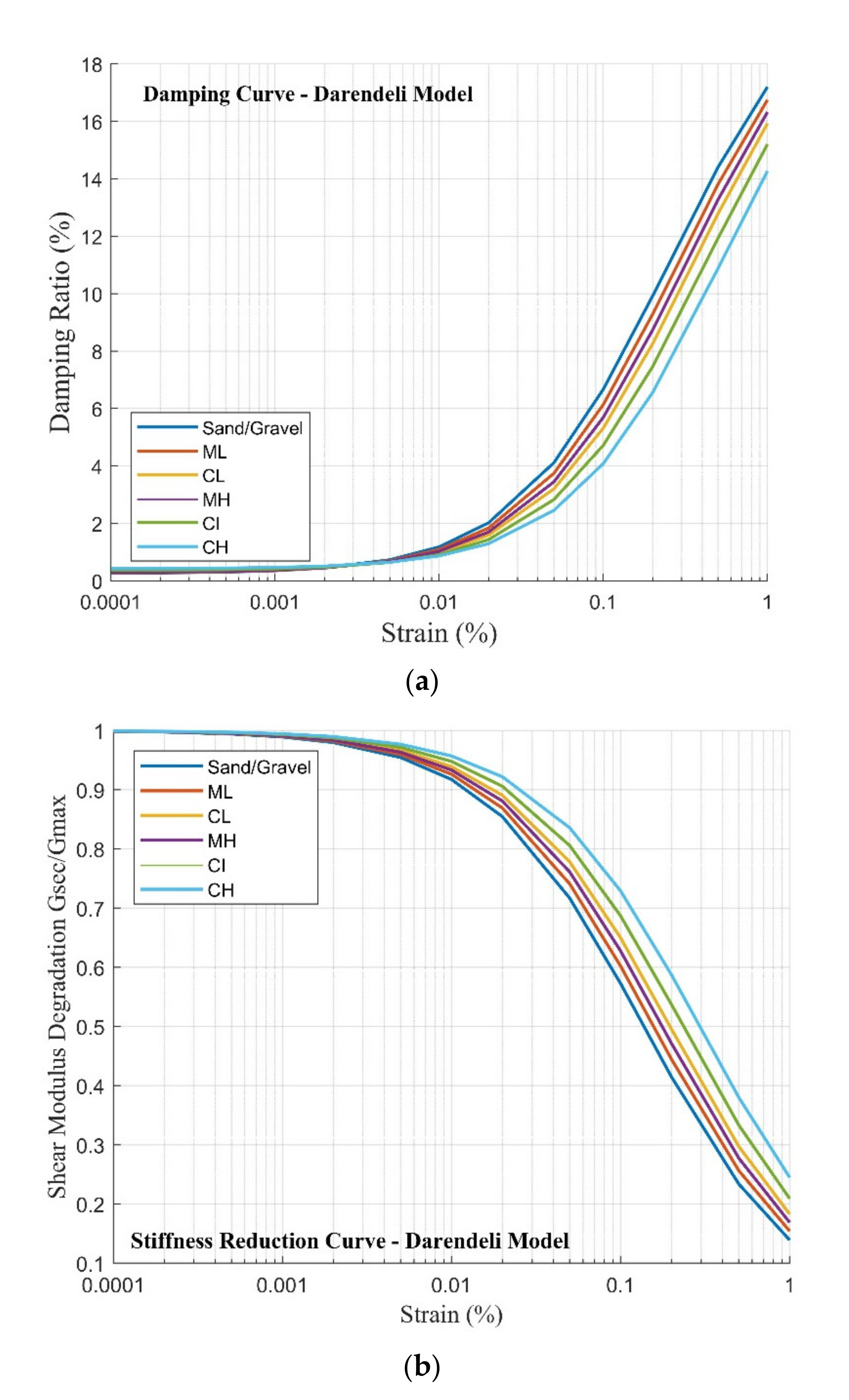
- The Darendeli model

- (3)
- Dynamic properties for bedrock
| Stiffness Degradation Curve | Damping Curve | ||
|---|---|---|---|
| Shear Strain (%) | Shear Strain (%) | Damping Ratio (%) | |
| 0.000001 | 1 | 0.000001 | 0.01 |
| 0.00001 | 1 | 0.00001 | 0.1 |
| 0.0001 | 1 | 0.0001 | 0.4 |
| 0.0003 | 1 | 0.001 | 0.8 |
| 0.001 | 0.9875 | 0.01 | 1.5 |
| 0.003 | 0.9525 | 0.1 | 3 |
| 0.01 | 0.9 | 1 | 4.6 |
| 0.03 | 0.81 | ||
| 0.1 | 0.725 | ||
| 1 | 0.55 | ||
| 10 | 0.2 | ||
| 100 | 0.1 | ||
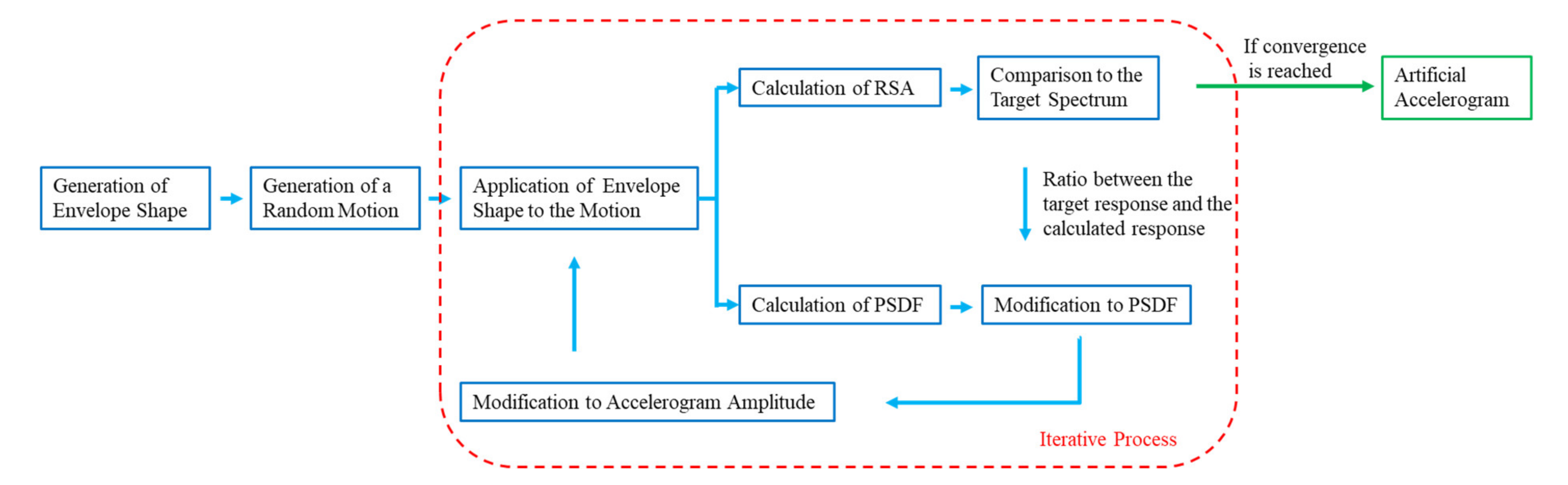
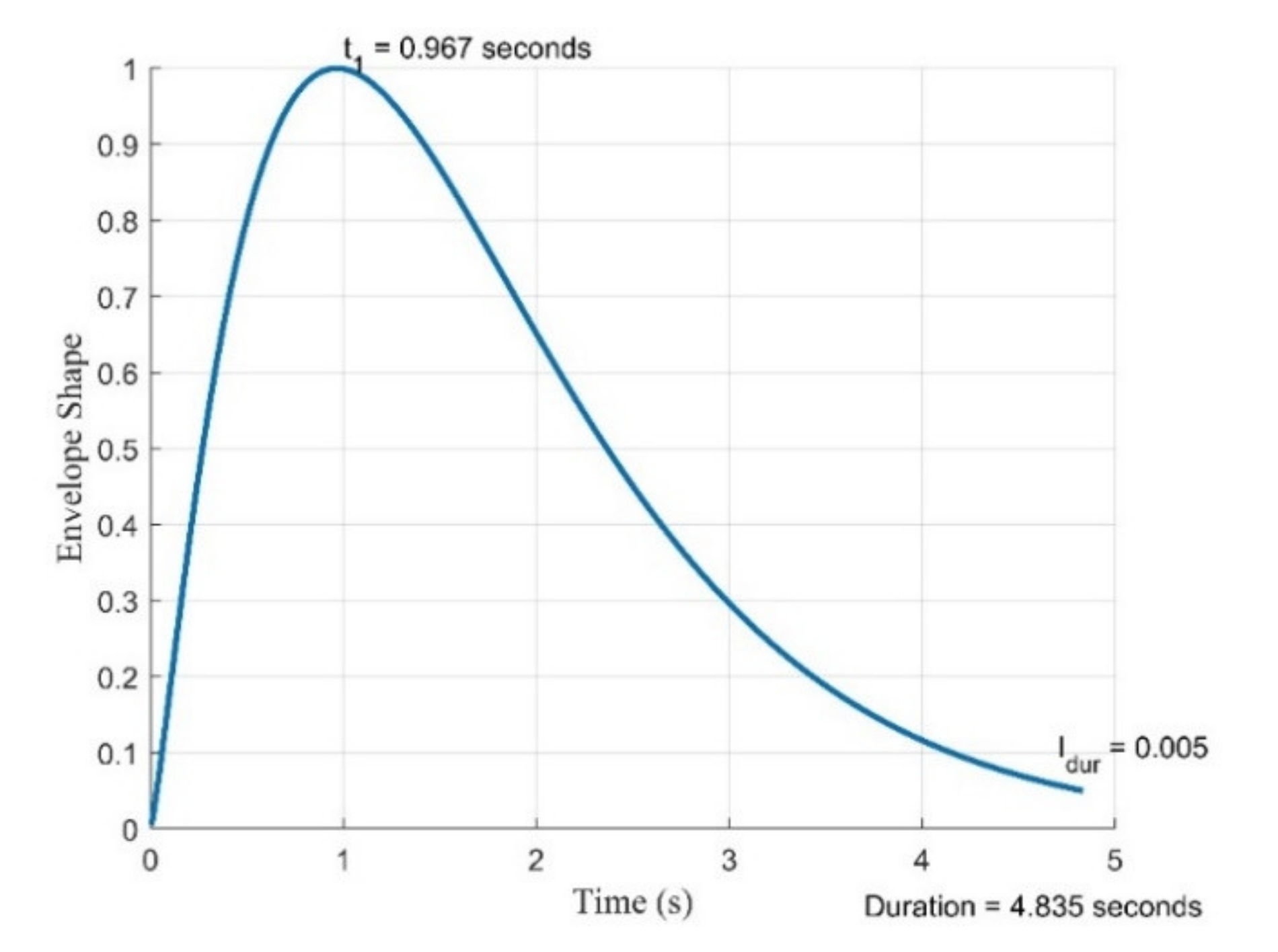
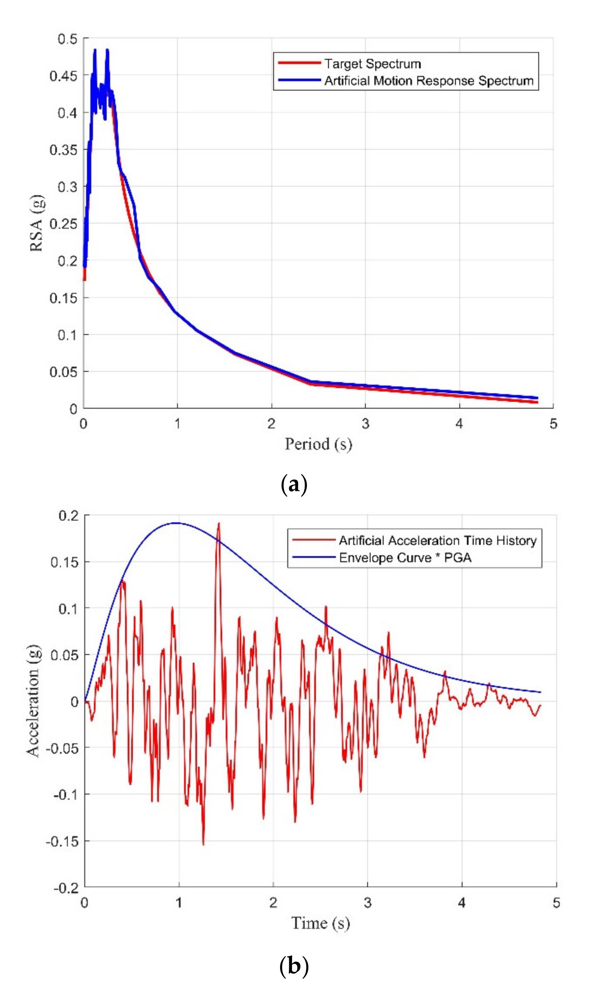
Appendix C. Artificial Ground Motion Accelerograms

- (1)
- (2)
- Peak time corresponds to the time at which the amplitude of the ground motion reaches the peak, meaning that the envelope function (representing the normalized amplitude) equals to unity at this point. The value of may be taken as by default.
- (3)
- may be taken as 0.05 by default.


References
- AS 1170. 4-2007 Structural Design Actions. In Part 4: Earthquake Actions in Australia; Standards Australia: Sydney, Australia, 2007. [Google Scholar]
- Dhakal, R.P.; Lin, S.-L.; Loye, A.K.; Evans, S.J. Seismic design spectra for different soil classes. Bull. N. Z. Soc. Earthq. Eng. 2013, 46, 79–87. [Google Scholar] [CrossRef]
- Calzolari, C.; Ungaro, F. Predicting shallow water table depth at regional scale from rainfall and soil data. J. Hydrol. 2012, 414, 374–387. [Google Scholar] [CrossRef]
- Forcellini, D. The Role of the Water Level in the Assessment of Seismic Vulnerability for the 23 November 1980 Irpinia–Basilicata Earthquake. Geosciences 2020, 10, 229. [Google Scholar] [CrossRef]
- Mina, D.; Forcellini, D. Soil–structure interaction assessment of the 23 November 1980 Irpinia-Basilicata earthquake. Geosciences 2020, 10, 152. [Google Scholar] [CrossRef] [Green Version]
- Simonson, G.; Boersma, L. Soil morphology and water table relations: II. Correlation between annual water table fluctuations and profile features. Soil Sci. Soc. Am. J. 1972, 36, 649–653. [Google Scholar] [CrossRef]
- Gatmiri, B.; Arson, C. Seismic site effects by an optimized 2D BE/FE method II. Quantification of site effects in two-dimensional sedimentary valleys. Soil Dyn. Earthq. Eng. 2008, 28, 646–661. [Google Scholar] [CrossRef]
- Luo, Y.; Fan, X.; Huang, R.; Wang, Y.; Yunus, A.P.; Havenith, H.-B. Topographic and near-surface stratigraphic amplification of the seismic response of a mountain slope revealed by field monitoring and numerical simulations. Eng. Geol. 2020, 271, 105607. [Google Scholar] [CrossRef]
- Maufroy, E.; Chaljub, E.; Hollender, F.; Kristek, J.; Moczo, P.; Klin, P.; Priolo, E.; Iwaki, A.; Iwata, T.; Etienne, V. Earthquake ground motion in the Mygdonian basin, Greece: The E2VP verification and validation of 3D numerical simulation up to 4 Hz. Bull. Seismol. Soc. Am. 2015, 105, 1398–1418. [Google Scholar] [CrossRef] [Green Version]
- Moczo, P.; Kristek, J.; Bard, P.-Y.; Stripajová, S.; Hollender, F.; Chovanová, Z.; Kristeková, M.; Sicilia, D. Key structural parameters affecting earthquake ground motion in 2D and 3D sedimentary structures. Bull. Earthq. Eng. 2018, 16, 2421–2450. [Google Scholar] [CrossRef] [Green Version]
- Tsang, H.; Wilson, J.; Lam, N.; Su, R. A design spectrum model for flexible soil sites in regions of low-to-moderate seismicity. Soil Dyn. Earthq. Eng. 2017, 92, 36–45. [Google Scholar] [CrossRef] [Green Version]
- Bindi, D.; Massa, M.; Luzi, L.; Ameri, G.; Pacor, F.; Puglia, R.; Augliera, P. Pan-European ground-motion prediction equations for the average horizontal component of PGA, PGV, and 5%-damped PSA at spectral periods up to 3.0 s using the RESORCE dataset. Bull. Earthq. Eng. 2014, 12, 391–430. [Google Scholar] [CrossRef] [Green Version]
- Falcone, G.; Acunzo, G.; Mendicelli, A.; Mori, F.; Naso, G.; Peronace, E.; Porchia, A.; Romagnoli, G.; Tarquini, E.; Moscatelli, M. Seismic amplification maps of Italy based on site-specific microzonation dataset and one-dimensional numerical approach. Eng. Geol. 2021, 289, 106170. [Google Scholar] [CrossRef]
- Yi, J.; Lam, N.; Tsang, H.-H.; Au, F.T. Selection of earthquake ground motion accelerograms for structural design in Hong Kong. Adv. Struct. Eng. 2020, 23, 2044–2056. [Google Scholar] [CrossRef]
- Baker, J.W.; Cornell, C. Spectral shape, epsilon and record selection. Earthq. Eng. Struct. Dyn. 2006, 35, 1077–1095. [Google Scholar] [CrossRef]
- Baker, J.W. Conditional mean spectrum: Tool for ground-motion selection. J. Struct. Eng. 2011, 137, 322–331. [Google Scholar] [CrossRef]
- Jayaram, N.; Lin, T.; Baker, J.W. A computationally efficient ground-motion selection algorithm for matching a target response spectrum mean and variance. Earthq. Spectra 2011, 27, 797–815. [Google Scholar] [CrossRef]
- Schnabel, P.B.; Lysmer, J.; Seed, H.B. SHAKE: A Computer Program for Earthquake Response Analysis of Horizontally Layered Sites; EERC Report 72-12; University of California, Berkeley: Berkeley, CA, USA, 1972. [Google Scholar]
- Robinson, D.; Dhu, T.; Schneider, J. SUA: A computer program to compute regolith site-response and estimate uncertainty for probabilistic seismic hazard analyses. Comput. Geosci. 2006, 32, 109–123. [Google Scholar] [CrossRef]
- Wilson, J.; Lam, N. AS 1170.4 Supp1-2007 Commentary to Structural Design Actions Part 4: Earthquake Actions in Australia; Australian Earthquake Engineering Society: McKinnon, VIC, Australia, 2007. [Google Scholar]
- Hu, Y.; Lam, N.; Menegon, S.J.; Wilson, J. The Selection and Scaling of Ground Motion Accelerograms for Use in Stable Continental Regions. J. Earthq. Eng. 2021, 1–21. [Google Scholar] [CrossRef]
- Wair, B.R.; DeJong, J.T.; Shantz, T. Guidelines for Estimation of Shear Wave Velocity Profiles; Pacific Earthquake Engineering Research Center: Berkeley, CA, USA, 2012. [Google Scholar]
- Darendeli, M.B. Development of a New Family of Normalized Modulus Reduction and Material Damping Curves; The University of Texas at Austin: Austin, TX, USA, 2001. [Google Scholar]
- Ciancimino, A.; Foti, S.; Lanzo, G. Stochastic analysis of seismic ground response for site classification methods verification. Soil Dyn. Earthq. Eng. 2018, 111, 169–183. [Google Scholar] [CrossRef]
- Guzel, Y.; Rouainia, M.; Elia, G. Effect of soil variability on nonlinear site response predictions: Application to the Lotung site. Comput. Geotech. 2020, 121, 103444. [Google Scholar] [CrossRef]
- Rathje, E.M.; Kottke, A.R.; Trent, W.L. Influence of input motion and site property variabilities on seismic site response analysis. J. Geotech. Geoenvironmental Eng. 2010, 136, 607–619. [Google Scholar] [CrossRef]
- Sykora, D.W. Examination of Existing Shear Wave Velocity and Shear Modulus Correlations in Soils; Corps of Engineers Vicksburg MS: Vicksburg, MS, USA, 1987. [Google Scholar]
- Imai, T.; Tonoughi, K. Correlation of N value with S-wave velocity and shear modulus. In Proceedings of the 2nd European symposium on penetration testing, Amsterdam, The Netherlands, 24–27 May 1982; pp. 67–72. [Google Scholar]
- Ohta, Y.; Goto, N. Empirical shear wave velocity equations in terms of characteristic soil indexes. Earthq. Eng. Struct. Dyn. 1978, 6, 167–187. [Google Scholar] [CrossRef]
- AS 1726. 2017 Geotechnical Site Investigations; Standards Australia: Sydney, Australia, 2017. [Google Scholar]
- Hardin, B.O.; Drnevich, V.P. Shear modulus and damping in soils: Measurement and parameter effects (terzaghi leture). J. Soil Mech. Found. Div. 1972, 98, 603–624. [Google Scholar] [CrossRef]
- Vucetic, M.; Dobry, R. Effect of soil plasticity on cyclic response. J. Geotech. Eng. 1991, 117, 89–107. [Google Scholar] [CrossRef]
- Baise, L.G.; Kaklamanos, J.; Berry, B.M.; Thompson, E.M. Soil amplification with a strong impedance contrast: Boston, Massachusetts. Eng. Geol. 2016, 202, 1–13. [Google Scholar] [CrossRef] [Green Version]
- Falcone, G.; Romagnoli, G.; Naso, G.; Mori, F.; Peronace, E.; Moscatelli, M. Effect of bedrock stiffness and thickness on numerical simulation of seismic site response. Italian case studies. Soil Dyn. Earthq. Eng. 2020, 139, 106361. [Google Scholar] [CrossRef]
- Tsang, H.-H.; Sheikh, M.N.; Lam, N.T. Modeling shear rigidity of stratified bedrock in site response analysis. Soil Dyn. Earthq. Eng. 2012, 34, 89–98. [Google Scholar] [CrossRef]
- Collins, C.; Kayen, R.; Carkin, B.; Allen, T.; Cummins, P.; McPherson, A. Shear wave velocity measurement at Australian ground motion seismometer sites by the spectral analysis of surface waves (SASW) method. In Proceedings of the Conference of the Australian Earthquake Engineering Society (AEES), Canberra, Australia, 24–26 November 2006; pp. 173–178. [Google Scholar]
- Roberts, J.; Asten, M.; Tsang, H.H.; Venkatesan, S.; Lam, N.; Chandler, A. Shear wave velocity profiling in Melbourne silurian mudstone using the spac method. In Proceedings of the a Conference of the Australian Earthquake Engineering Society (AEES), Mount Gambier, South Australia, 5–7 November 2004. [Google Scholar]
- Setiawan, B.; Jaksa, M.; Griffith, M.; Love, D. Estimating bedrock depth in the case of regolith sites using ambient noise analysis. Eng. Geol. 2018, 243, 145–159. [Google Scholar] [CrossRef]
- Bertuzzi, R. Sydney sandstone and shale parameters for tunnel design. Aust. Geomech. 2014, 49, 1–40. [Google Scholar]
- Asten, M.; Collins, C.; Volti, T.; Ikeda, T. The good, the bad and the ugly-lessons from and methodologies for extracting shear-wave velocity profiles from microtremor array measurements in urban Newcastle. ASEG Ext. Abstr. 2013, 2013, 1–7. [Google Scholar] [CrossRef]
- Tsang, H.-H.; Pitilakis, K. Mechanism of geotechnical seismic isolation system: Analytical modeling. Soil Dyn. Earthq. Eng. 2019, 122, 171–184. [Google Scholar] [CrossRef]
- Timothy, D.A.; Robert, B.D.; Jonathan, P.S.; Emel, S.; Walter, J.S.; Brian, S.J.C.; Katie, E.W.; Robert, W.; Albert, R.K.; David, M.B.; et al. 2013. PEER NGA-West 2 Database. Available online: http://ngawest2.berkeley.edu (accessed on 24 June 2021).
- Bathe, K.-J. Finite Element Procedures; Klaus-Jurgen Bathe: Watertone, MA, USA, 2006. [Google Scholar]
- Ordonez, G.A. SHAKE2000: A Computer Program for the 1D Analysis of Geotechnical Earthquake Engineering Problems; Geomotions, LLC: Lacey, DC, USA, 2000. [Google Scholar]
- Bardet, J.; Ichii, K.; Lin, C. EERA: A Computer Program for Equivalent-Linear Earthquake Site Response Analyses of Layered Soil Deposits; University of Southern California, Department of Civil Engineering: LosAngeles, CA, USA, 2000. [Google Scholar]
- Kottke, A.R.; Rathje, E.M. Technical Manual for Strata; Pacific Earthquake Engineering Research Center: Berkeley, CA, USA, 2009. [Google Scholar]
- Papaspiliou, M.; Kontoe, S.; Bommer, J.J. An exploration of incorporating site response into PSHA-part II: Sensitivity of hazard estimates to site response approaches. Soil Dyn. Earthq. Eng. 2012, 42, 316–330. [Google Scholar] [CrossRef] [Green Version]
- Régnier, J.; Bonilla, L.F.; Bard, P.Y.; Bertrand, E.; Hollender, F.; Kawase, H.; Sicilia, D.; Arduino, P.; Amorosi, A.; Asimaki, D. International benchmark on numerical simulations for 1D, nonlinear site response (PRENOLIN): Verification phase based on canonical cases. Bull. Seismol. Soc. Am. 2016, 106, 2112–2135. [Google Scholar] [CrossRef]
- Régnier, J.; Bonilla, L.F.; Bard, P.Y.; Bertrand, E.; Hollender, F.; Kawase, H.; Sicilia, D.; Arduino, P.; Amorosi, A.; Asimaki, D. PRENOLIN: International benchmark on 1D nonlinear site-response analysis—Validation phase exercise. Bull. Seismol. Soc. Am. 2018, 108, 876–900. [Google Scholar] [CrossRef]
- Tsang, H.-H.; Wilson, J.L.; Lam, N.T. A refined design spectrum model for regions of lower seismicity. Aust. J. Struct. Eng. 2017, 18, 3–10. [Google Scholar] [CrossRef]
- Bommer, J.J.; Acevedo, A.B. The use of real earthquake accelerograms as input to dynamic analysis. J. Earthq. Eng. 2004, 8, 43–91. [Google Scholar] [CrossRef]
- Krinitzsky, E.; Chang, F. Specifying Peak Motions for Design Earthquakes; State-of the-Art for Assessing Earthquake Hazards in the United States, United States Army Corps of Engineers: Washington, DC, USA, 1977; Volume 7. [Google Scholar]
- Coduto, D.P. Geotechnical Engineering: Principles and Practices; Prentice Hall: Hoboken, NJ, USA, 1999. [Google Scholar]
- Seed, H.B.; Idriss, I.M. Soil Moduli and Damping Factors for Dynamic Response Analyses; University of California Berkeley: Berkeley, CA, USA, 1970. [Google Scholar]
- Gasparini, D.A. Simulated Earthquake Motions Compatible with Prescribed Response Spectra; MIT Department of Civil Engineering Research Report: Boston, MA, USA, 1976. [Google Scholar]
- Rodolfo Saragoni, G.; Hart, G.C. Simulation of artificial earthquakes. Earthq. Eng. Struct. Dyn. 1973, 2, 249–267. [Google Scholar] [CrossRef]
- Atkinson, G.M. Earthquake source spectra in eastern North America. Bull. Seismol. Soc. Am. 1993, 83, 1778–1798. [Google Scholar]
- Boore, D.M.; Di Alessandro, C.; Abrahamson, N.A. A generalization of the double-corner-frequency source spectral model and its use in the SCEC BBP validation exercise. Bull. Seismol. Soc. Am. 2014, 104, 2387–2398. [Google Scholar] [CrossRef] [Green Version]
- Tang, Y.; Lam, N.; Tsang, H.-H.; Lumantarna, E. An Adaptive Ground Motion Prediction Equation for Use in Low-to-Moderate Seismicity Regions. J. Earthq. Eng. 2020, 1–32. [Google Scholar] [CrossRef]


| Soil Age 1 | Soil Type | Correlation Expression | Eq. No |
|---|---|---|---|
| (1) Imai and Tonouchi all soil model—SPT N-value dependent [28] | |||
| -- | All Soil | (5) | |
| (2) Ohta and Goto Model—SPT N-value and soil type dependent [29] | |||
| -- | Clay and Silt | (6) | |
| -- | Fine Sand | (7) | |
| -- | Medium Sand | (8) | |
| -- | Coarse Sand | (9) | |
| -- | Gravel | (10) | |
| (3) Imai and Tonouchi model—SPT N-value, soil type and soil age dependent [28] | |||
| Holocene | Clay and Silt | (11) | |
| Sand | (12) | ||
| Gravel | (13) | ||
| Pleistocene | Clay and Silt | (14) | |
| Sand | (15) | ||
| Gravel | (16) | ||
| (4) PEER model—SPT N-value, soil type, soil age and effective principal pressure dependent [22] | |||
| -- | Clay and Silt | (17) | |
| -- | Sand | (18) | |
| Holocene | Gravel | (19) | |
| Pleistocene | Gravel | (20) | |
| Soil Type | General | Different Classes of Cohesive Soils | |||||
|---|---|---|---|---|---|---|---|
| Sand/Gravel | Silt/Clay | ML | MH | CL | CI | CH | |
| PI (%) | 0 | 30 | 5 | 15 | 10 | 25 | 40 |
| Cohesive Soil | |
|---|---|
| Initial | Soil Type |
| ML | Low plasticity silt |
| MH | High plasticity silt |
| CL | Low plasticity clay |
| CI | Medium plasticity clay |
| CH | High plasticity clay |
| PI (%) | 0 | 15 | 30 | 50 |
|---|---|---|---|---|
| (%) 1 | 0.0025 | 0.0045 | 0.1 | 0.2 |
| State—City | Rock Type | Density (kg/m3) | SWV (m/s) |
|---|---|---|---|
| NSW—Sydney | Hawkesbury sandstone | 2200 | 1300 |
| NSW—Newcastle | Sedimentary rock | 2250 | 1500 |
| SA—Adelaide | Sedimentary rock | 2100 | 1000 |
| VIC—Melbourne | Basalt | 2350 | 1800 |
| Silurian siltstone/sandstone | 2300 | 1700 |
| Input Parameters | Value | Unit | ||||||
|---|---|---|---|---|---|---|---|---|
| Bedrock Ground Motion Selection | ||||||||
| I. Design Hazard Factor (kpZ) | 0.144 | |||||||
| II. Fundamental Period of the Structure | 0.5 | second | ||||||
| III. Time Step * | 0.005 | second | ||||||
| Soil Profile Based on Borehole Logs | ||||||||
| I. Shear Wave Velocity Conversion Model * | PEER Model | |||||||
| II. Soil Dynamic Property Model * | Darendeli Model | |||||||
| III. Dominant Soil Type | Clayey | |||||||
| IV. Initial Vertical Stress from Structure * | 50 | kPa | ||||||
| V. Energy Ratio * | 1 | |||||||
| VI. Water Level * | 3.3 | m | ||||||
| VII. Bedrock Shear Wave Velocity * | 1800 | m/s | ||||||
| VIII. Bedrock Density * | 2350 | kg/m3 | ||||||
| IX. Total Number of Soil Layer | 15 | |||||||
| Layer Characteristics | ||||||||
| Layer Number | Thickness (m) | SPT Count | Soil Type | Water Content | Soil Age | |||
| 1 | 0.3 | 40 | SP | M | Unknown | |||
| 2 | 0.9 | 20 | GC | M | Unknown | |||
| 3 | 2.1 | 12 | CH | M2 | Unknown | |||
| 4 | 4.8 | 1 | CH | M2 | Unknown | |||
| 5 | 4.9 | 9 | CH | M3 | Unknown | |||
| 6 | 3.8 | 19 | CH | M3 | Unknown | |||
| 7 | 1.1 | 20 | SM | W | Unknown | |||
| 8 | 4.6 | 18 | CH | M3 | Unknown | |||
| 9 | 2.1 | 15 | SC | W | Unknown | |||
| 10 | 0.9 | 18 | SM | W | Unknown | |||
| 11 | 1.8 | 12 | CH | M3 | Unknown | |||
| 12 | 1.5 | 22 | CH | M3 | Unknown | |||
| 13 | 2.2 | 23 | CH | M3 | Unknown | |||
| 14 | 2.2 | 16 | GP | W | Unknown | |||
| 15 | 0.8 | 95 | GP | W | Unknown | |||
| (a) | |||||
| Cohesive Soil | Cohesionless Soil | ||||
| Initial | Soil Type | Initial | Soil Type | ||
| ML | Low plasticity silt | GW | Well-grade gravel | ||
| MH | High plasticity silt | GP | Poorly-grade gravel | ||
| CL | Low plasticity clay | GM | Silty gravel | ||
| CI | Medium plasticity clay | GC | Clayey gravel | ||
| CH | High plasticity clay | SW | Well-grade sand | ||
| SP | Poorly-grade sand | ||||
| SM | Silty sand | ||||
| SC | Clayey sand | ||||
| (b) | |||||
| Cohesive Soil | Cohesionless Soil | ||||
| Initial | Term | Water Content | Initial | Water Content | |
| M1 | Moist, dry of plastic limit | D | Dry | ||
| M2 | Moist, near plastic limit | M | Moist | ||
| M3 | Moist, wet of plastic limit | W | Wet | ||
| W1 | Wet, near liquid limit | ||||
| W2 | Wet, wet of liquid limit | ||||
| (c) | |||||
| Cohesive Soil | Cohesionless Soil | ||||
| Initial | Description | SPT count | Initial | Description | SPT count |
| VS | Very Soft | 0–2 | VL | Very Loose | 0–4 |
| S | Soft | 2–4 | L | Loose | 4–10 |
| F | Firm | 4–8 | MD | Medium Dense | 10–30 |
| St | Stiff | 8–15 | D | Dense | 30–50 |
| VSt | Very Stiff | 15–30 | VD | Very Dense | 50 |
| H | Hard | 30 | |||
| Ref. Number | Earthquake Name | Reference Period (s) | Year | Station Name | Magnitude | Rjb (km) | Scaling Factor |
|---|---|---|---|---|---|---|---|
| 1 | Whittier Narrows-02 | 0.2 | 1987 | Mt Wilson—CIT Seis Sta | 5.27 | 16.45 | 1.20 |
| 2 | Chi-Chi_ Taiwan-02 | 0.2 | 1999 | KAU050 | 5.9 | 80.57 | 1.46 |
| 3 | N. Palm Springs | 0.5 | 1986 | Cranston Forest Station | 6.06 | 27.21 | 0.89 |
| 4 | Whittier Narrows-01 | 0.5 | 1987 | Brea Dam (L Abut) | 5.99 | 19.12 | 0.92 |
| 5 | Chi-Chi_ Taiwan-02 | 0.5 | 1999 | TCU071 | 5.9 | 20.1 | 1.41 |
| 6 | Chi-Chi_ Taiwan-05 | 0.5 | 1999 | TCU138 | 6.2 | 41.46 | 0.95 |
| 7 | Whittier Narrows-01 | 0.5 | 1987 | Beverly Hills—12520 Mulhol | 5.99 | 25.91 | 1.23 |
| 8 | N. Palm Springs | 0.5 | 1986 | San Jacinto—Soboba | 6.06 | 22.96 | 0.75 |
| 9 | Coalinga-01 | 1 | 1983 | Parkfield—Stone Corral 3E | 6.36 | 32.81 | 1.14 |
| 10 | San Fernando | 1 | 1971 | Pasadena—Old Seismo Lab | 6.61 | 21.5 | 0.87 |
| 11 | Niigata_ Japan | 1 | 2004 | NIGH10 | 6.63 | 39.17 | 1.02 |
| 12 | Coalinga-01 | 1 | 1983 | Parkfield—Stone Corral 2E | 6.36 | 35.29 | 1.24 |
| 13 | Loma Prieta | 2 | 1989 | Yerba Buena Island | 6.93 | 75.07 | 0.79 |
| 14 | Iwate_ Japan | 2 | 2008 | Maekawa Miyagi Kawasaki City | 6.9 | 74.82 | 0.88 |
Publisher’s Note: MDPI stays neutral with regard to jurisdictional claims in published maps and institutional affiliations. |
© 2021 by the authors. Licensee MDPI, Basel, Switzerland. This article is an open access article distributed under the terms and conditions of the Creative Commons Attribution (CC BY) license (https://creativecommons.org/licenses/by/4.0/).
Share and Cite
Hu, Y.; Lam, N.; Khatiwada, P.; Menegon, S.J.; Looi, D.T.W. Site-Specific Response Spectra: Guidelines for Engineering Practice. CivilEng 2021, 2, 712-735. https://doi.org/10.3390/civileng2030039
Hu Y, Lam N, Khatiwada P, Menegon SJ, Looi DTW. Site-Specific Response Spectra: Guidelines for Engineering Practice. CivilEng. 2021; 2(3):712-735. https://doi.org/10.3390/civileng2030039
Chicago/Turabian StyleHu, Yiwei, Nelson Lam, Prashidha Khatiwada, Scott Joseph Menegon, and Daniel T. W. Looi. 2021. "Site-Specific Response Spectra: Guidelines for Engineering Practice" CivilEng 2, no. 3: 712-735. https://doi.org/10.3390/civileng2030039