Article

Can Artificial Neural Networks Be Used to Predict Bitcoin Data?

by
Terje Solsvik Kristensen
1,* and
Asgeir H. Sognefest
2
1
Department of Computing, Western Norway University of Applied Sciences, 5063 Bergen, Norway
2
Cluda AS, Jordeshagen 15, 3540 Nesbyen, Norway
*
Author to whom correspondence should be addressed.
Automation 2023, 4(3), 232-245; https://doi.org/10.3390/automation4030014
Submission received: 8 November 2022 / Revised: 9 June 2023 / Accepted: 16 June 2023 / Published: 25 August 2023
(This article belongs to the Special Issue Networked Predictive Control for Complex Systems)

Abstract

:
Financial markets are complex, evolving dynamic systems. Due to their irregularity, financial time series forecasting is regarded as a rather challenging task. In recent years, artificial neural network applications in finance for such tasks as pattern recognition, classification, and time series forecasting have dramatically increased. The objective of this paper is to present this versatile framework and attempt to use it to predict the stock return series of four public-listed companies on the New York Stock Exchange. Our findings coincide with those of Burton Malkiel in his book, A Random Walk Down Wall Street; no conclusive evidence is found that our proposed models can predict the stock return series better than that of a random walk.

1. Introduction

Forecasting and detecting trends in financial data are of great interest to the business world. Stock market prediction [1,2,3] is an area that attracts a great deal of attention, and there are many relevant financial instruments that can be used. A financial instrument is a tradeable asset of any kind. This includes stocks, currencies, and cryptocurrencies. In this paper, trading is defined as buying and selling financial instruments within a short time frame. This time frame can vary from minutes to weeks. This is in contrast to classical investment where it is normal to hold assets over a timespan of several years [4]. Financial instruments are often listed and traded on exchanges. The exchange tasks are to bring buyers and sellers of a particular financial instrument together. Examples of exchanges are as follows: the National Association of Securities Dealers Automated Quotations (NASDAQ) [5]; a stock exchange; XE [6], a currency exchange; and Bitstamp [7], a bitcoin exchange. Bitcoin is the most popular cryptocurrency. A cryptocurrency is a digital currency that is managed through cryptography. When placing orders in an exchange, traders can place market orders or limit orders.
Market orders are executed immediately on the current market price. This price may have changed while the trader was placing the order. Limit orders are set to a fixed buy or sell price. This order is not executed until the market reaches this price. Even though some financial instruments have been traded for hundreds of years, recent advances in technology have made trading cheap and easily available to the general public. For instance, a number of financial instruments are now available through public online exchanges. Today, a long-term investment may provide good returns on the stock market. The idea with trading is that by buying and selling at the right time, the returns are even higher. Every day there are financial instruments that increase or decrease several percentages in price. By exploiting these movements, a trader tries to earn money over a short time frame. This requires the trader to know what financial instruments to buy and sell, and when to take action. This is where trading systems can be used. The main objective of this paper is, therefore, to develop a platform for testing, comparing, and running trading systems, with a focus on how artificial neural networks (ANN) can be used to achieve this.

2. Problem Formulation

The main problems considered in this paper are:
  • How can a platform for running and testing trading systems be implemented?
  • How do trading systems, using a standard multilayer perceptron (MLP) ANN, perform on the bitcoin market?
    (a)
    What training data should be used (input and target output)?
    (b)
    Is this trading system more profitable than classical trading systems on the bitcoin market?
The reason for using bitcoin data is that the data are freely available online and do not need comprehensive pre-processing. To answer the first question, a platform for running, testing, and comparing trading systems is developed, using the actor model [8,9]. It runs the trading systems and gives them access to historical and live data. The platform also includes backtesting facilities and makes the trading systems available through an application programming interface (API).
The use of the actor model makes the platform concurrent, fault-tolerant, and scalable, both horizontally (multiple computers) and vertically (faster computers). These properties are needed to make the platform extensible with multiple trading systems and multiple financial instruments.
The second question (a) is answered by developing and implementing trading systems by using a mixture of previous research and experiments. The reason for focusing on ANNs is that ANNs have provided good results for financial forecasting and are also the most popular computational intelligence methods used for financial prediction [10,11,12]. The answer to question (b) is that several classical trading systems are implemented, tested, and compared with trading systems using ANN.

3. Trading the Financial Instruments

People often think that financial instrument prices are determined mainly by psychology. A borrower uses historical quantitative data, such as price and volume, and tries to predict what will happen in the future. In a technical analysis, a trading system essentially tries to discover generalizations of historical data in the form of patterns and rules [13,14].
Taking a long position (also known as longing or going long) is the act of buying a financial instrument. To make a profit, the financial instrument’s price must increase before the position is closed. Closing a long position is the act of selling the financial instrument. Taking a short position (also known as shorting or going short) is the act of borrowing a financial instrument and selling it. This gives the borrower the obligation in the future to buy the financial instrument back, and then give it back to the lender. By doing this, the borrower’s position is closed. To make a profit on a short position, the financial instrument should decrease in price between the time of taking the short position and closing it.
A trading system is a system or a set of rules that, with no human interaction, generates trading signals. These trading signals determine when to take a market position and what position to take. The trading rules have to be absolute to make the trading system statistically testable. This makes the trading system testable on historical data. In order to make a profit with a trading system, it needs to perform better than most other traders since trading is a zero-sum game [15].

4. Automatic Trading

A problem with trading system signals that are not carried out automatically is human emotions. Emotions of fear and greed could lead a human trader to not carry out the signaled trades. This can make the trading systems useless. Therefore, a logical approach is to leave out the human part and let a system automatically carry out the trades, by itself. To construct such an automatic system, a trading system is not sufficient because systems for money management, portfolio construction, and risk management are also necessary. This is because a trading system only provides signals about when to take a market position and what position to take. Money management is concerned with how much to buy and sell of a particular financial instrument. Portfolio construction involves finding the right combination of financial instruments. Risk management is a combination of trading system, money management, and portfolio construction. This means that the trading systems and the platform developed in this paper can be part of an automated trading system. However, money management, portfolio construction, and a trading agent must be added to make a complete and robust automated trading system.

5. Fees

When developing trading systems, it is important that the calculations involve brokerage fees such as commission and spread. The fees vary between different financial instruments and different exchanges. Some of the most common fees across financial instruments are commission and spread. The commission is what a trader has to pay the broker or the exchange for executing a transaction (buy or sell). When a transaction is executed, both the buyer and the seller have to pay a commission.
Spread is the difference between the ask and sell price, respectively, for which a financial instrument is bought and sold at a specific time. The spread goes to the market maker. A market maker is an individual or company that gives an ask and a sell price to the market. The sell price is always higher than the ask price. This means they sell and buy financial instruments to create liquidity in the market. When there is no exact match for an order, they can sell it. By doing this, they create a market. The market makers hope to make money by selling the financial instruments at a marginally higher price than the buy price and repeat this a lot of times [8]. This means that the market maker gets the difference between the sell and ask price.

6. Backtesting

Backtesting is the process of testing a trading system based on historical data. If a trading system is tested on live data, it would take a long time to get robust results. Therefore, trading systems are tested on an earlier time period by simulating the earlier period as if it was live. In this way, we can simulate a long prior time period in a shorter time span.

7. Artificial Neural Networks

7.1. Computational Intelligence

Computational Intelligence (CI) may be defined as a sub-branch of artificial intelligence. Andries P. Engelbrecht [10] defines CI as:
… the study of adaptive mechanisms to enable or facilitate intelligent behavior in complex and changing environments. These mechanisms include those AI paradigms that exhibit an ability to learn or adapt to new situations, to generalize, abstract, discover and associate
CI consists of a set of computational methodologies inspired by other fields, such as physics, computer science, engineering, mathematics, machine learning, neural science, and biology [11]. These methodologies try to solve unconventional computer problems, which are problems that do not have a straightforward procedural solution.

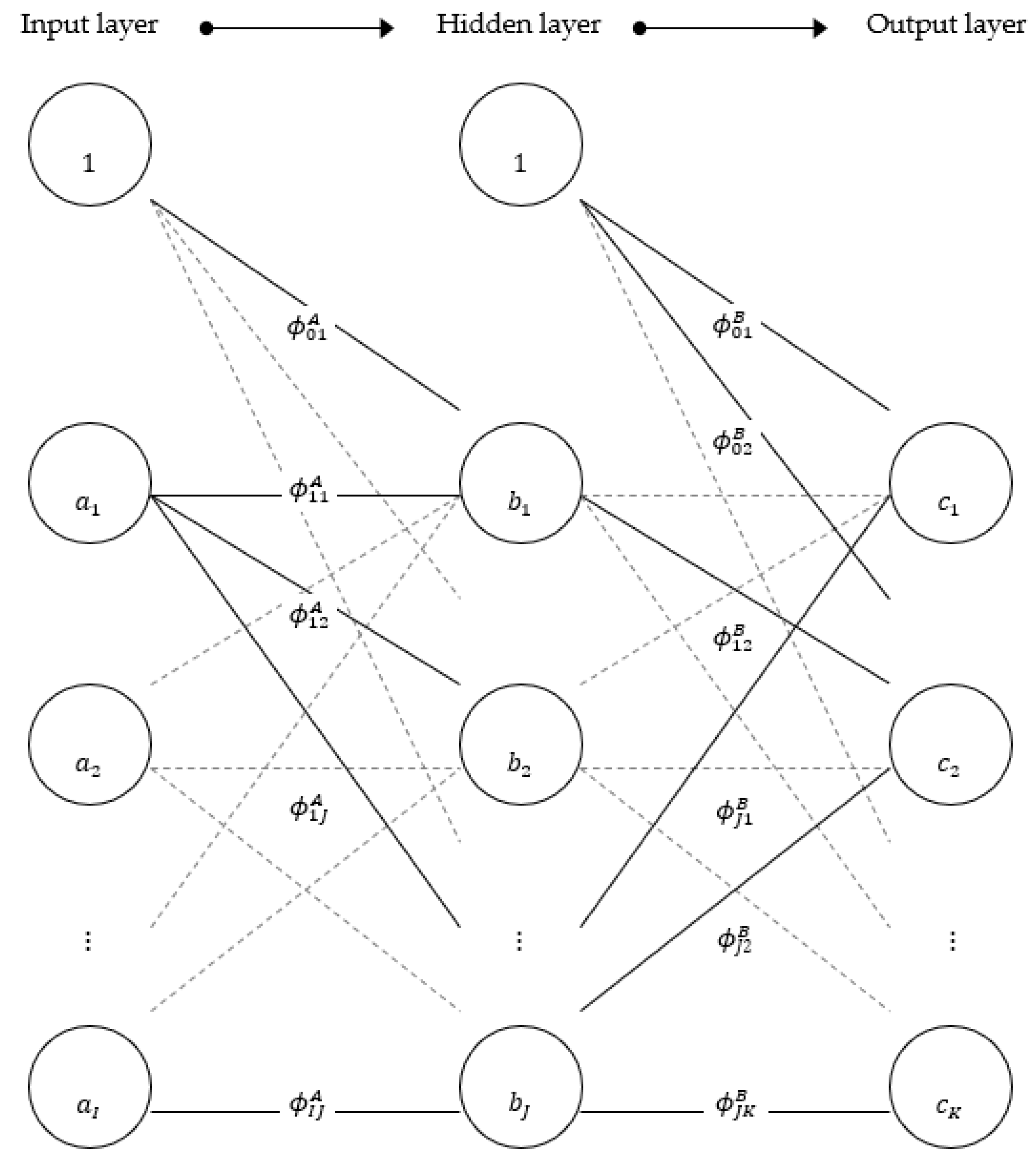
7.2. Artificial Neural Networks

An artificial neural network, or simply neural network or A N N , is a model inspired by the human nervous system. The human nervous system is a network of billions of neurons (nerve cells) in the human body. Each neuron is connected to a number of other neurons forming a very complex parallel system; the neurons interconnect and communicate by sending chemical signals between each other. Depending on the strength of each signal, a neuron transmits a signal if the aggregated signal from other neurons is strong enough.
The literature on A N N s is vast and there exists a wide range of different network structures, each with its own advantages and disadvantages. The most common one is the multilayer perceptron ( M L P ). Although an M L P network has a specific functional form, it is more flexible than traditional linear models. The main advantage is that M L P networks can approximate any non-linear continuous function [12]. A typical structure of an M L P network is presented in Figure 1. The network consists of an input layer, a hidden layer, and an output layer. The input layer consists of input nodes (similar to neurons in the human nervous system) that feed the network with relevant data. These data form a linear combination (weighted sum) and are sent to the hidden layer for activation. The weighted sum in each hidden node is activated using a transfer function that transforms the linear combination to fit into a pre-determined interval. The transformed sum is then weighted and sent to output nodes in the output layer.
The input nodes are naturally the part where values are admitted into the model:
A = a 1 a 2   a I
Connections between nodes are weighted and determine the relevance of the transfer signal from one node to another. These weights are typically randomized at the beginning of the training period and then adjusted using appropriate methods during training. The weights can be presented using matrix terminology. Consider an I × J matrix for the input/hidden weights and a J × K matrix for the hidden/output weights:
W A = ϕ 11 A ϕ 12 A ϕ 21 A ϕ 22 A ϕ 1 J A ϕ 2 J A ϕ I 1 A ϕ I 2 A ϕ I J A            and            W B = ϕ 11 B ϕ 12 B ϕ 21 B ϕ 22 B ϕ 1 K B ϕ 2 K B ϕ J 1 B ϕ J 2 B ϕ J K B
In addition, there is a bias node in the input layer and each hidden layer, which serves as a constant in the model and its value is equal to 1 at the beginning of the training period. The bias changes along with the weights throughout the training and corresponds to the constant coefficient in a standard regression. The bias weights are denoted ϕ 0 j A and ϕ 0 k B for the input and hidden layers, respectively.
The transfer function is located in each hidden node (and output node if necessary) and is normally of sigmoid type. A sigmoid function produces an s-shaped curve and is real-valued and differentiable, with either a non-negative or non-positive first derivative and exactly one inflection point. There are also two asymptotes for t ± . The logistic function produces a value inside the interval 0 , 1 . If the values used as input or desired output are in another region, it would be more reasonable to use another transfer function, such as the hyperbolic tangent, which produces values inside the interval 1 , 1 . The network’s training algorithm makes use of the first derivative of the transfer function. Because of the trivial deduction of their first derivative, the two functions mentioned above are the most commonly used transfer functions in neural network literature [14].
The logistic function and its first derivative:
f x = 1 1 + e x            f x = f x 1 f x
The hyperbolic tangent and its first derivative:
f x = e 2 x 1 e 2 x + 1            f x = 1 f x 2
Many neural network models use hard limit threshold functions that produce two or more values, depending on the node sum. An example of this is the binary function with a limit threshold τ . This function would yield 1 for x > τ and 0 for x τ :
The hidden nodes receive a weighted sum from the different input nodes plus the input bias, which is put through the transfer function:
B = b 1 b 2 b J         where     b j = f ϕ 0 j A + i = 1 I ϕ i j A a i       j = 1 , 2 , , J
The output node is the final destination of the transferred data. The output may be linear in the sense that the weighted sum from all the hidden nodes plus the bias term is considered the final output. Alternatively, one can use a transfer function in the output node to produce a value inside a desired interval. The output value for output node k is:
c k = f ϕ 0 k B + j = 1 J ϕ j k B f ϕ 0 j A + i = 1 I ϕ i j A a i         where             k = 1 , 2 , , K
For time series prediction, using one output node, lagged values of y t and, assuming residuals are additive white noise, the functional form would be:
y t = f ϕ 01 B + j = 1 J ϕ j 1 B f ϕ 0 j A + i = 1 I ϕ i j A y t i + ε t
A N N s possess strong parallel mapping skills. Acknowledging that, we also take note of the biggest disadvantage of A N N s: complexity increases exponentially with network size. One of the most important issues when constructing an A N N is to find a balance between precision and complexity.
When the architecture is set, the M L P network weights must be estimated. This process is called training. The most popular learning paradigm is the gradient descent algorithm, which is also called backpropagation [14]. The objective of the training algorithm is to minimize the mean square error ( M S E ) of the entire training set of data which is defined as:
M S E = 1 N n = 1 N k = 1 K e k n            where          e k n = 1 2 c k * c k 2
where M S E is the total error of all patterns presented to the model and k refers to the output node. c k is the actual output from the model and c k * is the desired output (what the model should have forecasted). e k n is the instantaneous error resulting from the difference between c k and c k * in output node k in training pattern n . This error is propagated backward through the network to allocate it to the right weights and adjust them using the following equations:
t ϕ j k B = η δ k b j + γ t 1 ϕ j k B       where       δ k = c k * b j f s k
t ϕ i j A = η δ j a i + γ t 1 ϕ i j A       where       δ j = k = 1 K δ k ϕ j k B f s j
The derivations of Equations (10) and (11) can be found in [9]. The δ k and δ j terms are the local gradients for the hidden layer and input layer. Gradients represent a sensitivity factor, determining the direction of the search in weight space for the optimal weight. η is called the learning rate and γ is called the momentum; both terms have values between zero and unity. The smaller we set η , the smaller the weight change is from one iteration to the next. The momentum term γ is added to increase the learning rate without destabilizing the network. We divided the data set into three parts, training set, validation set, and prediction set. One training iteration of the entire training set is called an epoch. Usually, thousands of epochs are needed to sufficiently modify the network weights.
With the use of multi-core processors and the Internet (here under cloud computing), computing is becoming more and more concurrent. Concurrent computing is computing where several computations are being executed at the same time. This is in contrast to sequential computing, where one computation is completed before the next starts.
Examples of concurrent computing are parallel computing (multi-core processors) and distributed computing (across the Internet). In parallel computing, a task is distributed over multiple processes that execute concurrently on separate processing cores and interact with each other to complete the task [15]. Distributed computing is computing where a task is distributed over multiple processes and the processes run on multiple computers. This makes communication between processes costly, time-consuming, and a potential security risk. The actor model is an architectural model for concurrent computation, hereby unifying parallel computing and distributed computing. The model was proposed by Carl Hewitt in 1977 [9].

8. The Actor Model

The actor model is a system built up of a collection of concurrent autonomous entities called actors. An actor is a computational entity that, in response to messages it receives, can respond concurrently. An actor is a computational entity that, in response to a message may concurrently send the messages to other actors, create new actors, and designate how to handle the next message it receives. There are three ways an actor can provide addresses to other actors: when the actor is created, through messages, and through addresses of the actors it has created [11].
The addresses of actors should be independent of the physical location of the actors. This means, there should be no difference in programming the communication with an actor running on the same processing core or a different computer in a network [12]. All communication is conducted by sending asynchronous and non-blocking messages. Because the messages are asynchronous, actors do not hold any system resources while sending or receiving messages. This is in contrast to systems where memory is shared, and processes are using locks and waiting for locks to be released.
By definition, actors have a mutable internal state that is not shared directly with other actors. Only the actor itself can update its internal state. The only event in the actor model is message arrival events. While there are no events, the actors are idle. This means, for the system to do anything, an external message is needed. This is called an external event [13]. The actor receiving the external message can thereby start a chain of events in the system.

Actors and Agents

Michael Wooldridge distinguishes between two general usages of the term agent: the weak and the strong agent. The weak notion of an agent is a hardware or software-based computer system that has the properties listed below:
  • Autonomy: agents operate without the direct intervention of humans orothers, and have some kind of control over their actions and internal state;
  • Social ability: agents interact with other agents (and possibly humans) via some kind of agent-communication language [15];
  • Reactivity: agents perceive their environment (which may be the physical world, a user via a graphical user interface, a collection of other agents, the Internet, or perhaps all of these combined) and respond in a timely fashion to changes that occur in it;
  • Pro-activeness: agents do not simply act in response to their environment. They are able to exhibit goal-directed behavior by taking initiative.
The strong notion of an agent includes the properties of the weak notion, but in addition, a strong agent uses concepts such as knowledge, belief, honesty, and commitments [15]. Actors and agents share some similarities with regard to autonomy and their ability to send messages. However, actors and agents have mostly different properties. Two of the most significant differences are:
  • Actors need to get a message to be able to do any computation, while agents can react to an environment or take the initiative.
  • Actors need the address of another actor in order to communicate (send messages). The notion of agent does not have this restriction.
The first difference means actors are passive in between processing messages. In contrast, agents can be continuously active by observing an environment. This environment can include other agents. The second difference means that communication between actors is carried out only through message passing, and for an actor to send a message to another actor the address is needed. While agents A and B may, for instance, communicate by letting agent A modify something in the environment that agent B is observing, agent B can then act upon observing certain conditions in the environment. The address of the agent is, therefore, not needed in this case.

9. Design and Development of the System

The platform consists of four independent parts: a data collector, a trading system runner, an application programming interface (REST API), and a web application. The reason for dividing the platform into these separate parts is to make it decoupled, so that each part can be exchanged without interacting with the other parts, making each part independently testable [16]. While testing, the other parts do not need to run and only database entries used by the tested part are needed. These database entries can be added manually to test certain functions and situations. The platform is not tied to a specific financial instrument.

The Data Collector

The task of the data collector is to collect historical trading data for a financial instrument, from an external source, and add it to the database. After all the data are collected, the data collector starts collecting live data. Multiple resulting database tables can be created of an arbitrary granularity, such as per trade (also called tick), minute, hour, and day. While the resulting database tables should be equal for all financial instruments, the interface to the source has to be source-specific. This is because, for the most part, there is no common way for accessing the data. Instead, each source usually has its own method of accessing data.

10. Artificial Neural Networks for Trading Systems

The methodology for the design and development of trading systems in this paper is based on the work of Bruce Vanstone and Gavin Finnie [17]. ANNs use supervised learning, and while ANNs differ in structure and output from trading system to trading system, the input variables are taken from a shared set of input variables.

10.1. Technical Indicators

The methodology for the design and development of trading systems in this paper is based on the work of Bruce Vanstone and Gavin Finnie, where ratio structure and oscillator indicators built from price and volume are used. This is because we want the ANN to handle the relative behavior of price and volume, not the exact value. A set of technical initiators is selected as possible input variables to ANNs. The indicators selected are indicators that are popular and have shown promising results regarding predictions of financial markets. The selected technical indicators are shown in Table 1. The indicators are computed from granulated data, not from tick data. In Table 1, n is an indicator of the number of prior time periods to consider in the calculation, k is some constant step size, Ct is the closing price at time t, Lt is the low price at time t, Ht is the high price at time t, LLn is the lowest low in the past n time periods, HHn is the highest high in the last n time periods, and MACn and MAVn are the price- and volume-moving averages for the last n time periods.
The different indicators are defined mathematically in Table 1. The stochastic %K measures if a financial instrument is overbought or oversold. If a financial instrument is overbought, it could indicate that the price is about to change. Momentum measures the momentum on the price change in an interval of fixed size. The Rate of Change measures the speed of the price change in the interval. William’s %R measures whether a financial instrument is overbought. The Accumulation/Distribution Oscillator is another indicator for price change. The Disparity Index measures the current price of a moving price average. The Price Oscillator and Volume Oscillator are used to compare a short-term average towards a long-term average, for the price and volume. The Aroon Oscillator is used to identify trends and trend strengths based on time periods since the highest high (DShn) and lowest low (DSln) are defined in a time window of n periods. The Relative Strength Index measures whether the stock is overshot or overbought based on the magnitude (Upt−1) versus the magnitude of losses (Dwt−1) over a specified time.
The Moving Average Convergence/Divergence is an indicator used to identify trends based on the difference between a fast- and slow-moving average.

10.2. Architecture

A Multilayer Perceptron Network (MLP) is used. The input layer has one neuron for each input variable, and the output layer has one neuron for each output variable. There are no standard rules for selecting the number of hidden layers and the number of neurons in each layer. The most common method for determining the appropriate architecture is experimentation with “trial-and-error”. A combination of literature review and experimentation are used to determine the number of hidden layers and the number of neurons in each layer.

10.3. Training

The ANNs are trained using a supervised backpropagation [12] training algorithm. The objective of the training is to change the weights so that the overall error in the mapping input of the training set to the corresponding target output is as small as possible. The overall error that we used is the root mean square (RMS) error function. This function maps the ANN’s current state into a point in the error space. The backpropagation consists of a feed-forward and a backward propagation phase. All the technical indicators used as input are scaled into the range [−1, 1]. The network goes through the two phases for every input/target pair in the training set. Going through the whole training set at one time is called an epoch.
An ANN is first initialized with random weights. All technical indicators are computed for each new data point and fed as input to the ANN. Trading is carried out according to the trading logic given in a NewTimePeriod function. After a number of data points are received, the ANN is trained on these new data points, thus defining the new market conditions [18].

10.4. Prediction of Trading Variables

Predicting the price of a financial instrument may seem to be an easy task to perform, but this has been shown to be difficult. The main reason is the amount of noise present in financial markets. This makes it hard for ANNs to find general patterns in price data. To reduce the noise in the data presented to ANNs, it has been proposed to use forward-looking technical indicators as output. Such technical indicators can be smoother and less exposed to noise, which can make them easier to predict. However, while the technical indicators might be predicted, this does not necessarily translate into a good trading system. This is because different technical indicators work on different markets and/or different market conditions.
ANN is used to predict technical indicators that are profitable on historical data. The training set consists of the 13 technical indicators from Table 1 computed for time t − 1 and t as input, where t is the time of the last data point. The corresponding output consists of the selected indicator computed for time t + 1. This means that there are 13 × 2 neurons in the input layer and only one neuron in the output layer. This means that input (t − 1, t) is mapped to output t + 1. The reason for only looking one period forward for the technical indicators is that the output indicator communicates nothing about the price change from the input time (t) to the output time (t + 1). Therefore, the selected output indicator is computed for time t and traded with precedence to the ANN output. In Table 1, the variables are computed for time t − 1 and t as input, where t is the time of the last data point. The corresponding output consists of the selected indicator computed for time t + 1, which is the indicator of one data point forward in the future. This means that there are 13 × 2 neurons in the input layer and one neuron in the output layer and input (t − 1, t) is mapped to output t + 1.

10.5. ANN Output

The different indicators tested as output for the ANN are ROC, %R, DI, and AO. The reason for selecting these indicators is that they have been shown to be profitable in all periods. The output is scaled to the same range as the input indicator of the same type. A modification of the first system may be conducted by the first trading system output variable proposed by Vanstone and Finnie in. The output variable measures the expected price movement. In [18], the authors suggest building a variable by measuring the maximum price change over a time interval after the input time. The size of the time period should be selected relative to the desired frequency of trades. This is in contrast to the prediction of technical indicators where prediction is always one period ahead:
OutUp(t) = (max(Ct +1, …, C t+n)−Ct)/Ct
where C is the vector of close prices, t is the index of the inputs that should result in OutUp(t), and n is the number of future time periods to be included in the calculations. This variable should, according to Bruce Vanstone and Gavin Finnie [17], result in a highly tradeable indicator on all market conditions. We may also suggest measuring the strength of a downward position as:
Outdown(t) = (min(Ct +1, …, Ct+n) − Ct)/Ct
Two separate ANNs were used for trading: one predicting OutUp(t) and one for Outdown(t). Both ANNs use the same input and architecture. In addition, a trading system is used for price direction by classifying the input into one of four classes. The input consists of all the technical indicators shown in Table 1, calculating for time t (13 inputs). The output of the ANNs is a vector of 4 elements corresponding to the following classes:
  • Two percent or more price increase, [2, ∞].
  • Zero to two percent price increase, (0, 2).
  • Zero to minus two percent price decrease, [−2, 0].
  • Two percent or more price decrease, (−∞, −2).
The numbering indicates their place in the output vector. All intervals are given in percent. The class with the highest degree of membership is declared as the winner. It is possible to have multiple winners. The ANN has four output neurons and each neuron represents a class. The output is a vector of four dimensions, indicating the membership input degree. The target output may be defined as a vector (1 0 0 0). This vector indicates that the target is increasing by two percent or more. The membership value is a real number and the class with the highest degree of membership is declared as the winner.
An alternative predictive output is the direction of the price. While this seems easier, research shows us that it is not easy to determine the strength of the change. For instance, a high degree of predicted price change does not necessarily indicate a large price change. An ANN will predict the direction of the price change from the current time (t) until the next time (t + 1). See Figure 2. The output consists of a value within the interval [−1,1]. The target output is:
  • 1 if the price change is positive, more than 2%;
  • 0 if the price change is less than 2% and positive;
  • −1 if the price change is negative, more than 2%.

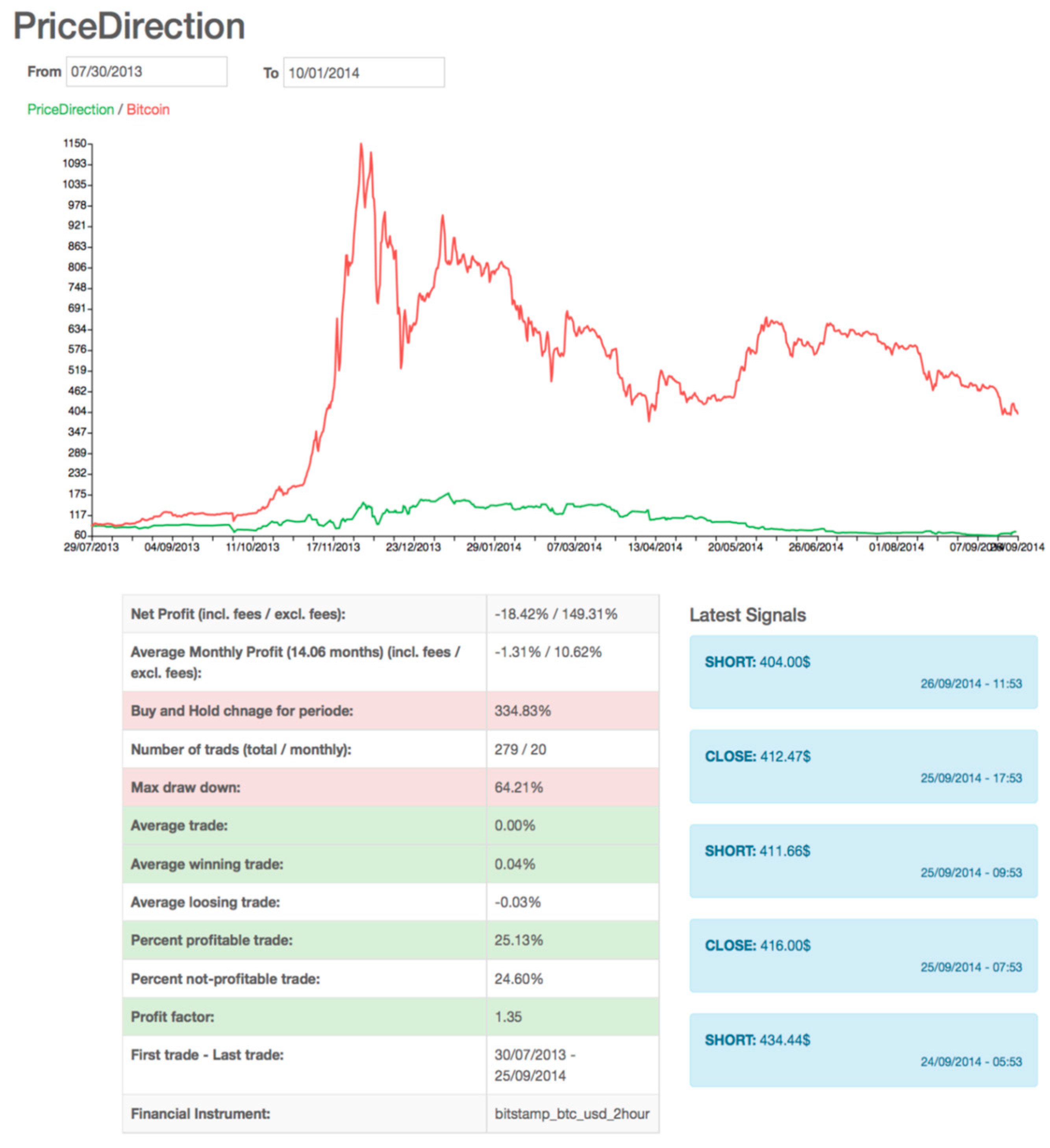
11. Experiments and Results

In order to backtest the proposed trading systems, some simple strategies were selected for money management and portfolio construction. For money management, an all-in approach was used. By this, we mean that when a position is signaled the position is taken with all available assets. Moreover, there is no need for portfolio construction because all trading systems are tested on only one financial instrument, bitcoin. Bitcoin data are taken from the Bitstamp exchange [7]. The trading systems are tested on two granularities, 2 h of data and one day of data. A separate test is carried out for each granularity. All trading is simulated by the use of market orders on the price used at last order before the time of input (t). This means that the spread is not included in the calculations and the real price could have varied a little. However, the trading systems proposed in this paper do not trade so frequently that the spread would have much impact on the results. The reason for not including the spread is because the data sets do not include information about the spread. However, the trading commission has a much greater impact on the results and is included.

Testing on the Bitcoin Market

The indicators were tested on data from the period from 30 July 2013 to 1 October 2014. The results of the whole period, 30 July 2013 to 1 January 2014 and 1 January 2014 to 1 October 2014, are reported. The bitcoin price in these periods went up 335%, up 682%, and down 44%, respectively. The reason for testing on these specific periods is to test the indicators on different market conditions. For every indicator, before a new position is taken, any old position is closed. The values of the indicator variables are set experimentally.
When the Rate Of Change (ROF) indicator rises above zero, a long position is taken, and when it falls below zero, a short position is taken. The William’s %R indicator has a range from 0 to 100 and is normally traded by taking a long position when the indicator is below 20 and taking a short position when the indicator is above 80. For the Disparity Index, a rise above zero is taken as a long position, and when it falls below zero, a short position is taken [8]. The Relative Strength Index indicator has a range from 0 to 100 and is normally traded by taking a long position when the indicator is below 30 and taking a short position when the indicator is above 70. When the Aroon Oscillator rises above zero, a long position is taken, and when it falls below zero, a short position is taken. The Moving Average Convergence/Divergence indicator consists of two moving averages, one slow and one quick. When the quick one crosses above the slow, a long position is taken, and when the quick one crosses below the slow, a long position is taken.
A trade is defined as the process of taking a position on the market and closing the position. This means that, for each trade, there are two transactions executed on the market. For each simulated transaction in the backtest a broker commission of 2% is used. Each trading system section consists of tables displaying the best-found trading system variable values and the corresponding results. The results focus on profits in some specific time periods, but other statistics are included in the discussion when appropriate. The backtest is conducted on the period from 30 July 2013 to 1 October 2014. The results of the whole period, 30 July 2013 to 1 January 2014 and 1 January 2014 to 1 October 2014, are reported. The bitcoin price in these periods went up 335%, up 682%, and down 44%, respectively. The reason for testing on these specific periods is to test the indicators on different market conditions.

12. Conclusions and Further Work

A platform for running, testing, and comparing trading systems was developed based on the actor model. Such a model uses small computer resources while waiting for new data points. The actor model makes it easy to conduct concurrent computations. For instance, if a trading system uses an ANN and the ANN needs to be retrained, the actual trading system does not need to be stopped in order to train the new ANN. The new ANN may be trained while using the old ANN. As soon as the new ANN is finished, the new ANN may replace the old ANN.
The framework Akka [19,20] was used to make it possible for the trading system runner to deploy new trading systems on separate JVMs, and also on other computers. This makes the platform very scalable. The design of the platform makes it decoupled and fault tolerant. The different parts of the platform only communicate through database entries by posting completed work to a database that is watched by another part of the system. If one part of the platform encounters an exception, that part is restarted and continues working it left off. No other part of the platform needs to take into account that an exception occurred. The platform also makes it possible to run and backtest all the trading systems at the same time. In the trading systems developed, both short and long positions are used.

Further Work

The trading systems presented in this paper should be tested on a larger amount of bitcoin data. This could be solved by using finer granularity data, but the volume of bitcoin is not very high compared with other financial instruments. Therefore, the best way to benchmark the trading systems is to wait for more data to be accumulated and run the trading systems on the new data. Another way for potential improvement is by selecting other values of the different variables. The variables of the trading systems could be optimized by using evolutionary computation methods [21,22,23]. However, to evaluate the fitness function of the trading system, the system has to be executed on historical data and, therefore, may vary for a very long time.
It could be interesting to test the trading systems on data of other financial instruments. This would only require the implementation of a new data collector. The system already has support for running multiple data collectors at the same time [24,25,26]. The system can also run trading systems using data from different financial instruments concurrently. This means that the system could be extended with parts for portfolio optimization and money management.

Author Contributions

Conceptualization, T.S.K.; Formal analysis, A.H.S.; Writing—original draft, T.S.K. and A.H.S. All authors have read and agreed to the published version of the manuscript.

Funding

This research received no external funding.

Conflicts of Interest

The authors declare no conflict of interest.

References

  1. Bianchi, D.; Born, A.; Di Benedetto, M.D.; Di Gennaro, S. Active Attitude Control of Ground Vehicles with Partially Unknown Model. IFAC PapersOnLine 2020, 53, 14420–14425. Available online: www.sciencedirect.com (accessed on 15 June 2023). [CrossRef]
  2. Box, G.; Jenkins, G. Time Series Analysis: Forecasting and Control; Holden-Day: Oakland, CA, USA, 1970. [Google Scholar]
  3. Bøvre, J.O.; Viervoll, P.K.; Kristensen, T. An Artificial Walk Down Wall Street: Can Intra-Day Stock Returns Be Predicted Using Artificial Neural Networks? In Proceedings of Eight International Conference on Perspectives in Business Informatics Research (BIR2009); Kristiansand Academic Press: Kristiansand, Sweden, 2009; ISBN 978-91-633-5509-7. [Google Scholar]
  4. Clinger, W.D. Foundations of Actor Semantics. 1981. Available online: http://dspace.mit.edu/handle/1721.1/6935 (accessed on 15 June 2023).
  5. NASDAQ. Nasdaq. February 2014. Available online: http://www.nasdaq.com/ (accessed on 15 June 2023).
  6. XE. August 2014. Available online: http://www.xe.com (accessed on 15 June 2023).
  7. Bitstamp. August 2014. Available online: http://www.bitstamp.com/ (accessed on 15 June 2023).
  8. Hewitt, C. Actor Model of Computation: Scalable Robust Information Systems. 2013. Available online: https://docs.google.com/open?id=0Bykigp0x1j92M0p6b0ZWWE9SS3Frb3loV3NKX2sxdw (accessed on 15 June 2023).
  9. Hewitt, C. What Is Computation? Actor Model versus Turing’s Model. In Understanding and Exploring Nature as Computation; World Scientific: Singapore, 2012. [Google Scholar]
  10. Engelbrecht, A.P. Computational Intelligence: An Introduction; John Wiley and Sons: Hoboken, UK, 2007; ISBN 0470035617. [Google Scholar]
  11. Gul, A.A.; Wooyoung, K. A unifying model for parallel and distributed computing. J. Syst. Archit. 1999, 45, 1263–1277. Available online: http://www.sciencedirect.com/science/artickle/pii/S1383762198000678 (accessed on 15 June 2023).
  12. Chen, S.H.; Wang, P.P. Computational Intelligence in Economics and Finance; Springer: Berlin/Heidelberg, Germany, 2004; ISBN 978-3-642-07902-3. [Google Scholar]
  13. Grøtte, O. Original Norwegian Title: Aksjekjøp og Datatrading: Metode, Psykologi, Risiko og Strategier. English Title: Stock Purchases and Daytrading: Methodology, Psychology, Risk and Strategies; Hegnar Media: Oslo, Norway, 2006; ISBN 9788271460310. [Google Scholar]
  14. Kristensen, T. Original Norwegian Title: Nevrale Nettverk, Fuzzy Logikk og Genetiske Algoritmer. English Title: Neural Networks, Fuzzy Logic and Genetic Algorithms; Cappelen Akademic Publisher: Oslo, Norway, 1997; ISBN 82-456-0203-5. [Google Scholar]
  15. Wooldridge, M.; Jennings, N.R. Intelligent Agents: Theory and practice. Knowl. Eng. Rev. 1995, 10, 115–152. [Google Scholar] [CrossRef]
  16. Tomasini, E.; Jaekle, U. Trading Systems: A New Approach to System Development and Portfolio Optimization; Harriman House Series; Harriman House: Harriman House, UK, 2009; ISBN 9780857191496. [Google Scholar]
  17. Vanstone, B.; Finnie, G. An empirical methodology for developing stockmarket traiding systems using artificial neural networks. Expert Syst. Appl. 2009, 36 Pt 2, 6668–6680. Available online: http://www.scienencedirect.com/science/article/pii/SO957417408005836 (accessed on 15 June 2023). [CrossRef]
  18. Heaton Research Inc. Encog Machine Learning Framework. September 2014. Available online: http://www.heatonresearch.com/encog (accessed on 15 June 2023).
  19. Karmani, R.K.; Shali, A.; Agha, G. Actor Frameworks for the JVM Platform: A Comparative Analysis. In Proceedings of the 7th International Conference on Principles and Practice of Programming in Java, Calgary, AB, Canada, 27 August 2009; pp. 11–20. [Google Scholar]
  20. ypesafe Inc. Akka. February 2014. Available online: http://ww.akka.io (accessed on 15 June 2023).
  21. Mcadam, P.; McNelis, P. Forecasting Inflation with Thick Models and Neural Networks; Economic Modeling; Elsevier: Amsterdam, The Netherlands, 2005; Volume 22, pp. 848–867. [Google Scholar]
  22. Mills, T.C.; Markellos, R.N. Nonlinear Times Series in Financial Economics; Encyclopedia of Complexity and Systems Science; Springer: Berlin/Heidelberg, Germany, 2008. [Google Scholar]
  23. Nourani, E.; Rahmani, A.; Mand Navin, A.H. Forcasting stock prices using a hybride Artificial Bee Colony based neural network. In Proceedings of the 2012 International Conference on Innovation Management and Technology Research, Malacca, Malaysia, 21–22 May 2012; pp. 486–490. Available online: http:////ieexplore.ieee.org&lpdocs/epic03/wrapper.htm?arnumber=6236444 (accessed on 15 June 2023).
  24. Rumelhart, D.E.; McClelland, J.L. Parallel Distributed Processing: Explorations in the Microstructure of Cognition; MIT Press: Cambridge, MA, USA, 1986. [Google Scholar]
  25. Shoham, Y. Agent-oriented programming. Artif. Intell. 1993, 60, 51–92. [Google Scholar] [CrossRef]
  26. Zhai, Y.; Hsu, A.; Halgmuge, S. Combining news and technical indicators in daily stock price trends prediction. In Proceedings of the 4th International Symposium on Neural Networks: Advances in Neural Networks, Part III, ISNN 07, Nanjing, China, 3–7 June 2007; Springer: Berlin/Heidelberg, Germany, 2007; pp. 1087–1096, ISBN 978-3-540-72394-3. [Google Scholar]
Figure 1. Graphical interpretation of a general three-layer perceptron where the arrows show the way information flows through the network. The input values are transferred (weighted) through a function, ƒ, in the hidden layer and subsequently transferred (weighted) to the output layer as the model output.
Automation 04 00014 g001
Figure 2. A trading system with two hours of data granularity. The graph of the trading system stops at the last trade.
Automation 04 00014 g002
Table 1. Technical indicators used as input to the ANN.
Indicator NameFormula
Stochastic %K (%K) % K t = C t L L n H H n L L n × 100
Stochastic %D (%D) % D t = i = 0 n 1 % K t 1 n
Stochastic slow %D (slow %D) S l o w % D t = i = 0 n 1 % D t 1 n
Momentum (MO) M O t = C t C t k
Rate of Change (ROC) R O C t = C t C t k C t k
Willlama’s %R (%R) % R t = H H n C t H H n L L n × 100
Accumulation/Distribution Oscillator (ADO) A D t = H t C t 1 H t L t
Disparity Index (DI) D I t = C t M A C n M A C n × 100
Price Oscillator (PO) P O t = M A C n f a s t M A C n s l o w M A C n f a s t
Volume Oscillator (VO) V O t = M A V n s m a l l M A V n b i g M A V n s m a l l
Aroon Oscillator (AO) A O t = ( n D S h n / n × 100 ( n D S l n / n × 100
Relative Strength Index (RSI) R S I t = 100 100 1 + i = 0 n 1 U p t i / n / i = 0 n 1 D w t i / n
Moving Average Convergence/Divergence (MACD) M A C D t = M A C n f a s t M A C n s l o w
Disclaimer/Publisher’s Note: The statements, opinions and data contained in all publications are solely those of the individual author(s) and contributor(s) and not of MDPI and/or the editor(s). MDPI and/or the editor(s) disclaim responsibility for any injury to people or property resulting from any ideas, methods, instructions or products referred to in the content.

