1. Introduction
Currently, research in the field of industrial robot control is focused on adding external sensors combined with advanced control strategies so that robots can work in unknown or semi-structured environments, thus, increasing the field of applications. Among the most widely used external sensors, vision sensors provide rich information about the working space. For this reason, vision-based control systems applied to robotics have been extensively studied in recent years.
Servo-visual control systems can be classified into image- or position-based systems according to how the control errors are defined, and in handheld or fixed camera system depending on the location of the vision camera with respect to the robot [
1]. Furthermore, these control systems can be dynamic [
2] or kinematic [
3] depending on whether or not the dynamics of the robot are considered in its design.
Although the parameters of the models of these control systems can be obtained with sufficient precision through calibrations or identification techniques, there will always be uncertainties due to assembly errors, variations in the load handled, etc. To deal with these uncertainties, various adaptive robot controllers have been proposed. In [
4], uncertainties in the kinematic parameters of a handheld camera system were considered, without demonstrations of the stability of the system. In [
2], only the uncertainties in the parameters of the vision system were dealt with, and local stability results were presented. On the other hand, in [
5], a precise knowledge of the kinematics of the robot and the vision system was assumed, considering only uncertainties in the robot’s dynamics.
The authors in [
6,
7,
8] presented adaptive controllers with uncertainties in the vision system with a proof of global convergence to zero of the control errors for positioning tasks and only with bounded errors for the following tasks. These works did not consider the dynamics of the robot. Other works, such as [
9,
10], considered uncertainties in both the camera and robot parameters for a fixed camera system: the first with the assumption of needing an explicit measurement of the speed of the end of the robot in the image, and the second with a similar approach to the first but that avoided this measurement.
Both works dealt separately with the problem of adapting the parameters of the camera and the robot with a cascade structure and with a complete stability test of the system. Although the design of the adaptive robot controller followed a classical structure, it was based on a model with torque and force inputs, which is not the case with a real industrial robot. The design of the servo-visual controller was complex, and the simulation results did not effectively show a convergence to zero of the control errors. In the above mentioned works, the controllers were designed for planar or 2-D robots.
Currently, few works have considered adaptive servo-visual control for a 3-D robot. In [
11], an adaptive dynamic controller designed with backstepping techniques was presented that considered uncertainties in both the camera and robot parameters in a unified structure and allowed the tracking of objects in an asymptotic way. However, this was achieved due to the use of two fixed cameras mounted on perpendicular planes. In [
12], the author proposed an adaptive kinematic controller based on linearization techniques using a fixed camera. He considered two decoupled systems for the controller design, one for depth control and one for 2-D displacement control.
In [
13], an adaptive visual servo controller for trajectory tracking was presented using a calibrated Kinect camera, which acted as a dense stereo sensor, and a controller based only on the inverse kinematic model of the manipulator with a position-based control law. The authors did not provide a stability analysis of the proposed system, and the performance of the controller was verified through experimental results considering only the Root Mean Squared Error (RMSE) of the position of the robot end effector as representative of the controller’s precision.
In [
14], an adaptive control approach was presented considering the unknown robot’s kinematics and dynamics. The system used a calibrated camera to identify and calculate the Cartesian position of the robot’s operating end, on which an unknown tool was mounted, in order to estimate the 3-D dimensional information of the tool through the kinematic observer. The adaptive controller was of the free–model type combined with a kinematic observer. The stability of the closed-loop system was demonstrated by Lyapunov but was strongly conditioned to the convergence of the kinematic observer, which necessarily required persistently exciting trajectories to converge. The performance was shown through simulations.
In the work [
15], an adaptive controller for trajectory tracking by a 3-degrees of freedom (DOF) manipulator robot with a fixed camera configuration was presented, considering both the parameters of the camera as well as the dynamics of the manipulator and the dynamics of its electric actuators as unknown. They proposed a control system with two control laws based on the backstepping technique and with speed measurement in the image plane. The first control law set the armature current of the motors as an auxiliary control variable, and another control law was given to generate the voltage references to the motors as a final control action.
For the adaptation of the different parameters, eight adaptive laws were required, and they demonstrated the stability of the proposed closed–loop system proposed by Lyapunov’s theory, assuming that the estimated parameters did not cause a singularity in the estimation of the independent-depth image Jacobian matrix. The simulation results only showed the convergence to zero of the position and speed control errors in the image for a single circular path in the image plane, and they did not show the convergence of the estimated parameters or the auxiliary control variable and the articular positions of the manipulator during the task.
A similar approach was presented in [
16]; however, they avoided measuring the velocity in the image plane by incorporating a kinematic observer in cascade with the adaptive controller. They showed that the image space tracking errors converged to zero using a depth-dependent quasi-Lyapunov function plus the Lyapunov-like standard function and the asymptotic convergence of the observation errors in the image space. However their simulation results only showed the convergence to zero of the position control errors for a single circular path in the image plane. Similar to the previous work, they did not show the convergence of the estimated parameters, and, in addition, their results showed that the depth estimation error did not converge.
In [
17], a research work prior to the current one was presented, in which only a planar robot with two degrees of freedom was considered and where the unknown depth of the target was constant. In the present work, we propose an adaptive control system consisting of two cascaded controllers to control a 3-D robot. The first is an adaptive image based kinematic visual servo controller in a fixed camera setup, the aim of which is that the robot follows a desired 3-D Cartesian trajectory even without knowing the depth and relative orientation between the end of the robot and the camera.
The second controller is an adaptive dynamic controller, with joint velocity reference inputs from the first controller, which compensates for the dynamics of the manipulator even with uncertainties in its dynamic parameters. The designed control system considers the real dynamics of a Scara 3-D industrial manipulator robot, and the ultimately boundedness of the control errors of the entire system is demonstrated using Lyapunov’s theory. The performance is shown through representative simulations.
3. Simulated Experimental Platform and Vision System
To validate the proposed control system, we used the model of an experimental platform, which is a real SCARA Bosch SR-800 industrial robot of 4 DOF, available in our workplace and which represents a common robotic structure referred to in many works [
19].
The camera used in the experiments was a Drangonfly Express IEEE1394b camera. This camera is capable of acquiring and transmitting color images through the bus IEEE-1394b at a speed of 200 fps (frames per seconds) and with a resolution of 640 × 480 px (pixels). The camera should be mounted at a certain height over the manipulator robot in such a way that it allows for capturing the entire workspace. The images captured by the camera were processed in real time using functions from the OpenCV library to extract two characteristic points fixed to the end effector of the robot, which were used as image features in the visual servoing algorithm as explained below.
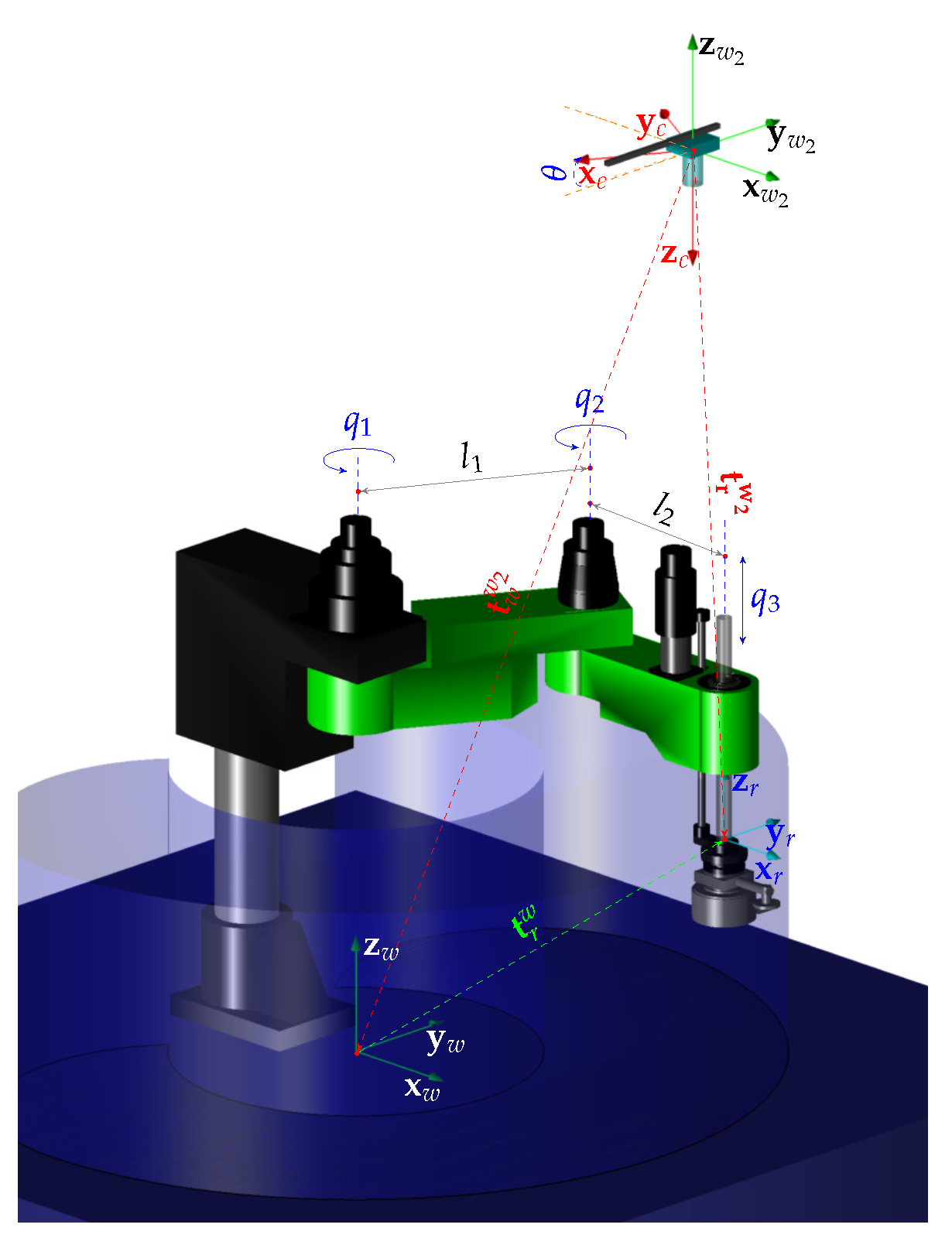
The modeling of the vision system provides the equations that relate the position of the end of the robot
and the fixed distance
to a second point, displaced on the
x axis of the robot frame
, in 3-D space with its corresponding projection on the image plane.
Figure 1 shows the frames associated to the manipulator
, the camera
, and the 3-D space
and
, to which the poses of the robot and the camera, respectively, are defined. The transformations between the inertial frames
and
, and between the frames
and
, are given by:
where
is the position vector (generally it is unknown) from
expressed in
and
with:
The 3-D point that represents the position of the robot is mapped to the point
of the camera image plane using:
where
is the point
expressed in homogeneous coordinates,
and
are the matrices of intrinsic parameters of the camera and of perspective projection,
is the robot position expressed in
, and
is an unknown scale factor. Operating algebraically, the expression (
7) can be rewritten in non-homogeneous coordinates as:
where
and
is the unknown depth of the operating end in the image frame
,
is the scale factor, and
is the coordinate vector of the center of the image (parameters of
). Similarly, the second point
on the end of the robot with
is mapped to the point
:
The distance between the two points in the image plane is given by
. Then, the vector of image features is defined as:
and its time derivative is given by:
where
,
is the Jacobian of the robot, and
represents the generally unknown parameters of the vision system.
5. Dynamic Compensation Design
This section ignores the perfect velocity tracking assumption considering a velocity tracking error (
) due to the dynamics of the robot. Under this condition, the closed-loop Equation (
23) now results in:
and the time derivative of (
24) is:
From (
28), outside the ball,
it is verified that
. Then, the control error is finally bounded by the value of
. Note that
does not necessarily converge to zero, since, by including the robot dynamics, the convergence of
is not always achieved as an attempt is made to identify a different structure for which the kinematic controller was designed. As a consequence, the control error increases.
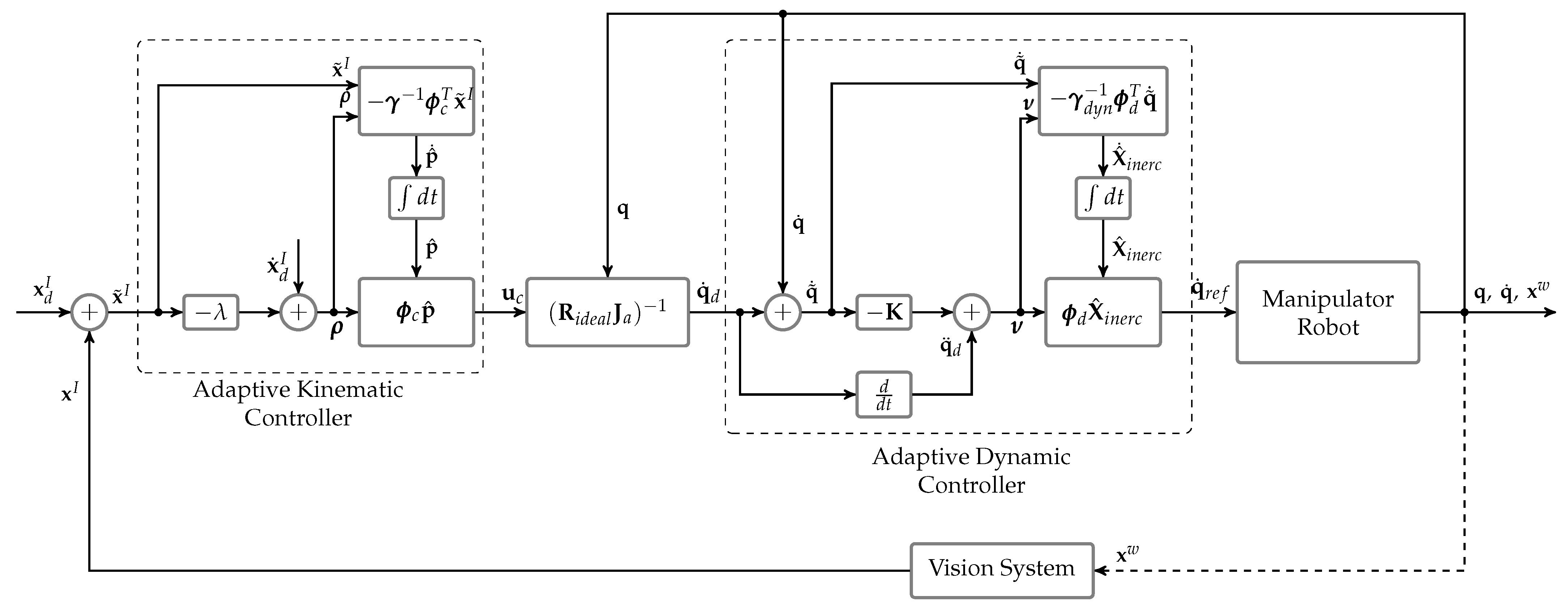
To solve the degradation of the kinematic control, a cascaded adaptive dynamic controller is proposed that makes the robot reach the reference speed provided by the kinematic controller, again restoring the good performance of the control system, see
Figure 2. Defining the speed control error as
, the following control law is proposed:
where
,
is a positive definite gain matrix,
represents the estimated robot parameters,
is the parameter error vector, and
and
are the matrices of inertia and Coriolis torques calculated with the estimated parameters. Replacing
in the dynamic model (
3), we obtain the closed-loop equation of the system:
We consider the following positive definite function:
and its time derivative in the trajectories of the system:
where the term
is zero, since
is the antisymmetric matrix calculated with the Christoffel terms. Defining, as adaptation law,
and replacing it in expression (
33), we obtain:
and therefore
and
. Furthermore, by integrating
over
, it can be shown that
. From expression (
31), it is proven that
. Then, by Barbalat’s lemma, we conclude that
with
, thus, achieving the control objective.
As proven above, the result
with
implies that:
Then, going back to Equation (
29) and introducing the convergence condition on
(
36), the error bound conditions of Equation (
26) and, therefore, the stability conditions previously obtained for the kinematic controller are asymptotically recovered even in the presence of unknown robot dynamics.
6. Simulations
In this section, we show simulation experiments that can be considered realistic and whose results are very close to those that would be obtained with the real robot. This is because the model used in these simulations is an identified model of the real robot, which represents the dynamics of both the rigid body and that of the electric motors and reduction gears in its actuators. A complete study of this model, the reduction of the total set of dynamic parameters to a minimum base parameters set that considers only the dominant and identifiable dynamics, and its subsequent expansion to model and identify the dynamics of its actuators is found in [
18].
To verify the performance of the proposed control system, realistic simulations were carried out for a positioning task and for a trajectory following task using the identified kinematic and dynamic model corresponding to the Bosch SR800 SCARA industrial robot. The parameters of the vision system were and px/mm, and errors of and were considered, respectively.
Figure 3 shows the evolution of the image characteristics for a positioning task, starting from rest at the position
and reaching the desired position
. The kinematic controller was applied first to the kinematic model of the robot, and then its dynamics were incorporated. The gains set to the values shown in
Table 1.
Figure 4 and
Figure 5 show the norm of the control error and the convergence of the vision system parameters; observing that, in both cases, the control error converged close to zero as indicated in the remarks of
Section 4.
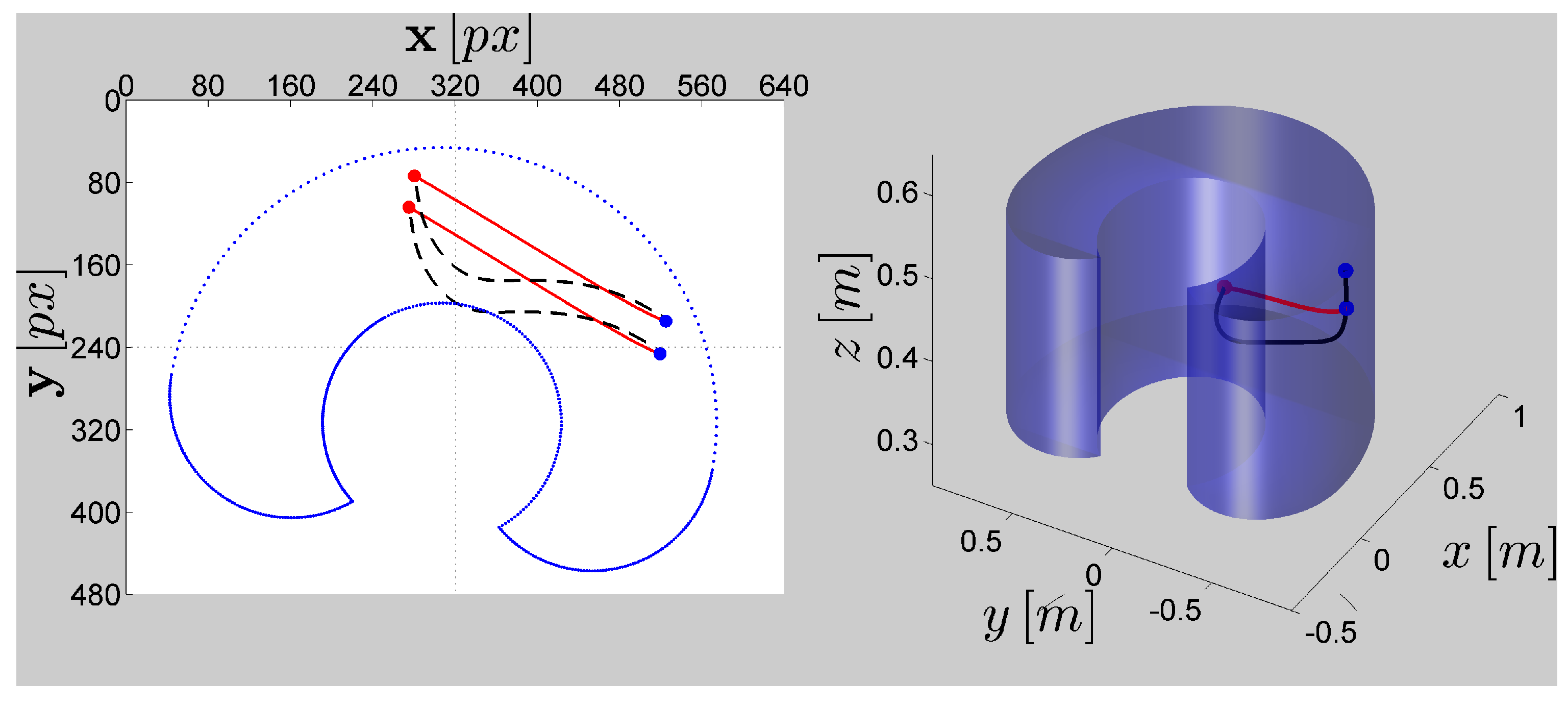
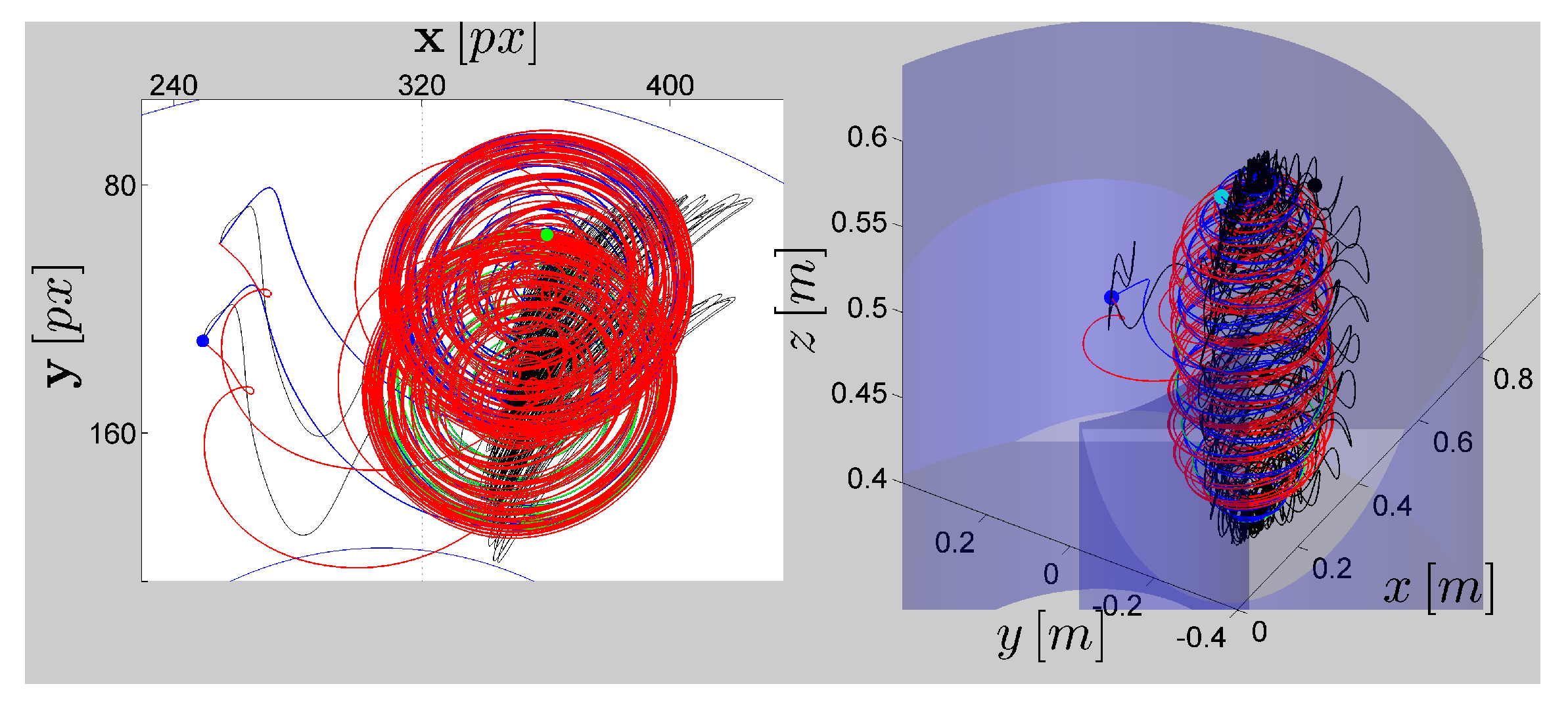
On the other hand,
Figure 6 shows the image feature vector
for the following task, starting from the position
and following a circular spiral reference
. The servo-visual controller was applied to a kinematically modeled robot, then the robot dynamics were incorporated, and later this dynamic was compensated with the adaptive controller, considering a
error in the robot parameters. The gains used in these three cases are shown in
Table 2.
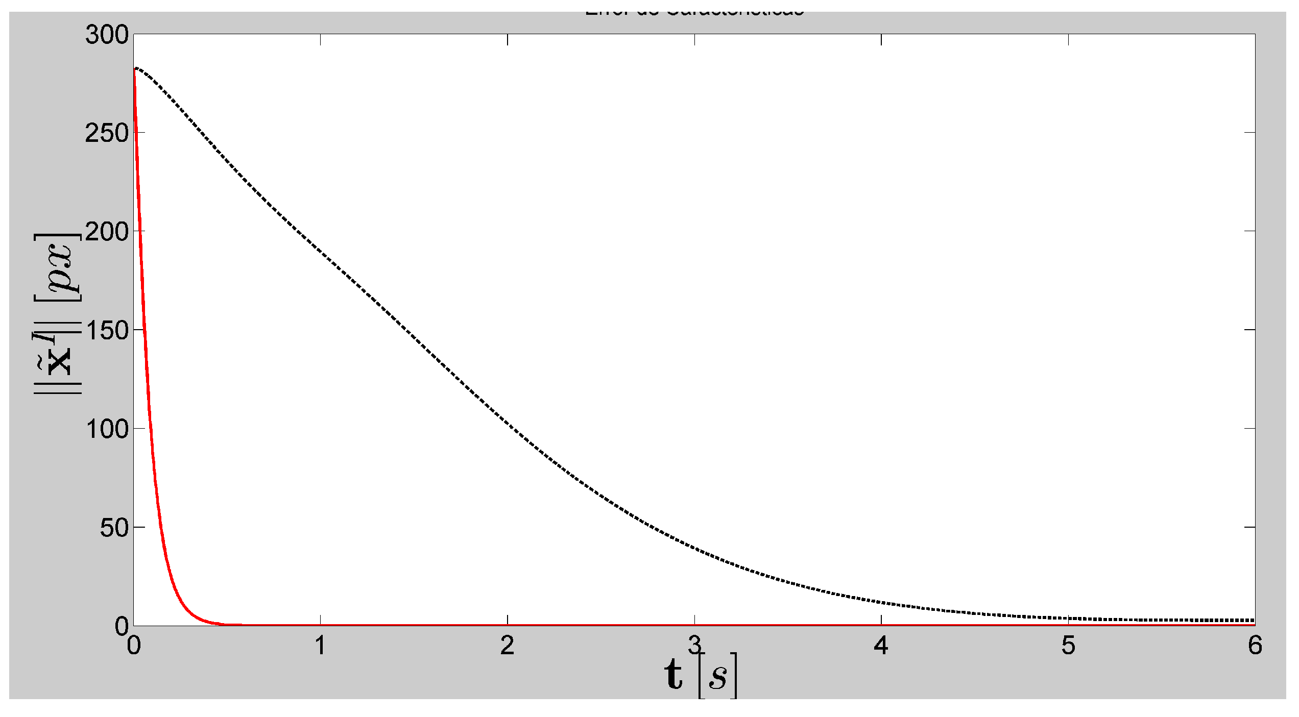
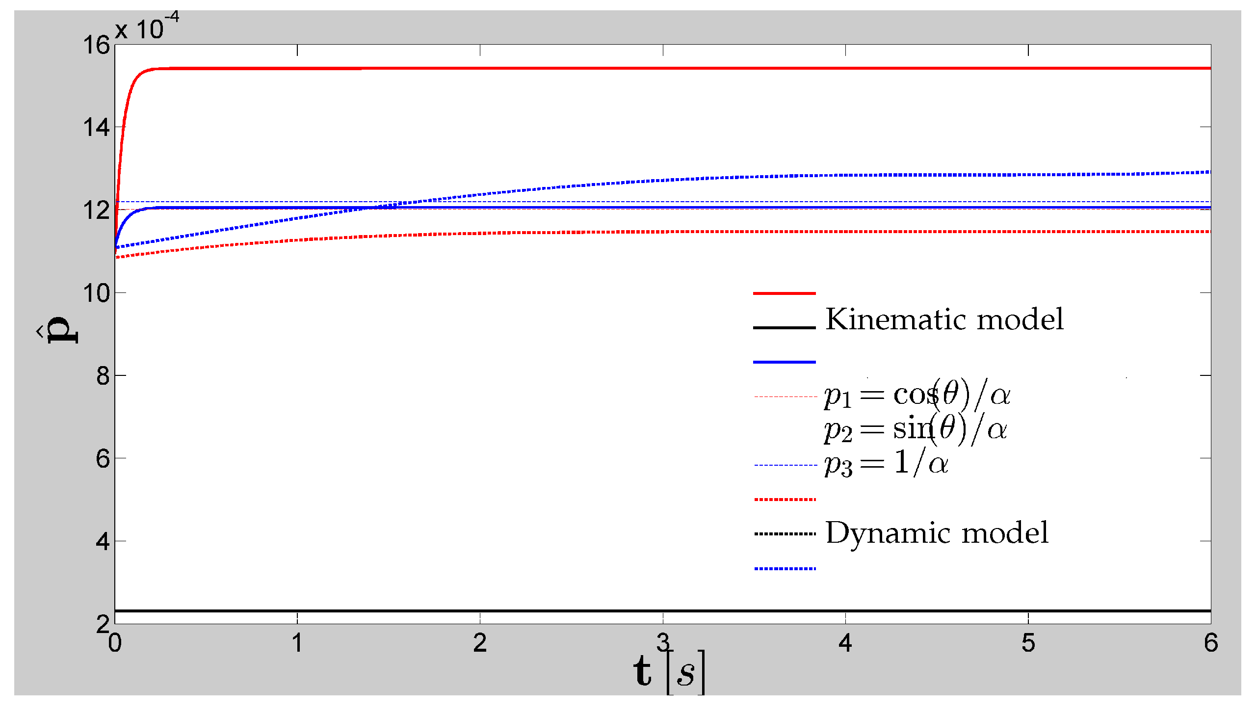
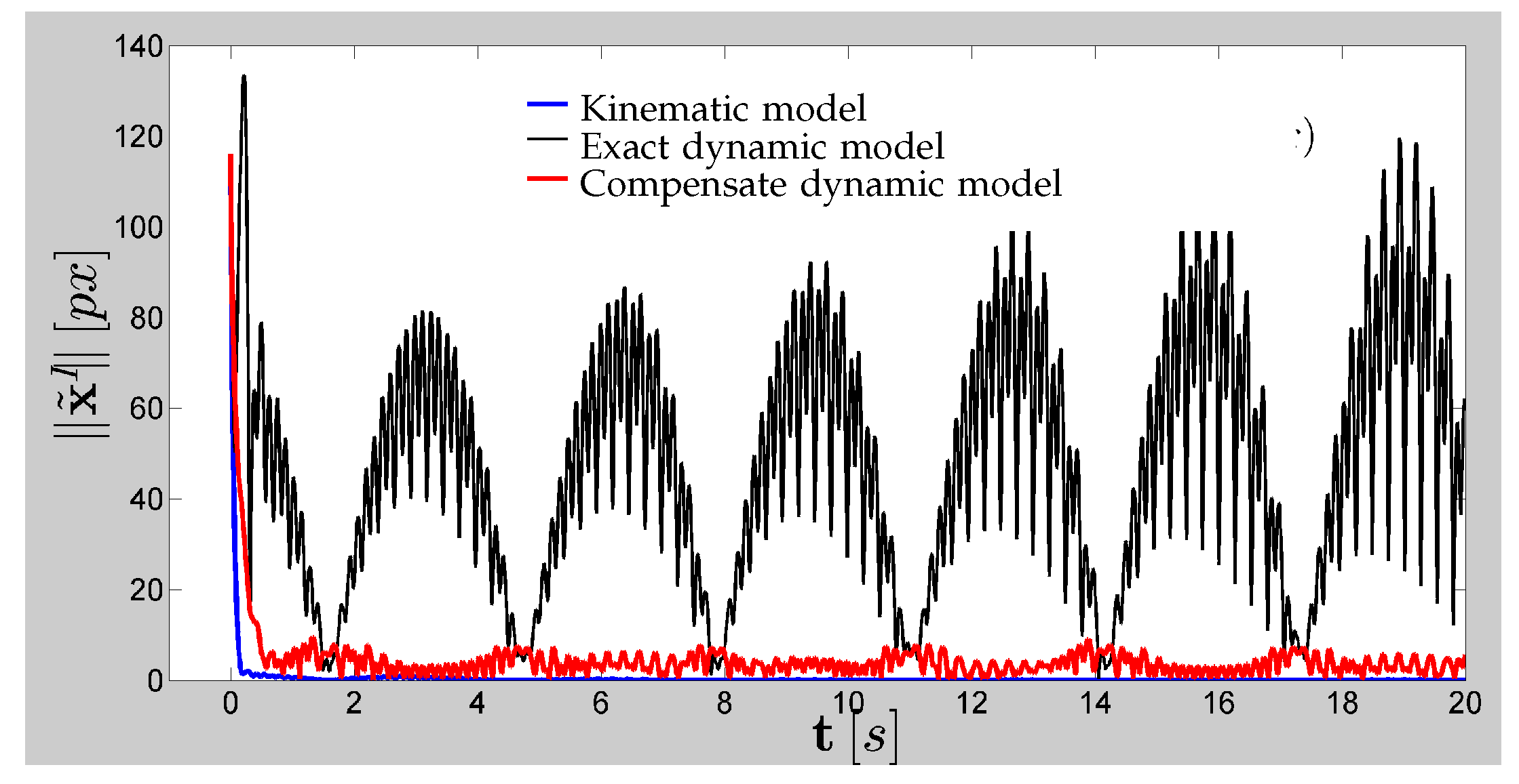
Figure 7 and
Figure 8 show the norm of the
vector and the convergence of the vision system parameters.
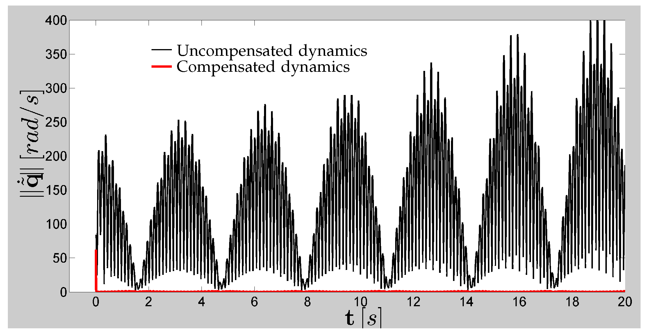
Figure 9 and
Figure 10 show the norm of the speed control error of the adaptive dynamic controller and the convergence of the dynamic parameters of the robot, respectively.
7. Discussion
In
Section 4, the design of two new adaptive servo-visual kinematic controllers for trajectory tracking with a 3-DOF manipulator robot was presented. The main contribution of these new control schemes is their simple design, their image-based control law, and their unique adaptation law, unlike previous works with complex controllers as in [
15,
16]. From a practical point of view, these do not require the measurement of speed in the image plane.
Finally, these schemes represent a generalization of previous work [
17] to the case of 3-D movement by the manipulator. This makes it possible to consider not only the intrinsic and extrinsic parameters of the vision system as unknown but also the depth of the objective, which can be time-variant and, as shown in
Section 3, can be estimated with an appropriate selection of the image characteristics.
In the simulations, the tracking task and the target points in the positioning task were chosen to show, in both cases, the performance of the controller without speed measurement in the case where the depth of the target is time-variant. It was also demonstrated by Lyapunov’s theory that the scheme that required a speed measurement of the image characteristics achieved an asymptotic convergence of the control errors in both the positioning and tracking tasks.
On the other hand, the scheme that did not require such measurement achieved an asymptotic convergence only in positioning tasks as shown by the simulation results of
Figure 4 and in following tasks in which the trajectories to follow sufficiently excited the dynamics of the system with the spiral trajectory whose result is shown in
Figure 7. However, in this last scheme, the stability analysis showed that, even in trajectories that were not persistently exciting, the control errors always remained bounded. In a previous work [
17], it was shown that, for the case of 2-D motion where the depth of the target was constant, the controllers always reached the control target even on non-exciting trajectories, such as a ramp type.
Figure 5 shows that the control actions generated by the kinematic controller, regardless of whether they applied to an idealized robot modeled only with its kinematics or to a real robot modeled with its exact dynamic model, the estimated parameters always converged on the positioning tasks, although not to the true values. This shows that, for these tasks, the performance of the kinematic controller is sufficient, and dynamics compensation is not required.
However, in high-speed tracking tasks that excite the manipulator dynamics, such as those in
Figure 6, it can be seen in
Figure 7 how the control error in the image plane converged asymptotically to zero when the control actions generated by the kinematic controller were applied to an idealized robot modeled only with its kinematics, and the estimated parameters converged to their true values as shown in
Figure 8. However, when these actions were applied to a real robot modeled with its exact dynamic model, the performance was very poor since it was attempting to control a system with a different structure than that for which the controller was designed, generating undesirable high frequency movements, like those shown in
Figure 8 and
Figure 9, and even the estimated parameters may not converge as can be seen in
Figure 8.
Figure 7 and
Figure 9 show that the performance of the kinematic controller is practically recovered when the manipulator dynamics were compensated, limiting the control errors as indicated by the stability test of the dynamic compensator in
Section 5, even with unknown manipulator parameters.
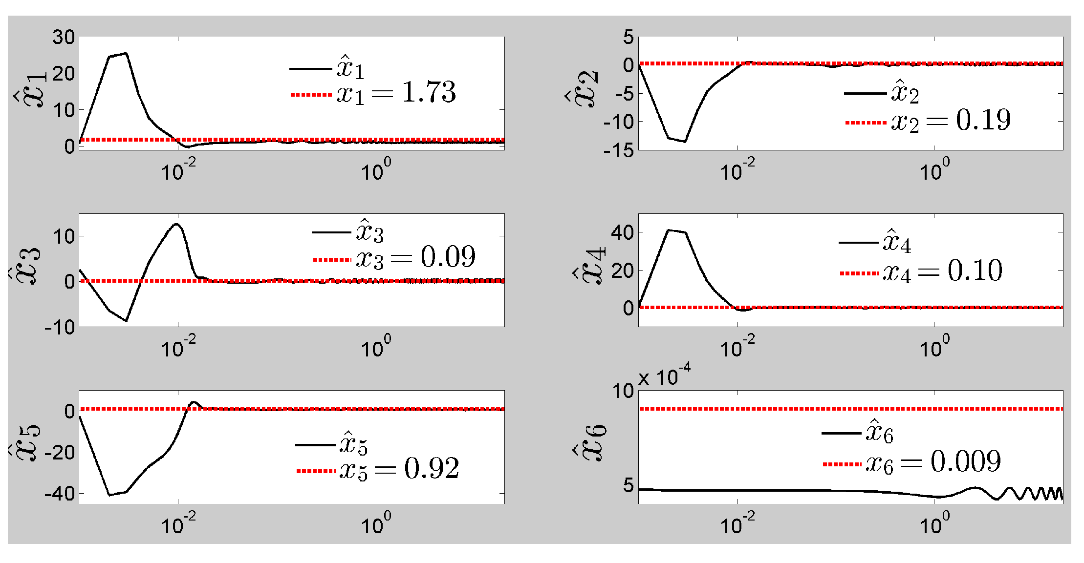
Figure 10 shows that most of the parameters converged to their true value and others remained bounded very close to them. Furthermore,
Figure 8 shows how the convergence of the vision system parameters was also recovered, although not to the true values as in the ideal kinematic situation.


