Article

Dual Data Streaming on Tropospheric Communication Links Based on the Determination of Beam Pointing Dynamics Using a Modified Ray-Based Channel Model

1
Electrical Cluster, School of Engineering, UPES, Dehradun 248007, Uttarakhand, India
2
Former Scientist ‘H’, Defence Electronics Application Laboratory, Dehradun 284001, Uttarakhand, India
3
Department of Electronics and Communication Engineering, Jawaharlal Nehru Government Engineering College, Sundernagar 175018, Himachal Pradesh, India
*
Author to whom correspondence should be addressed.
Telecom 2024, 5(1), 176-197; https://doi.org/10.3390/telecom5010009
Submission received: 12 December 2023 / Revised: 26 January 2024 / Accepted: 6 February 2024 / Published: 16 February 2024

Abstract

:
Tropospheric systems are widely used by military forces as they provide long-distance, real-time communication. Slow-fading propagation loss reduces link availability and limits its data-carrying capacity. Beam pointing dynamics provides knowledge of favorable heights at different times of the day in different seasons and a useful steering range. Beam steering, based on the beam pointing dynamics of the link, can overcome slow fading. The main contributions of this paper are the derivation of a realistic and accurate tropospheric channel model obtained by making important modifications to Dinc’s ray-based model. This paper also presents a method for determining beam pointing dynamics using the modified model. Beam pointing dynamics for two different links located in India have been determined in this paper using real-world data obtained from the Indian Meteorological Department. Another significant contribution of the paper is presenting the prospect of dual data streaming on tropospheric links using a fixed beam and a dynamically steered beam, based on the examination of beam pointing dynamics obtained for the two links. The main result presented in this paper is the comparison of powers received from the most favorable heights in a steerable beam system with the powers received in conventional fixed-beam systems for different days of the year. It has been shown that a higher received power can be achieved with beam steering. Another important result shown is the comparison of the achievable data rates for a single fixed-beam system and a dual-beam (one fixed beam and one dynamically steered beam) system. It has been shown that almost double the data rate is achievable in a dual-beam system. The method for the determination of beam pointing dynamics and the possibility of dual data streaming presented in this paper can significantly enhance the availability and capacity of tropospheric links.

1. Introduction

Tropospheric communication systems use the inhomogeneous nature of the troposphere for the propagation of radio frequencies beyond the horizon over distances as large as a few hundred kilometers. The volume of the tropospheric region enclosed by the intersection of transmit and receive antenna beams is known as the common volume. Tropospheric inhomogeneities present in the common volume, with a higher refractive index than the surrounding regions, scatter the incident RF signal in all directions. A part of the RF energy is scattered toward the receiver, making communication possible.
The development of high-power microwave tubes during World War II resulted in the transmission of broadcast signals over very large distances. This long-distance propagation phenomenon could not be explained by the theories that were prevalent in those times. Dedicated efforts were made by many individuals and organizations [1,2] to understand this mysterious phenomenon. Two important studies conducted in the Caribbean Sea [3] and Arizona desert [4] during the 1940s proved that tropospheric scatter was responsible for the long-distance propagation of transmitted signals. The rate of signal attenuation over long distances in these experiments was observed to be much less than that expected from theory. Pekeris [5] has explained that scattering from atmospheric turbulence, which is more pronounced at higher frequencies, results in lower attenuation and, hence, long-distance propagation.
The discovery of the troposcatter propagation phenomenon led to the development of the first beyond-the-horizon troposcatter communication system, known as Polevault, in 1952 [6]. The success of the Polevault system inspired extensive research and development in the field of troposcatter communication, and it has been used extensively since then for civil as well as military applications. However, 21st-century warfare is heading toward network centricity with real-time communication between various fighting elements, requiring high-performing communication links with high availability and large data-carrying capacity. The performance of tropospheric communication links, owing to their long path distance, is significantly affected by atmospheric conditions. Signals received over a tropospheric channel experience attenuation due to both fast and slow fading. Fast fading of a received signal occurs due to rapid fluctuations in the tropospheric refractive index that are particularly close to the Earth’s surface. It is minimized to a large extent using various diversity techniques like angle, space, and frequency diversity [7]. Slow fading, on the other hand, occurs due to the diurnal and seasonal movement of scatterers (inhomogeneities) to higher or lower heights in the troposphere, reducing their density in a common volume region. Signal attenuation due to slow fading can vary up to 10 dB or higher in a day, with maximum attenuation in the afternoon. The annual variation can exceed 20 dB for tropo links situated in desert areas and experiencing dry and hot climates, with maximum attenuation in summers [8]. Techniques for reducing transmit power loss due to slow fading in tropospheric communication systems are not available in the existing literature.
Beam steering can mitigate the effect of slow fading by pointing the transmit and receive antenna beams to the portion of that troposphere that has the highest density of scatterers at any given time, ensuring the maximum received power, improving the link availability, and enabling higher data rates. However, no work related to beam steering on tropospheric links is available in the present literature concerning tropospheric links. The main reason for this is the belief that any increase in the elevation of transmit and receive antenna beams increases the path loss and, hence, the lowest beams (just clearing their respective horizons) always deliver the highest possible received power. Another reason is that beam steering is difficult to implement in present S-band tropo systems, which is mainly due to billboard-shaped passive reflector antennas that are very difficult to move owing to their large size (~20 m high) and enormous weight. The transmit and receive antenna beams in present tropo systems have fixed elevation angles, which are always looking at the same region of the troposphere, regardless of the scatterer density. Hence, propagation losses due to slow fading are considered inevitable in existing tropo systems and catered for in the link budget. However, in recent years, the possibility of tropo systems capable of operating in the C band [9] and Ku band [10] has been explored, which could result in small-sized, lightweight antennas. Tropo systems with phased-array antennas that are capable of electronic beam forming have been suggested by Winters et al. [11,12], which could also be used for beam steering. These recent developments have made beam steering an achievable reality for tropo systems.

1.1. Application of Tropo for Defense Communication

Tropospheric systems are specifically suited for military communications. A single tropo link, covering hundreds of kilometers, can replace multiple Line of Sight (LoS) communication stations required by armed forces to cover a certain area. This reduces installation and maintenance costs, security requirements, and the number of transmission frequencies required. Tropo systems have a narrow beam width of 1–2 degrees, making them difficult to intercept by enemy forces and less susceptible to jamming. They have a propagation delay of a few milliseconds, which is suitable for near-real-time communication. Narrow beams and negligible delay make tropo systems a better choice than satellite-based systems for moderately long-distance military communications. Moreover, many nations do not rely on satellites for critical communication due to the huge costs of operating their own satellites and the lack of operational control over satellites owned by other nations, especially during war.
Today, troposcatter communication systems are used worldwide for military applications. In India, tropo systems are used by the armed forces to form an air defense communication network for situational awareness, wherein enemy aircraft movement is tracked by various sensors located at the borders and conveyed to strategically located weapon controllers. Transportable tropo systems were used by the US armed forces in ‘Operation Enduring Freedom’ for military logistics support by setting up communication links between forward bases and logistics hubs to convey requests for troops and supplies. Tropo systems can be used by the military for other applications like gathering and passing military intelligence, setting up command and control posts, and establishing robust data networks between various sensors and shooters (network-centric warfare). The use of software-defined radios (SDRs) in tropo systems will further boost their data rates, adaptability to changing atmospheric conditions, and resilience to electronic warfare (EW) by implementing frequency hopping tactics.

1.2. Problem Statement and Motivation

Beam steering based on the continual scanning of the troposphere without determining the spatio-temporal dynamics of beam pointing will be inefficient. Beam pointing dynamics provide knowledge of favorable propagation heights that give the highest received power at different times of the day during different seasons. This helps achieve focused, fast, and efficient beam steering, saving the time taken in continual scanning. Beam pointing dynamics also determine the maximum height for a link, beyond which the received power is always low due to significant increases in the path loss. This sets the useful height range for beam steering, thus saving time and resources wasted in scanning at unfavorable heights.
Methods for the determination of the beam pointing dynamics of a tropospheric link are not available in the present literature. Hence, it is required to develop a method that can help ascertain the individual powers received by the receiver due to the propagation of a transmitted signal at various heights at different times of the day in different seasons. An analysis of these received power values will lead to an understanding of temporal variations in the ideal beam steering heights and the useful height range required for beam steering on a tropospheric link.

1.3. Research Methodology

Based on the research work carried out in this paper, the received power from elevated beams can also deliver the highest possible received power if the refractive index gradient is considerably large at higher altitudes, which is contrary to common belief. The refractive index gradient depends on meteorological conditions and is different at different places and at different times of the year. The study of the beam pointing dynamics of a particular link involves obtaining knowledge of received power values for different heights depending on the refractive index gradient at these heights. It helps identify most of the favorable propagation heights for the link at different times of the year. Hence, the research work for this paper involved the identification or development of a tropospheric channel model that is able to determine the received power values for signal propagation at different heights using real-world values of a refractive index gradient rather than statistical or average values. Prominent tropospheric channel models were examined to identify a model that can be directly used or modified for the determination of beam pointing dynamics.
Booker and Gordon [13] proposed a model based on the scattering theory and the model given by Friis et al. [14] based on the reflection theory, which are the basic models that offer theoretical expressions for a received power over a tropo link. Both of the models assume the common volume to be one homogenous whole with a uniform density of scatterers or reflecting layers, ignoring variations in the propagation characteristics at different heights for simplicity of derivation. Thus, these models cannot be used for the study of beam pointing dynamics. The scattering theory has gained more prominence compared to the reflection theory and has become the basis for the development of various models in the future. Bello used the scattering theory to develop a more comprehensive model [15], dividing common volumes into vertically stacked smaller volumes, to determine the power delay profile (PDP) of tropospheric channels. This method of dividing common volumes is suitable for determining the power received from different heights. However, the received power values obtained for different heights are not realistic as the model assumes the tropospheric refractive index to simply decrease with height in the absence of exact knowledge, making it unsuitable. The models given in the ITU-R recommendations were also considered, as they are widely used for link budgeting and the planning of tropospheric communication links. These models, based on the scattering theory, are able to predict the transmission loss not exceeded for various percentages of time in a year. The Technical Note no. 101 [16], issued by the National Bureau of Standards (NBS) in 1965, gave the first prediction model, which became the basis for various recommendations of the radiocommunication sector of the International Telecommunication Union (ITU-R), such as ITU-R P.452-17 [17], ITU-R P.617-5 [9], and ITU-R P.2001-4 [18]. The model given in [18] is the most wide-ranging model, which calculates the transmission loss as per the climatic zone to which the link belongs. The model considers the average value of the atmospheric refractivity and its gradient over space and time for each zone. However, the refractive index gradient at a particular point and time differs from the zone average. Moreover, the approach used in prediction models is suitable for fixed-beam tropo systems and cannot be applied directly to determine the received power from different heights.
The ray-based channel model developed by Dinc et al. [19] has an approach similar to the Bello model, as it divides the vertical beam widths of transmit and receive antennas into smaller, vertically stacked contiguous sub-beams, forming vertically stacked sub volumes. The model calculates the individual received powers for each sub-beam set using the refractive index gradient at the height of its corresponding sub volume. An important aspect of Dinc’s model is the use of real-world measurements of atmospheric parameters from NASA’s NAMMA LIDAR experiment [20] to obtain the refractive index gradient in different sub volumes. Thus, Dinc’s ray-based model gives a method for the calculation of power received after propagation from different heights using realistic values of the refractive index gradient at these heights, making it suitable for the determination of beam pointing dynamics.

1.4. Aims of the Work and Conclusions

The main aim of this paper is to present a method for determining the beam pointing dynamics of a tropospheric link and use this knowledge for efficient beam steering. This paper presents a modified ray-based model that gives a more accurate depiction of the tropospheric channel than Dinc’s model and uses this model for the determination of pointing dynamics. This paper also presents, for the first time, the possibility of dual data streaming on tropospheric links, supported by the results obtained during the determination of the beam pointing dynamics of two different tropospheric links located in the Indian states of Gujarat and Assam, respectively. The methodology for the determination of beam pointing dynamics presented in this paper can help gain the knowledge required for efficient beam steering over tropospheric links, increasing their availability. Dual data streaming is possible on tropospheric links using a fixed beam and a steerable beam, significantly enhancing the data rate capability of tropospheric links.

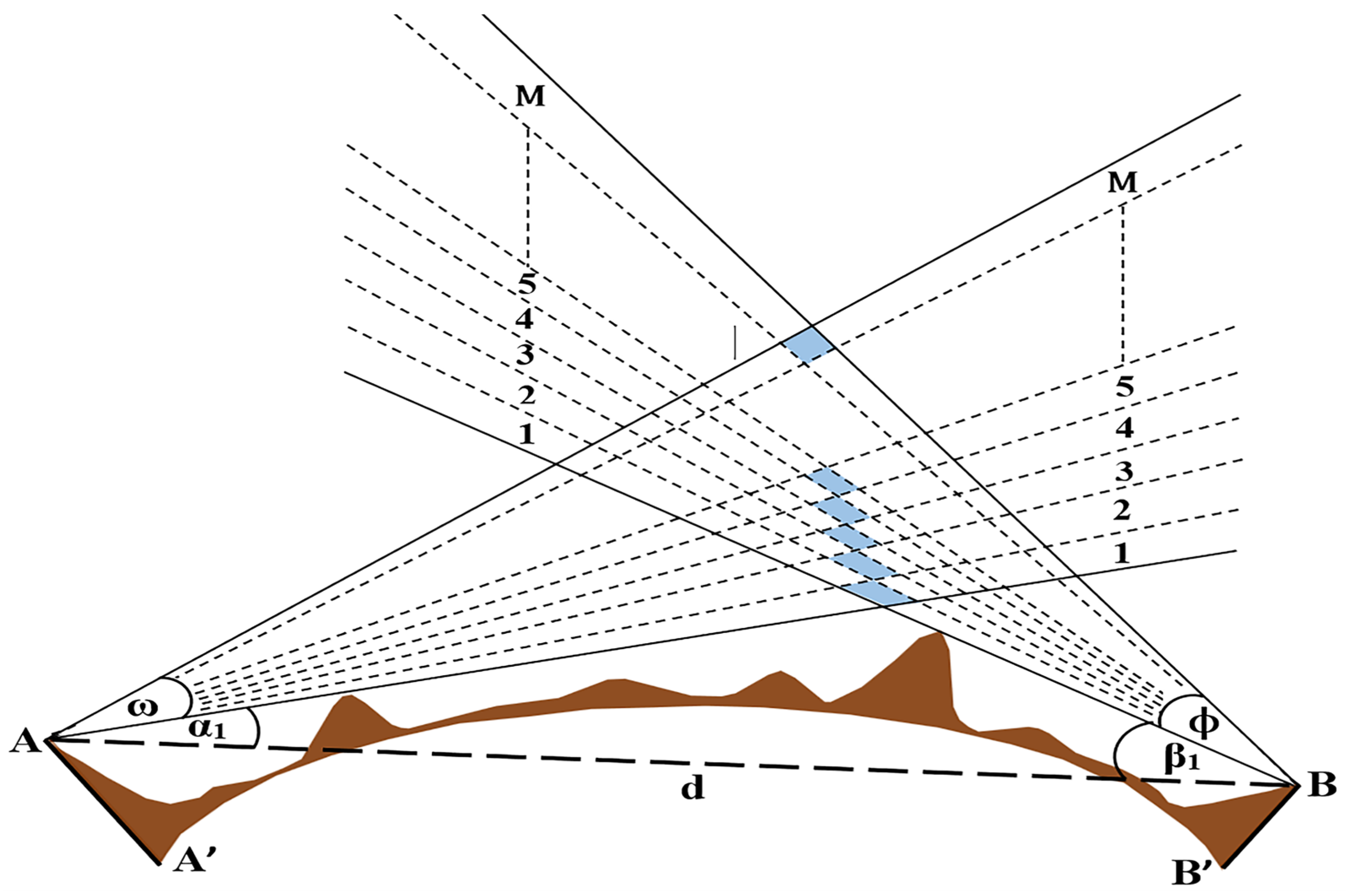
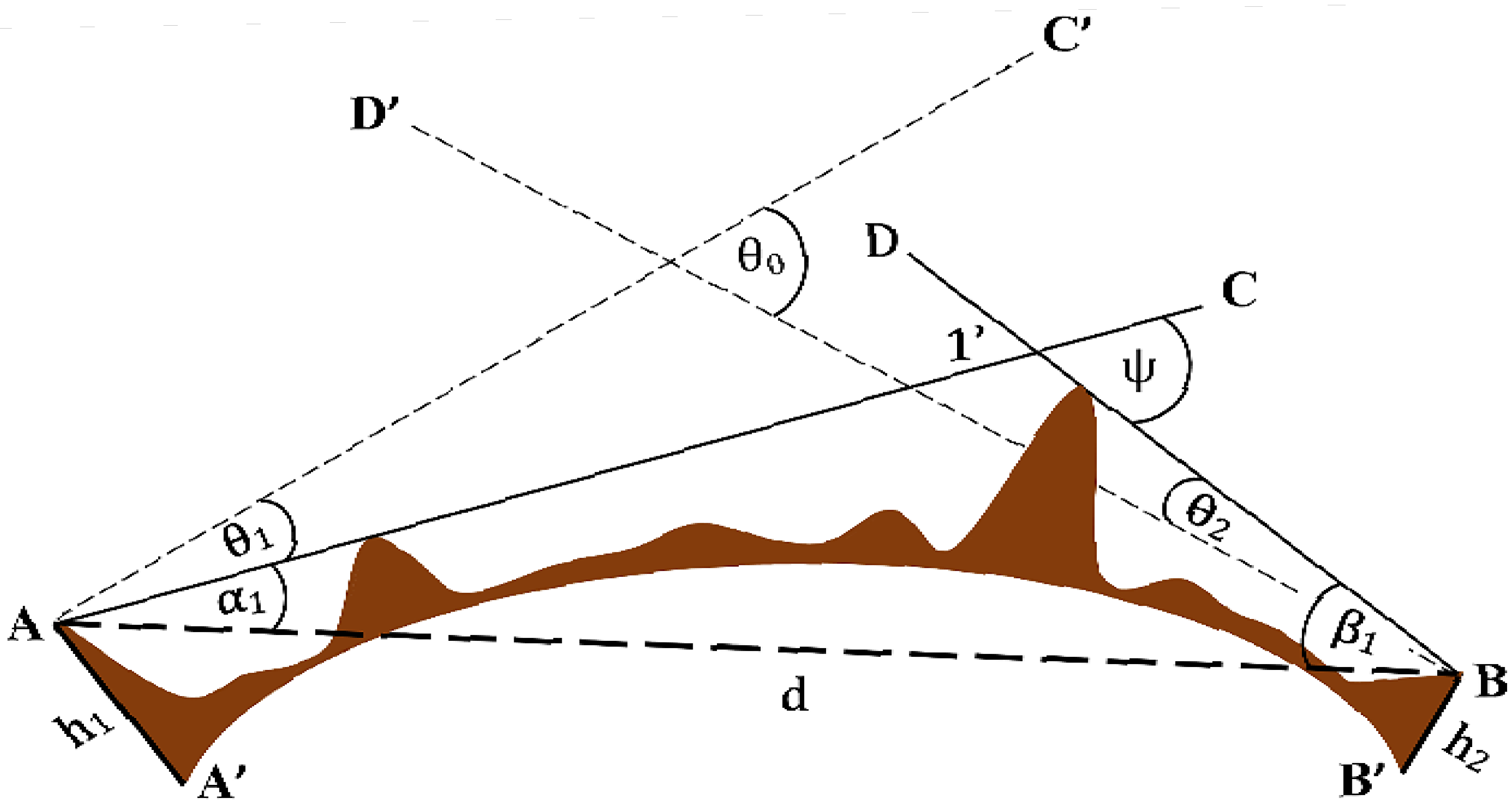
2. Methodology for Determination of Beam Pointing Dynamics

Consider a tropo link between stations A and B, as shown in Figure 1. A is considered a transmitter, and B is considered a receiver for the purpose of explanation. Both the transmitter and receiver are capable of steering their antenna beams to N different elevation angles. The lowest transmit and receive antenna beams just clear their respective horizons, with elevation angles of α 1 and β 1 radians, with respect to straight-line AB. As the transmit and receive beams are steered upward simultaneously, through N different elevation angles, they form common volumes of 1, 2, 3, and so on, till common volume N. Successive common volumes may be contiguous or partially overlapping, depending on the difference between the successive elevation angles. A case of contiguous and vertically stacked common volumes is shown in Figure 1. The heights of the uppermost and lowermost points of a common volume from the Earth’s surface determine its vertical height range. For example, points 1′ and 1′′ in Figure 1 represent the lowermost and uppermost points of the first common volume, and the difference between their heights determines the vertical range of the first common volume. The power received for a given set of corresponding transmit and receive beam elevation angles depends on the propagation conditions in the height range occupied by the corresponding common volume. The received power is calculated using a channel model at different times of the day in different seasons for each of the N sets. A comparison of N-received power values obtained for a given time helps determine the elevation angle set for which the received power is maximum at that time. The height range of the corresponding common volume is most favorable for signal propagation at that particular time. Antenna beams, at any point in time, should be steered such that they have elevation angles offering the maximum received power and their common volume occupies the most favorable height range. Received power for elevation angle sets higher than a certain value and their respective common volume height ranges will be comparatively low at all times. The useful steering range should be restricted to elevation angles below these low-power delivery angles.

2.1. Derivation of Expression for Received Power

The size of the common volume and its height range, in a long-distance tropo link, are considerably large in spite of the narrow beamwidth (1° to 2°). Propagation conditions depend on the scattering properties of the troposphere, which change with height even within the same common volume, owing to its large size. In order to factor in the effect of changing scattering conditions within a given common volume, transmit and receive antenna beams are considered to comprise M sub-beams each. Each set of corresponding transmit and receive sub-beams encloses a portion of the common volume called the sub volume. The value of M is chosen in such a way that the height range of each sub volume is small enough to assume uniform scattering conditions within the sub volume.
Figure 2 shows the splitting of the lowest transmit and receive antenna beams into M sub-beams. Sub volumes, formed by the intersection of the corresponding transmit and receive sub-beams, are always contiguous and vertically stacked, shown as shaded regions in Figure 2. The received power is separately calculated for each of the M sub-beam sets, thus taking into consideration the scattering conditions at different heights. The total received power for a given set of corresponding transmit and receive antenna beam elevation angles is obtained by adding the received powers for its M sub-beam sets. The received power for each of the N sets is calculated using this method.

2.2. Dinc’s Ray-Based Model

Power transmitted in any transmit sub-beam is scattered by the scatterers present in the corresponding sub volume and is received at the receive antenna in the corresponding received sub-beam. The expression of the power received, for any sub-beam set, is given by Dinc et al. [19], using the bistatic radar range equation as follows:
P r ( i , j )   =   P t   G t   G r   σ V ( i , j )   d V c ( i , j )   λ 2   ρ ( 4 π ) 3 R t ( i , j ) 2 R r ( i , j ) 2       watts
Subscript ( i , j ) denotes jth transmit and receives the sub-beam set for the ith elevation angle of antenna beams or the jth sub volume of the common volume formed by the antenna beams with ith elevation angle. For example, in Figure 2, j varies from 1 to M while i remains 1 since the lowest set of transmit and receive antenna beams is shown in the figure. However, i can take any value from 1 to N, as shown in Figure 1. The total power received for the ith set of transmit and receive beam elevation angles is obtained as follows:
P r ( i ) = j = 1 M P r ( i , j )       watts   i ( 1 , N )
P t in Equation (1) is the power transmitted in any transmit sub-beam in watts while G t and G r are the gains of transmit and receive antennas, respectively. P t , G t , and G r are considered equal for all sub-beams. λ is the wavelength in meters, corresponding to the transmit carrier frequency. ρ is the factor that accounts for the polarization mismatch between transmit and receive sub-beams with a value lying between 0 and 1. The value of ρ has been taken as 1 in this paper for all sub-beams, assuming no loss due to polarization mismatch. R t ( i , j ) and R r ( i , j ) are the distances of the sub volume center from transmit and receive antennas, respectively.
σ V ( i , j ) is the differential scattering cross section of the sub volume per unit volume of turbulence in the sub volume. d V c ( i , j ) is the size of the sub volume. The final expression for P r ( i , j ) has been given in [19] as follows:
P r ( i , j )   = P t   G t   G r   π 2 ( ψ ( i , j ) 2 )     ( δ n δ z ) ( i , j ) 2 21.64   λ 2   R t ( i , j ) 2 + R r ( i , j ) 2     s i n ( ψ ( i , j ) ) ·   L 0 ( z ) 4 3 ( ψ ( i , j ) 2 ) 11 3   watts
where d ω is the vertical beamwidth of any transmit or receive sub-beam in radians. ψ ( i , j ) , known as the scatter angle (Appendix A), is the angle in the radians made by the direction of the incident EM ray with a scattered ray. It has been taken as the angle between the lowest rays of the ( i , j ) th transmit and receive sub-beams in this paper. ( δ n δ z ) ( i , j ) is the vertical gradient (Appendix B) of the refractive index n with a height z above the Earth’s surface in the ( i , j ) th sub volume. L 0 ( z ) is the outer scale of turbulence, in meters, and k is the wavenumber given as 2π/ λ .

2.3. Modified Model

The expression for the received power given in Dinc’s ray-based model requires certain modifications for a more realistic and accurate representation of the tropospheric conditions. The expression for σ V ( i , j ) used by Dinc is the acoustic cross section per unit volume of a random medium given in [21] and is applicable for the propagation of sound waves. However, tropospheric communication involves the propagation of EM waves in a turbulent tropospheric medium. Hence, this paper uses a scattering cross section per unit volume of a random medium applicable for EM waves, given in [21] as follows:
σ V ( i , j ) = 2 π k 4   s i n 2 ( X )   φ ( i , j )         m 1
where φ ( i , j ) is the spectral density of refractive index fluctuations in the sub volume. k is the wavenumber given as 2 π λ , and λ is the transmission wavelength. X is the angle between the direction of the incident electric field in the sub volume and the direction from the sub volume to the receiver. Since power is received only due to forward scattering toward the receiver, X is always equal to π 2 and, hence, s i n 2 ( X )   is equal to 1 for any sub volume.
Expression for φ ( i , j ) , based on the Kolmogorov spectrum is given from [21] as follows:
φ ( i , j ) = 0.033   C n ( i , j ) 2 ( κ ( i , j ) ) 11 3           m 3
where κ ( i , j ) is the turbulence wave number in the sub volume. It is given as κ ( i , j ) = 2 π /l, where l represents the size of turbulent eddies or scatterers in meters. C n ( i , j )   2 is the refractive index constant structure representing the strength of atmospheric turbulence in the sub volume, given from [22] as follows:
C n ( i , j ) 2 = 2.8   ( δ n δ z ) ( i , j ) 2 L 0 ( z ) 4 3
The Kolmogorov spectrum is most suitable for modeling φ ( i , j ) , as it is a realistic spectrum, accurately representing the physical characteristics of tropospheric turbulence. As per the Kolmogorov theory, atmospheric turbulence has an outer scale L 0 and an inner scale l 0 . Based on atmospheric studies [23], the value of L0 lies between 10 and 100 m and l0 between 1 and 10 mm. Turbulence characteristics can be divided into three regions according to the size of scatterers relative to these scales viz.: input range, inertial range, and dissipation range [23]. Large-sized eddies (scatterers) are formed in the input range due to the thermal and kinetic energy of the atmosphere. They break down successively into smaller-sized eddies in an inertial range with very little loss of energy. Finally, in the dissipation range, the kinetic energy of the eddies is dissipated through viscous friction when the eddy size becomes very small. The size of the scatterers in inertial range lies between l 0 and L 0 , which is ideal for microwave scattering. Correspondingly, κ ( i , j ) lies between 2 π L 0 and 2 π l 0 .
The ray-based model given by Dinc assumes the troposphere to be a stationary random medium with the size of scatterers in a given sub volume remaining constant over time. Hence, φ ( i , j ) has been calculated in Dinc’s model for a fixed value of κ ( i , j )   in a given sub volume. κ ( i , j )   in the ( i , j ) th sub volume is given as 2 k   s i n   s i n   ( ψ ( i , j ) 2 ) , where k is constant for a given tropospheric system and ψ ( i , j ) is constant for a given sub volume. However, turbulence in the troposphere is not stationary, as large-sized eddies successively break down into smaller-sized eddies at all times. Hence, the size of scatterers is not constant but varies with time, lying between the inner and outer scales of turbulence. Hence, in this paper, the turbulence wave number κ ( i , j )   has been considered a uniformly distributed random variable lying between limits 2 π L 0 and 2 π l 0 , in contrast to Dinc’s model, which uses a fixed value of κ ( i , j ) for a given sub volume.
The expression for differential common volumes used in this paper differs from the simplified expression used in Dinc’s work. The expression for d V c ( i , j ) , as given in [24], is as follows:
d V c ( i , j ) = 1.206   R t ( i , j ) 2   R r ( i , j ) 2   (   ω M )   ( ϕ M   )   ω   ϕ R t ( i , j ) 2   ( ω ) 2 + R r ( i , j ) 2   ( ϕ ) 2   1   s i n ( ψ ( i , j ) )         m 3
ω and ω are the elevation and azimuth beamwidths of transmit antenna, while ϕ and ϕ are the elevation and azimuth beamwidths of receive antenna, respectively. The elevation beamwidths of transmit and receive sub-beams are ω M and ϕ M due to the vertical division of the antenna beams into M sub-beams. However, the azimuth beamwidths of transmit and receive sub-beams remain the same as those of the respective antenna beams, as no division of the antenna beams in the azimuth direction is considered. Parabolic dish antennas for transmitter and receiver, with equal azimuth and elevation beamwidths, i.e., ω = ω and ϕ = ϕ , have been considered in this paper. Moreover, transmit and receive antennas have been considered as having equal dimensions with beamwidths ω and ϕ as equal. Hence, Equation (7) can be written as follows:
d V c ( i , j ) =   1.206     R t ( i , j ) 2   R r ( i , j ) 2   ω   ( ω M ) 2   R t ( i , j ) 2 + R r ( i , j ) 2         s i n ( ψ ( i , j ) )         m 3
Implementing these modified expressions of σ V ( i , j ) , φ ( i , j ) , and d V c ( i , j ) from Equations (4), (5) and (8) in Equation (1), the expression for received power as per the modified ray-based model is given as follows:
P r ( i , j )   = P t   G t   G r     ω   ( ω M ) 2   ( δ n δ z ) ( i , j ) 2   1.82 λ 2 R t ( i , j ) 2 + R r ( i , j ) 2   s i n   ( ψ ( i , j ) )     ·   L 0 ( z ) 4 3 ( κ ( i , j ) ) 11 3   watts

3. Data Collection and Processing

Link geometry details and system parameters for the two different tropospheric links discussed in this paper have been worked out by synthesizing the links using the Tropo Link Implementation and Planning Software (TLIPS). The transmitter location for the first link is near Vijapur, Gujarat (India), and the receiver location is near Sahij, Gujarat (India), with the common volume of the link formed over Ahmedabad, Gujarat (India). The transmitter location for the second link is near Bhukuradia, Assam (India), and the receiver location is near Bherakuchi, Assam (India), with the common volume of the link formed over Guwahati, Assam (India). The links belong to different climate types. Ahmedabad experiences a hot and semi-arid climate, while Guwahati has a warm and temperate climate. Thus, the results and conclusions obtained in this paper are based on a broad study of tropospheric links belonging to different climate types.
The parameters obtained from the Ahmedabad and Guwahati links are given in Table 1. In the case of the Ahmedabad link, the number of sub-beam sets (M) has been taken as 10 for this paper, as it gives a vertical height range of each sub volumes close to 150 m. In the case of the Guwahati link, the number of sub-beam sets (M) has been taken as five due to the narrow beam width of transmit and receive antennas, which gives a vertical height range of each sub volumes close to 180 m. The selection of M for both links has been chosen keeping in mind the fact that the atmospheric conditions within a vertical distance of 200 m remain almost the same, as observed from the meteorological data obtained from the Indian Meteorological Department (IMD).
The calculation of the refractive index gradient requires meteorological parameters of atmospheric pressure, temperature, and dew point temperature. These parameters have been obtained from the Ahmedabad and Guwahati observatories of IMD. Meteorological observatories of IMD make radio sonde measurements of these parameters for heights ranging from the Earth’s surface up to 20 Kms, two times in a day, at 05:30 a.m. and 05:30 p.m. However, observatories are not able to record data on all days of the year due to maintenance and other activities. The meteorological data for both observatories were obtained from 2005 to 2021. It was found that the Ahmedabad observatory had the maximum number of recordings for the year 2006, while the Guwahati observatory had the maximum number of recordings in the year 2019. Hence, the meteorological data from the year 2006 were used in the case of the Ahmedabad link, and the year 2019 was used in the case of the Guwahati link for the determination of beam pointing dynamics for these links.
The calculation of the received power using the modified model, given in Equation (9), requires the determination of various system and link geometry parameters along with a refractive index gradient. Certain system and link geometry parameters, like transmit power ( P t ), transmit and receive antenna gains ( G t , G r ), antenna beam widths ( ω , ϕ ), and transmission wavelength (λ), are outlined in Table 1. However, other parameters, like the scatter angle ( ψ ( i , j ) ), the distances of sub volume center from transmit and receive antennas ( R t ( i , j ) , R r ( i , j ) ), the vertical gradient of refractive index ( δ n / δ z ), the outer scale of turbulence ( L 0 ( z ) ), and the turbulence wave number ( κ ( i , j ) ) need to be calculated. The calculations of these parameters are shown in Appendix A, Appendix B and Appendix C.

4. Results and Discussions

Received powers have been calculated for 11 different sets of transmit and receive beam elevation angles for both links, taking N as 11. The common volumes formed by antenna beams with successive elevation angles are overlapping for both links. The transmit and receive beam elevation angles for different sets and height ranges of corresponding common volumes are given in Table 2. The difference in elevation between the lowest and highest beams is 1.75 degrees for the Ahmedabad link and 2.1 degrees for the Guwahati link, while the difference in height between the lowest and highest common volumes is 3082.7 m for the Ahmedabad link and 2719.7 m for the Guwahati link. Hence, the propagation characteristics of the tropospheric region over approximately 3 kms vertical extent were examined to determine the beam pointing dynamics of both links. The received power was calculated for each of the 11 sets of the beam elevation angles, for morning as well as evening times (0530 and 1730 IST), using IMD data from the Ahmedabad observatory for the year 2006 and from the Guwahati observatory for the year 2019. The maximum power, amongst the powers received for different elevation angles, has been determined for both times on each of these days.

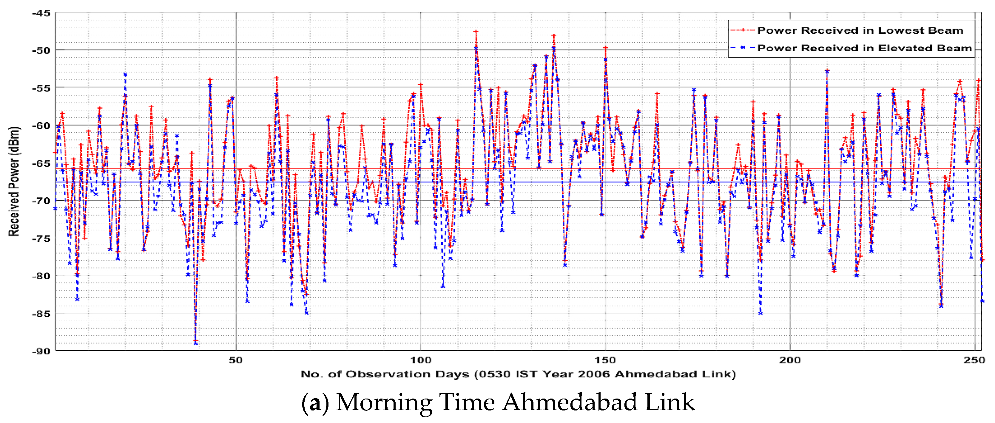
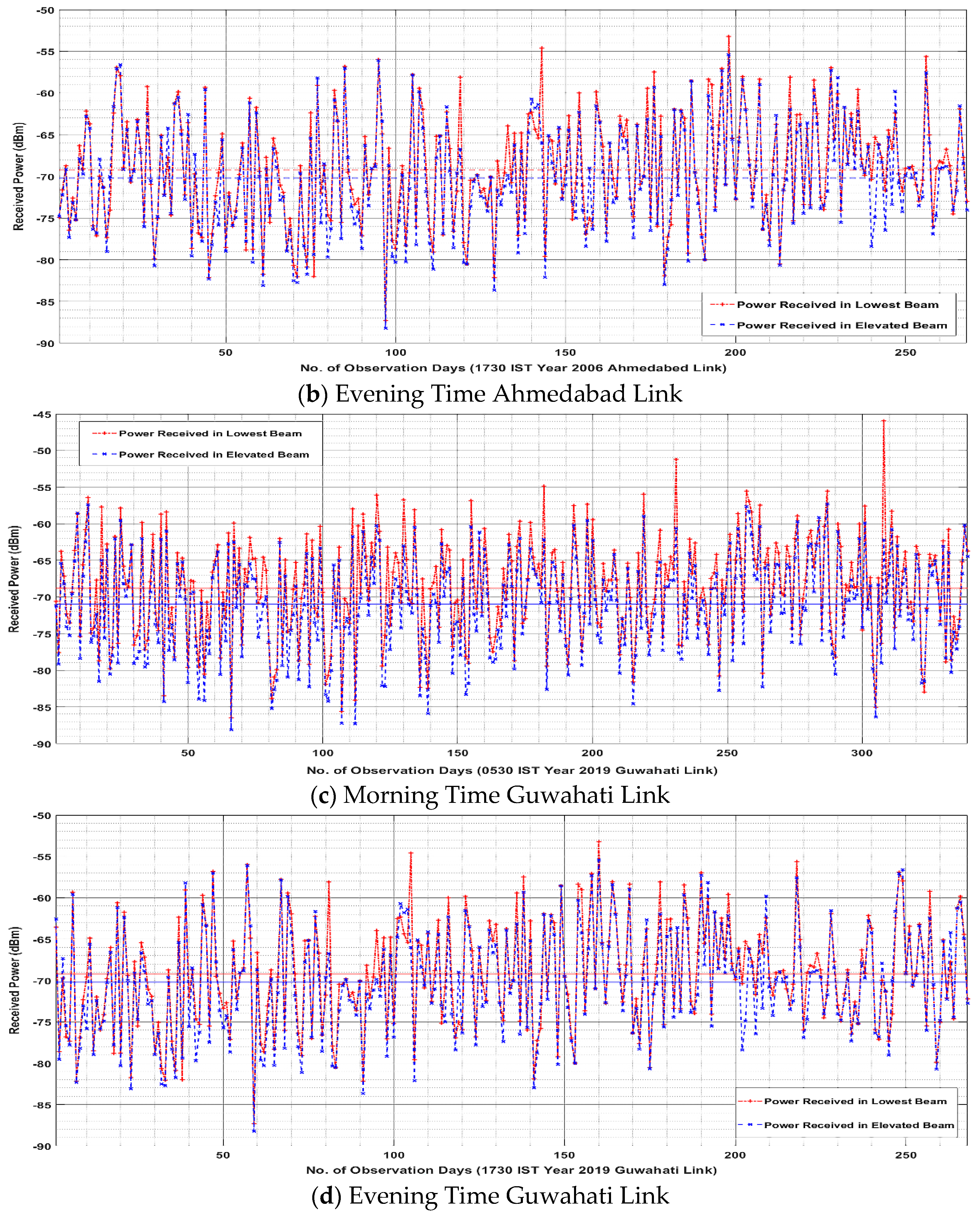
4.1. Results for Ahmedabad Link

Figure 3 shows the day-to-day comparison between the maximum power received (out of the received powers for all 11 sets) and the received power for the lowest (first) set of transmit and receive beam elevation angles, for morning and evening times, in summer and winter seasons, for the Ahmedabad link. It was found that the maximum power was received from beam sets other than the lowest beam set (elevation angle 1) at multiple instances. For morning times, the maximum power was received from elevated beams (elevation angles 2 to 11) for 15% of the days in the year, mostly from beam sets 2 to 5. The maximum power received was greater than the power received for the lowest elevation beam set by more than 1 dB on 5% of the days and was even more than 3 dB on a few occasions. The largest difference between the maximum power and the lowest elevation beam power in the morning time, when considered for all of the available days, was found to be 4.12 dB in the month of May. For the evening time, the occasions when the maximum power was received from elevated beams increased to 21% of the days in the year. Days when the difference between maximum power and lowest elevation beam power was more than 1 dB, increased to 8% in evening time and the instances of a more than 3 dB difference doubled. The maximum difference between the maximum power and the lowest elevation was found to be 6.05 dB in the month of June. Comparing the results obtained for the summer and winter seasons, the average received power was higher in the summer seasons. The maximum power in the summer was received mostly from elevated beams, especially in the evening. The maximum power was received from almost all beams (elevation angles 1 to 10) on different occasions in the year, except from the beam with an elevation angle of 11.

4.2. Results for Guwahati Link

The maximum power, in morning time 0530 IST, was received from elevated beams (elevation angles 2 to 11) for 5% of the days in the year, mostly from beam sets 2 to 4. For the evening time 1730 IST, the occasions when the maximum power was received from elevated beams increased to 16.5% of days in the year. As in the case of the Ahmedabad link and the Guwahati link as well, the maximum power during the evening time was received from almost all of the elevated beams (elevation angles 2 to 10) on different occasions, except from the beam with an elevation angle of 11. The maximum difference between the maximum power received and the lowest elevation angle beam set received power, when considered for all of the available days, was found to be 1.54 dB in the month of May for the morning time and 4.19 dB in the month of March for the evening time. Comparing the results obtained for the summer and winter seasons, the average received power was higher in the summer seasons, but the difference was not as prominent as for the Ahmedabad link. The maximum powers in the summer were again received mostly from elevated beams, especially in the evening.

4.3. Discussions

The maximum transmit power ( P t ), gains of transmit and receive antennas ( G t   ,   G r ), and antenna beam widths ( ω , ϕ ) are the system design parameters that are mostly fixed for a given tropospheric link. The outer scale of turbulence ( L 0 ) and turbulence wave number ( κ ) are considered random numbers due to the time-varying nature of atmospheric turbulence. The calculation of received power for any beam elevation angle involves multiple iterations with a randomly selected value of L 0 and κ for each iteration and averaging over all of the iterations. Therefore, the effects of L 0 and κ on the received power are the same for any beam elevation angle. The parameters in the expression for received power given in Equation (9) that actually affect the powers received for different sets of transmit and receive beam elevation angles are the vertical gradient of refractive index ( δ n / δ z ), sub volume distances ( R t ,   R r ), and scatter angle ( ψ ). R t , R r , and ψ have the effect of decreasing the received power with an increase in the elevation angle. Hence, for the received power in any elevated beam to be higher than the lowest elevation beam, δ n / δ z in the common volume enclosed by the elevated beam should be large enough to deliver a higher power in spite of increased losses due to elevation.
Observations made on the Ahmedabad link for morning time of 5 June 2006 are discussed for a clear understanding of the reason behind the elevated beams delivering maximum received power. On 5 June 2006 at 0530 IST, for the Ahmedabad link, the maximum power was received in the beam set 8 and was 3.78 dB more than the power received in the lowest (first) beam set, as shown in the highlighted portion of Figure 4. In order to understand the reason behind this high power in an elevated beam, the variation of ( d n / d z ) 2 with height on 5 June 2006 at 0530 IST is shown in Figure 4. Taking the average values of ψ , R t , and R r for different beam sets, it was seen that these parameters induce an additional loss of 6 dB for beam set 8 when compared to lowest beam set. However, as seen in Figure 4, ( d n / d z ) 2 has a distinct peak at around 1935 m along with other smaller peaks that fall in the height range of the common volume formed by the beam set 8 and are above the common volume height range of the lowest beam set. The average value of ( δ n / δ z ) 2 for beam set 8 was found to be approximately 9.5 times higher than for the lowest beam set, which gives a gain of 9.78 dB in the power received for beam set 8. Hence, as a result, the received power for beam 8 was 3.78 dB higher than the lowest beam.
The main reason for this peak in ( δ n / δ z ) 2 is a sharp inversion in the vertical gradient of the atmospheric refractive index. It was observed that n decreases gradually from Earth’s surface up to a height of 1935 m and then suddenly increases between 1935 m and 1983 m. This inversion in vertical gradient of n is associated with a variation in the atmospheric vapor pressure, which was found to increase from 16.5 mb at 1935 m 20.13 mb at 1980 m. Smaller peaks observed after the main peak in Figure 4 are due to a sharp decrease in the refractive index in height ranges of 2115–2252 m and 2539–2855 m, attributable to a sharp fall in the vapor pressure in both these height ranges. Thereafter, n decreases gradually up to an observed height of 3332 m. Both a sharp increase and a sharp decrease in the vapor pressure result in a peak in ( δ n / δ z ) 2 . However, increase in the vapor pressure cause an inversion in the slope of vapor pressure with height. This inversion produces more pronounced peaks in ( δ n / δ z ) 2 compared to a sharp decrease in the vapor pressure. The inversion of vapor pressure can be due to cloud formation at heights of 2000 m and above. This explains the few occasions when very high levels of power were received from beams with elevation angles of 5 and above, mostly in the monsoon season. Variation in the vapor pressure was investigated, for the Ahmedabad as well as Guwahati links, on all those days when the maximum power was received from an elevated beam set. In all these cases, it was found that there was either a sharp fall or increase in the vapor pressure between certain heights falling in the common volume height range of the elevated beam set.
Temperature during the night is generally low, and due to this, the water vapor content in the air becomes high, which being heavier than air, settles close to Earth’s surface. This results in high vapor pressure at low heights, which decreases rapidly with increases in height. A sharp gradient of vapor pressure is thus observed from ground level only up to lower heights. This explains why maximum powers at 0530 IST were mostly received from beams with lower elevation angles, one to five, on the Ahmedabad link and from beams with elevation angles of one to four on the Guwahati link. However, during the daytime, the Earth’s surface is heated up by the Sun’s rays, which in turn, heats up the atmosphere at lower heights. Direct heating of the atmosphere from the Sun’s rays also takes place. As a result, the water vapor content of air moves upwards, setting up a large gradient of vapor pressure even at higher heights. This explains the reason behind maximum powers being obtained from beams with almost all elevation angles (1 to 10) at 1730 IST on both the links. Heating of the atmosphere is more prominent in the summer season, especially in the evening hours. This results in a considerable upward shift in the vapor content and the development of large gradients of refractive index at all heights. Hence, the average received power is higher in the summer season, with more instances of maximum power being received from beam sets with higher elevation.
The results indicate that for the Ahmedabad link, beam sets 1 to 5, corresponding to the height range of 249.3–2406.0 m, and for the Guwahati link, beam sets 1 to 4, corresponding to the height range of 323.8–1764.2 m, are more favorable for beam steering during the morning hours. Hence, beam steering should be restricted to the elevation angles of these beam sets. However, in the evening hours, beams with higher elevation angles are also favorable. Hence, beam steering should be carried out over the entire range of elevation angles 1 to 10. Beams with very high elevation angles like 11 rarely give high received powers. Hence, steering the beam to an elevation angle of 11 and higher will be a waste of resources and should be avoided. Thus, it can be seen that the beam pointing dynamics of a tropospheric link can be determined using a modified ray-based model with real-world meteorological data, and the knowledge obtained can be used for efficient beam steering.

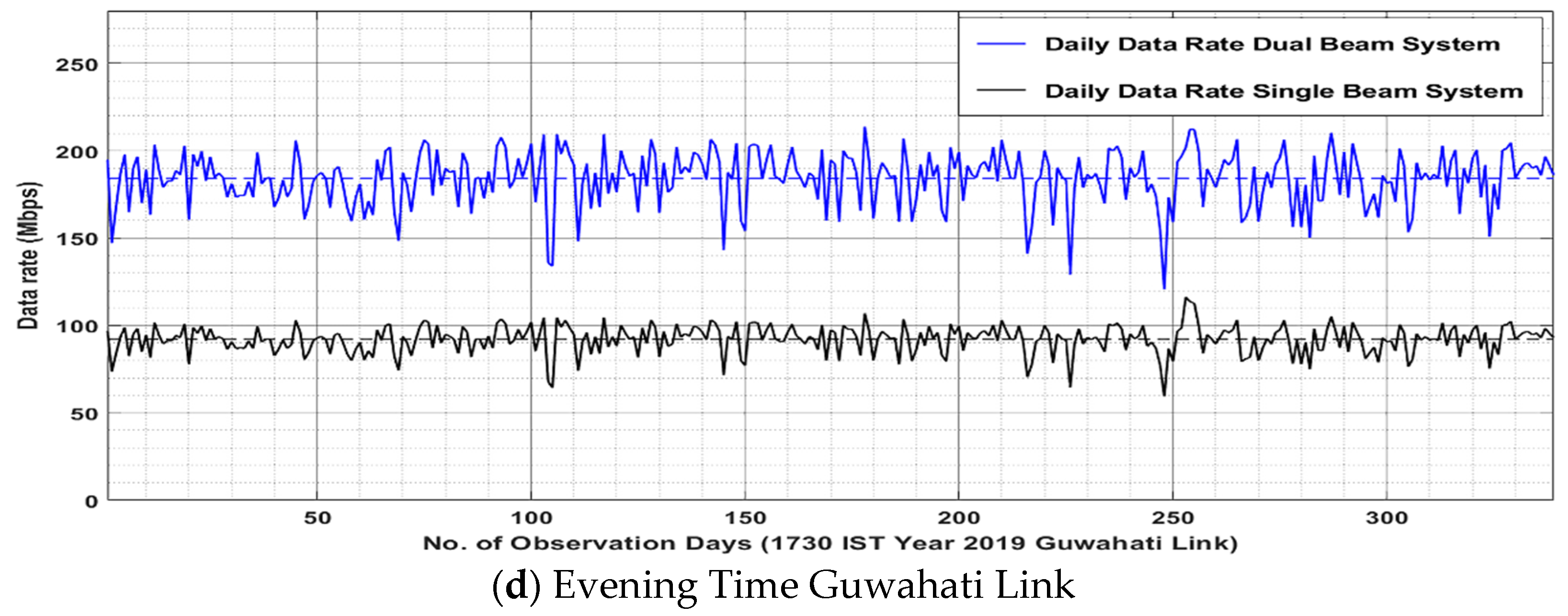
4.4. Dual Data Streaming Design

An important result emerged from the determination of beam pointing dynamics for Ahmedabad and Guwahati links. It was found that for the Ahmedabad link, at the morning time of 0530 IST, for all of the days in the year, the received power in at least one of the elevated beam sets was either higher or lower than 4 db compared to the power received in the lowest beam set. A similar observation was made on 95% of the days for the evening hours of 1730 IST. For the Guwahati link, the same observation was made on 97% of days for the morning time and 99% of the days for the evening hours.
Figure 5 shows the received power, P r ( i ) , obtained for the lowest beam (i = 1) and the elevated beam (i = 2 to 10, whichever delivers the highest power at different times) for both the Ahmedabad and Guwahati links on all the observation days at 0530 IST as well as 1730 IST. The results show that the power received in one of the elevated beams is either higher or lower, but within 4 dB of the power received in the lowest beam at all times. Also, the differences between the yearly averages of the received power in the lowest and elevated beams on both links for morning as well as evening times are within 2 dB. Thus, it can be deduced from the obtained results that at any given time, there are at least two beam sets delivering high powers, with a difference of less than 4 dB between them. Hence, dual data streaming is possible on tropospheric links with dual beams between the transmitter and receiver. Also, as highlighted earlier, the lowest beam set delivers the highest power in almost 80–85% of the time. Thus, one set of transmit and receive beams in a dual-beam design should have fixed elevation angles corresponding to those of the lowest (first) beam set, just to clear their respective radio horizons. The second set of antenna beams should be dynamically steered with variable elevation angles corresponding to the elevation angles of beam set 2s to beam set 10. Elevation angles of steerable antenna beams, at any given time, should depend on whichever beam set (amongst beam sets 2 to 10) is giving the maximum received power at that time.
Figure 6 shows the basic design of a tropospheric communication system for dual data streaming using two beams. Solid rays forming the lowest common volume, shown as the shaded region, depict the fixed-beam set. Elevation angles of fixed transmit and receive beams are α 1 and β 1 , respectively. Dashed rays forming common volumes shown in the pattern fill depict the dynamically steerable beam set with elevation angles variable from ( α 2 , β 2 ) to ( α n , β n ). Conventional tropo systems employ quad diversity with two different and physically separated transmit and receive antennas. Each transmit antenna transmits two different frequencies: one vertically polarized and the other horizontally polarized. Similarly, each receiving antenna receives two different frequencies with orthogonal polarization. Quad diversity, i.e., a combination of space and frequency diversity, is necessary to mitigate the effect of fast fading through diversity combining. The dual-beam design should also incorporate quad diversity with two different beams from each of transmit antenna. Different beams from the same antenna may transmit at the same frequency, with individual data streams coded with orthogonal codes to minimize interference.
Troposcatter systems conventionally use single transmit and receive antenna beams clearing their respective horizons or highest obstructions in front of the transmit and receive antennas, i.e., the transmit and receive antenna beams with the lowest possible elevation angles, represented by solid rays in Figure 6. The performance of a conventional design using a single beam and a dual data streaming design using two beams needs to be compared in terms of achievable data rates. In order to make the comparison, the received Signal-to-Noise Ratio (SNR) has been calculated for fixed beams and dynamic beams separately, using values of the received power from Equation (9) for all the available days of the year as follows:
S N R f i x = 30 + 10 { j = 1 M P r ( 1 , j )   }   L a N 0 dB i 2   t o   N S N R d y n = 30 + 10 [ { j = 1 M P r ( i , j )   }   ]   L a N 0 dB
where N 0 is the average noise power. N 0 has been obtained as −101 dBm, using a noise floor of −174 dBm per Hz and a bandwidth of 20 MHz for the Ahmedabad link. For the Guwahati link, N 0 has been obtained as −104 dBm, using a noise floor of −174 dBm per Hz and a bandwidth of 10 MHz, as highlighted in Table 1. In a practical system, additional fixed losses ( L a ) , like noise figure, waveguide loss, connector loss, circulator loss, and coupling loss (measurement loss), will reduce the SNR of both the fixed beam and dynamic beam. L a has been taken as approximately 10 dB for both links. Though the tropospheric channel is a Rayleigh fading channel, space and frequency diversity combining in tropo systems removes the effect of fast fading and renders the channel an AWGN channel. Hence, achievable data rates have been calculated for both beams using Shannon’s channel capacity theorem for AWGN channels as follows:
D a t a   R a t e f i x = B     ( 1 + S N R f i x )       D a t a   R a t e d y n = B     ( 1 + S N R d y n )  
where B is the channel bandwidth given as 20 MHz. Theoretically, an achievable data rate for a conventional single-beam system will be equal to the data rate of a fixed beam obtained from Equation (11), while for a dual data streaming system with two beams, the data rate will be equal to the sum of the data rates of a fixed beam and a dynamic beam obtained from Equation (11).
Figure 7 shows a comparison of the theoretically achievable data rates using a conventional fixed single-beam system and dual data streaming two-beam systems on both the Ahmedabad and Guwahati links at 0530 IST and 1730 IST. Dashed lines in blue and black depict the average daily data rate for a year. It can be clearly seen that the average daily data rate for dual data stream designs is almost double that for a single-beam design, in all cases.

5. Conclusions

Steering antenna beams in tropospheric communication systems to heights delivering high received power overcomes slow fading, improves link availability, and enhances the achievable data rates. Beam pointing dynamics provides knowledge about favorable angles or heights for beam steering at different times of the day and in different seasons. It also helps determine the height limit up to which steering would be useful. This knowledge will help develop an efficient, faster, and more focused beam steering approach. The important contributions made in this paper are the development of a modified ray-based model that gives a more realistic representation of tropospheric propagation characteristics than Dinc’s ray-based model. A detailed methodology for the determination of the beam pointing dynamics of a link is also presented using the modified model. Beam pointing dynamics for two links with different climate types, located in the Indian states of Gujarat and Assam, have been obtained using the given methodology with real-world data on atmospheric parameters obtained from IMD. The results given in the paper show received power levels obtained for different beam positions on both links, establishing the fact that beam steering can help achieve higher data rates. This paper also explains the reason for the higher received power obtained from elevated beams by discussing refractive index gradients on the Ahmedabad link on a specific day. The current work on tropo systems suggests that antenna beams with the lowest elevation angles always deliver the highest power, as any increase in the elevation angle of the beams introduces losses. This makes the discussion novel and path-breaking as it proves that elevated beams can deliver higher powers and, hence, builds a case for beam steering in tropo systems. Another significant contribution of the paper is the fact that it presents the prospect of dual data streaming on tropo links using a dual-beam design with a fixed beam with the lowest elevation angle and a dynamically steered elevated beam. This prospect is supported by the results showing that there is at least one elevated beam delivering power that is either higher or close to the power delivered by the lowest beam. The results show a comparison of the theoretically achievable data rates for single-beam and dual-beam systems. The results show that dual data streaming using a dual beam can significantly enhance the data-carrying capacity of tropospheric links as compared to conventional single fixed-beam designs.

Author Contributions

Conceptualization, A.G. and R.M.; methodology, A.G. and A.K.K.; validation, A.G. and A.K.; formal analysis, R.M. and A.K.; resources, A.G. and A.K.K.; data curation, A.G.; writing—original draft preparation, A.G. and R.M.; writing—review and editing, A.G. and A.K.; visualization, A.G. and A.K.K.; supervision, R.M. and A.K.K.; project administration, A.K. All authors have read and agreed to the published version of the manuscript.

Funding

This research received no external funding.

Data Availability Statement

The original contributions related to tropospheric link parameters, presented in the study, are included in the article, further inquiries can be directed to the corresponding author/s. Restrictions apply to the availability of meteorological data. Data were obtained from Indian Meteorological Department (IMD) and are available at https://dsp.imdpune.gov.in with the permission of IMD.

Conflicts of Interest

The authors declare no conflict of interest.

Appendix A. Calculation of Scatter Angle and Sub Volume Distances

The elevation angles of the lowest transmit and receive beams with respect to straight line AB between transmitter and receiver are α 1 and β 1 , respectively, as shown in Figure A1.
α 1 and β 1 are given from [7] as follows:
α 1 = θ 1 + d 2 a + h 1 h 2 d β 1 = θ 2 + d 2 a h 1 h 2 d
AC and BD represent the lower edges of the first transmit and first receive antenna beam, respectively, intersecting in the point 1′. AC’ and BD’ are the horizontals at A and B, respectively. θ 1 and θ 2 are the elevation angles of the respective horizons from the transmitter and receiver with respect to the horizontals AC’ and BD’, respectively. θ 1 and θ 2 may be positive or negative, depending on whether the highest obstacles (horizons) in front of the transmitter and receiver are above or below the horizontals. d is the straight line distance between the transmitter and receiver and, a is the effective Earth’s radius in meters. h 1 and h 2 are the heights of the transmitter and receiver above the Earth’s surface in meters.
Figure A1. Link geometry for calculation of elevation angles.
Telecom 05 00009 g0a1
The elevation angles of ith transmit and receive beams with respect to straight line AB are given as follows:
α i = α 1 + ( i 1 )     Δ α       rad β i = β 1 + ( i 1 )     Δ β       rad
where Δ α is the difference between the elevation angles of successive transmit antenna beams, and Δ β is the difference between the elevation angles of successive receive antenna beams. Both Δ α and Δ β have been taken as equal to 3.1 mrad for the Ahmedabad link and 3.7 mrad for the Guwahati link, considering successive common volumes to be overlapping. α ( i , j ) and β ( i , j ) , elevation angles of the lowest rays of ( i , j ) th transmit and receive sub-beams are given as follows:
α ( i , j ) = α i + ( j 1 ) ω M       rad
β ( i , j ) = β i + ( j 1 ) ϕ M       rad
Scatter angle ψ ( i , j ) for ( i , j ) th sub-beam set can be given from [7] as follows:
ψ ( i , j ) = α ( i , j ) + β ( i , j )       rad
Distances of lowest point of ( i , j ) th sub volume from transmitter and receiver are given from [7] as follows:
R t ( i , j ) = d s i n s i n     β ( i , j )     s i n   ψ ( i , j )       m R r ( i , j ) = d s i n s i n     α ( i , j )     s i n   ψ ( i , j )       m
Distances of highest point of ( i , j ) th sub volume from transmitter and receiver will be R t ( i , j + 1 ) and R r ( i , j + 1 ) .

Appendix B. Calculation of Vertical Gradient of Refractive Index

Vertical height range of ( i , j ) th sub volume lies between its uppermost point h U ( i , j ) and lowermost point h L ( i , j ) , given from [7] as follows:
h L ( i , j ) = h 1 + 1 2 a R t ( i , j ) 2 + { θ 1 + ( i 1 ) Δ α + ( j 1 ) ( ω M ) }   ·   R t ( i , j )       m h U ( i , j ) = h 1 + 1 2 a R t ( i , j + 1 ) 2 + { θ 1 + ( i 1 ) Δ α + j ( ω M ) }   ·   R t ( i , j + 1 )       m
Value of refractivity N at a given point in troposphere can be calculated from ITU-R Recommendation P.452-15 [25], as follows:
N = 77.6 T ( P + 4810   e T )       N-units
where P is the atmospheric pressure in millibars, T is the atmospheric temperature in degree Kelvin, and e is the atmospheric vapor pressure in millibars, measured at the given point. Atmospheric vapor pressure can be obtained from [26] as follows:
e = ( T d + d ) a 10 ^ ( c + [ b T d + d ] )       mbar
T d is the dew point temperature in degree kelvin measured at the given point. Values of constants a ′, b′, c′, and d′ are given in Table A1 [26]. Values of P , T , and T d have been obtained for different tropospheric heights from IMD observatories of Ahmedabad and Guwahati. The value of N has been calculated using these values for different heights lying in the height range of the given sub volume. δ N δ z is then calculated for successive heights and averaged to obtain a single value, ( δ N δ z ) ( i , j ) for the given sub volume. Average values of δ n / δ z for the ( i , j ) th sub volume have been calculated from [27] as follows:
( δ n δ z ) ( i , j ) = ( δ N δ z ) ( i , j ) × 10 6
Table A1. Values of constants for calculation of vapor pressure from dew point.
ConstantValue
( T d > 0 °C)
Value
( T d ≤ 0 °C)
a−4.9283−0.32286
b−2937.4−2705.21
c23.551811.4816
d273273

Appendix C. Selection of Turbulence Wave Number

As already discussed, κ ( i , j ) varies with time and is a random number lying between 2 π L 0 and 2 π l 0 . Hence, the received power P r ( i , j ) has been calculated using the Monte Carlo simulation with a sufficient number of iterations for each calculation. L 0 and l 0 have been considered as uniformly distributed random variables with limits (10 m and 100 m) and (1 mm and 10 mm), respectively. The values of both L 0 and l 0 were selected randomly for each iteration from their respective ranges. κ ( i , j ) for an iteration, has been selected randomly from a uniform distribution with limits 2 π L 0 and 2 π l 0 , corresponding to values of l 0 and   L 0 selected for that iteration. The received power for any sub-beam set, P r ( i , j ) , is obtained by averaging the received power values obtained over all iterations. Finally, the received power for a given set of beam elevation angles is calculated using Equation (2).

References

  1. Marconi, G. Radio communications by means of very short electric waves. IRE Trans. Antennas Propag. 1957, 5, 90–99. [Google Scholar] [CrossRef]
  2. Clavier, A.; Altovsky, V. Beyond-the-horizon 300-magacycle propagation tests in 1941. Elec. Commun. 1956, 33, 117–132. [Google Scholar]
  3. Katzin, M.; Bauchman, R.; Binnian, W. 3- and 9-centimeter propagation in low ocean ducts. Proc. IRE 1947, 35, 891–905. [Google Scholar] [CrossRef]
  4. Day, J.; Trolese, L. Propagation of short radio waves over desert terrain. Proc. IRE 1950, 38, 65–175. [Google Scholar] [CrossRef]
  5. Pekeris, C. Wave theoretical interpretation of propagation of 10- centimeter and 3-centimeter waves in low-level ocean ducts. Proc. IRE 1947, 35, 453–462. [Google Scholar] [CrossRef]
  6. Gunther, F.A. Tropospheric scatter communications past, present, and future. IEEE Spectr. 1966, 3, 79–100. [Google Scholar] [CrossRef]
  7. Roda, G. Troposcatter Radio Links, 1st ed.; Artech House Publishers: Norwood, MA, USA, 1988. [Google Scholar]
  8. Propagation Prediction Techniques and Data Required for the Design of Trans-Horizon Radio-Relay Systems. ITU-R Recommendation P.617-5(08/2019). Available online: https://www.itu.int/rec/R-REC-P.617-5-201908-I/en (accessed on 5 September 2023).
  9. Zhao, Q.; Zhang, R.; Lin, L.; Li, Q. The study of experiment on tropospheric scatter propagation at c-band. In Proceedings of the 12th International Symposium on Antennas, Propagation and EM Theory (ISAPE), Hangzhou, China, 3–6 December 2018; Volume 3. [Google Scholar] [CrossRef]
  10. Soi, S.; Singh, S.K.; Singh, R.; Kumar, A. Link analysis of ku band troposcatter communication. In Proceedings of the 2019 IEEE Mtt-s International Microwave and RF Conference (IMARC), Mumbai, India, 13–15 December 2019; pp. 1–5. [Google Scholar]
  11. Winters, J.H.; Luddy, M.J. Phased array applications to improve troposcatter communications. In Proceedings of the 2019 IEEE International Symposium on Phased Array System & Technology (PAST), Waltham, MA, USA, 15–18 October 2019; pp. 1–4. [Google Scholar] [CrossRef]
  12. Winters, J.H.; Luddy, M.J. Wideband array transmission—Waveforms and phase notching. In Proceedings of the 2019 IEEE International Symposium on Phased Array System & Technology (PAST), Waltham, MA, USA, 15–18 October 2019; pp. 1–4. [Google Scholar] [CrossRef]
  13. Booker, H.G.; Gordon, W.E. A theory of radio scattering in the troposphere. Proc. IRE 1950, 38, 401–412. [Google Scholar] [CrossRef]
  14. Friis, H.T.; Crawford, A.B.; Hogg, D.C. A reflection theory for propagation beyond the horizon. Bell Syst. Tech. J. 1957, 36, 627–644. [Google Scholar] [CrossRef]
  15. Bello, P. A troposcatter channel model. IEEE Trans. Commun. Technolog. 1969, 17, 130–137. [Google Scholar] [CrossRef]
  16. Rice, P.L.; Longley, A.G.; Barsis, A.P.; Norton, K.A. Transmission Loss Predictions for Tropospheric Communication Circuits; Ser. Technical Note no. 101; National Bureau of Standards, U.S. Department of Commerce: Gaithersburg, MD, USA, 1965.
  17. Prediction Procedure for the Evaluation of Interference between Stations on the Surface of the Earth at Frequencies Above about 0.1 GHz. ITU-R Recommendation P.452-17 (09/2021). Available online: https://www.itu.int/rec/R-REC-P.452-17-202109-I/en (accessed on 5 September 2023).
  18. A General Purpose Wide-Range Terrestrial Propagation Model in the Frequency Range 30 mhz to 50 ghz. ITU-R Recommendation P.2001-4 (09/2021). Available online: https://www.itu.int/rec/R-REC-P.2001-4-202109-I/en (accessed on 5 September 2023).
  19. Dinc, E.; Akan, O.B. A ray-based channel modeling approach for mimo troposcatter beyond-line-of-sight (b-los) communications. IEEE Trans. Commun. 2015, 63, 1690–1699. [Google Scholar] [CrossRef]
  20. NAMMA LIDAR Atmospheric Sensing Experiment (LASE). Available online: https://ghrc.nsstc.nasa.gov/uso/ds_docs/namma/namlase/namlase_dataset.html (accessed on 5 September 2023).
  21. Ishimaru, A. Wave Propagation and Scattering in Random Media; Ser. An IEEE OUP Classic Reissue; Wiley-IEEE Press: Hoboken, NJ, USA, 1999. [Google Scholar]
  22. Marzano, F.S.; d’Auria, G. Model-based prediction of amplitude scintillation variance due to clear-air tropospheric turbulence on earth-satellite microwave links. IEEE Trans. Antennas Propag. 1998, 46, 1506–1518. [Google Scholar] [CrossRef]
  23. Devasirvatham, D.M.J. Effects of Atmospheric Turbulence on Microwave and Millimeter Wave Satellite Communications Systems. Ph.D. Dissertation, Ohio State University, Columbus, OH, USA, May 1981. [Google Scholar]
  24. Tsang, L.; Kong, J.A.; Ding, K. Scattering of Electromagnetic Waves: Theories and Applications; John Wiley & Sons: Hoboken, NJ, USA, 2000. [Google Scholar]
  25. Prediction Procedure for the Evaluation of Interference between Stations Frequencies above about 0.1 ghz. ITU-R Recommendation P.452-15, Geneva, Switzerland, July 2015. Available online: https://www.itu.int/rec/R-REC-P.452/en (accessed on 5 September 2023).
  26. Parish, O.O.; Putnam, T.W. Equations for the Determination of Humidity from Dewpoint and Psychometric Data; NASA Technical Note D-8401; National Aeronautics and Space Administration: Washington, DC, USA, 1977.
  27. The Radio Refractive Index: Its Formula and Refractivity Data. Int. Telecommun. Union (ITU-R), Geneva, Switzerland, Rec. P.453-11, 2015. Available online: https://www.itu.int/rec/R-REC-P.453/en (accessed on 5 September 2023).
Figure 1. Link geometry for the determination of beam pointing dynamics.
Telecom 05 00009 g001
Figure 2. Splitting of antenna beams into sub-beams.
Telecom 05 00009 g002
Figure 3. Plots of power received in the lowest elevation angle beam set and the highest power received amongst all 11 beam sets for various days of the year 2006 for the Ahmedabad link.
Telecom 05 00009 g003aTelecom 05 00009 g003b
Figure 4. Plot of ( δ n / δ z ) 2 versus height (AMSL) on 5 June 2006 0530 IST for Ahmedabad link.
Telecom 05 00009 g004
Figure 5. Comparison of power received in the lowest beam and elevated beam for the Ahmedabad and Guwahati links.
Telecom 05 00009 g005aTelecom 05 00009 g005b
Figure 6. Dual data streaming design for tropospheric link using a fixed-beam and a dynamically steered beam.
Telecom 05 00009 g006
Figure 7. Comparison of theoretically achievable data rates with single-beam design and dual data streaming two-beam design for Ahmedabad and Guwahati links.
Telecom 05 00009 g007aTelecom 05 00009 g007b
Table 1. Parameters for tropospheric links with common volumes over Ahmedabad (Gujarat, India) and Guwahati (Assam, India).
System ParametersAhmedabad LinkGuwahati LinkLink Geometry ParametersAhmedabad LinkGuwahati Link
Transmission frequency (f)5 GHZ2 GHZTransmit antenna location *23.5776° N 72.7337° E26.1254° N 91.074° E
Transmission wavelength (λ)0.06 m0.15 mReceive antenna location *22.6901° N 72.5525° E26.0757° N 92.0679° E
Band of operationCSTransmit antenna height ( h 1 )130 m56.57 m
Signal bandwidth20 MHz10 MHzReceive antenna height ( h 2 )23 m333.57 m
Total transmitted power 2000 W2000 WStraight line distance ( d )100.52 Kms99.49 Kms
Power transmitted in sub-beam ( P t ) 200 W400 WEffective Earth radius ( a )9193.43 Kms8905.76 Kms
Noise Floor (1 Hz)−174.00 dBm−174.00 dBmElev. angle
TX horizon ( θ 1 )
−7.35 × 10⁻⁴ rad12.39 × 10−4
Antenna typeParabolic DishParabolic DishElev. angle
RX horizon ( θ 2 )
23.52 × 10⁻⁴ rad−25.23 × 10⁻⁴ rad
Antenna gain ( G t   , G r ) **7895.7
(≈39 dB)
21,932.5
(43.4 dB)
Scatter angle ψ ( 1 , 1 ) 125.46 × 10⁻⁴ rad98.84 × 10−4 rad
Antenna diameter2.4 m10 mNo. of elevation angle
beam sets (N) ***
1111
Antenna efficiency ( η t , η r ) 0.50.5No. of sub-beams for each elevation angle set (M) ***105
Antenna beamwidth ( ω , ϕ )0.0305 rad 0.0183 rad
* Location of tropospheric links is not actual, as the links have been software synthesized. ** Antenna gain shown in table factors 3 dB gain reductions due to antenna efficiency of 50%. Actual antenna gain for Ahmedabad link is 42 dB, and for Guwahati, the link is 46.4 dB. *** Values of N and M, for both the links, have been assumed in this paper.
Table 2. Beam elevation angles and common volume height ranges for the Ahmedabad link.
Ahmedabad LinkGuwahati Link
Beam SetBeam Elevation AngleHeight Range (meters)Beam Elevation AngleHeight Range (meters)
Transmit Beam (rad)Receive Beam (rad) Transmit Beam (rad)Receive Beam (rad)
15.8 × 10−36.8 × 10−3249.3–1790.04.0 × 10−35.8 × 10−3323.8–1217.8
28.9 × 10−39.8 × 10−3404.4–1943.87.7 × 10−39.5 × 10−3495.7–1399.7
311.9 × 10−312.9 × 10−3558.8–2097.811.4 × 10−313.2 × 10−3674.4–1581.9
415.0 × 10−315.9 × 10−3712.8–2251.815.0 × 10−316.8 × 10−3854.9–1764.2
518.0 × 10−319.0 × 10−3866.8–2406.018.7 × 10−320.5 × 10−31036.1–1946.6
621.1 × 10−322.0 × 10−31020.6–2506.122.4 × 10−324.2 × 10−31217.8–2129.1
724.1 × 10−325.1 × 10−31174.5–2714.326.0 × 10−327.8 × 10−31399.7–2311.7
827.2 × 10−328.1 × 10−31328.3–2868.629.7 × 10−331.5 × 10−31581.9–2494.5
930.2 × 10−331.2 × 10−31482.2–3023.033.4 × 10−335.2 × 10−31764.2–2677.4
1033.3 × 10−334.2 × 10−31636.0–3177.437.0 × 10−338.8 × 10−31946.6–2860.4
1136.3 × 10−337.3 × 10−31790.0–3332.040.7 × 10−342.5 × 10−32129.1–3043.5
Disclaimer/Publisher’s Note: The statements, opinions and data contained in all publications are solely those of the individual author(s) and contributor(s) and not of MDPI and/or the editor(s). MDPI and/or the editor(s) disclaim responsibility for any injury to people or property resulting from any ideas, methods, instructions or products referred to in the content.

