Article

Carbon Footprint of Oxygenated Gasolines: Case Studies in Latin America, Asia, and Europe

Eastern Research Group (ERG), Concord, MA 01742, USA
*
Author to whom correspondence should be addressed.
Fuels 2024, 5(2), 123-136; https://doi.org/10.3390/fuels5020008
Submission received: 4 January 2024 / Revised: 19 February 2024 / Accepted: 8 March 2024 / Published: 1 April 2024

Abstract

:
Lifecycle analysis was used to estimate well-to-wheel greenhouse gas (GHG) emissions associated with the production, transport, and use of oxygenated gasoline in Colombia, Japan, and France. The study evaluated fuel blends containing ethanol and/or ethyl tertiary-butyl ether (ETBE) that aligned with oxygen and octane specifications currently in place or under consideration for each country. For Colombia, fuel blends meeting a 3.7 wt.% oxygen specification were analyzed using ethanol sourced and produced in the U.S. from corn and in Colombia from sugarcane, and ETBE processed in the U.S. Gulf Coast. For Japan, blends with 1.3, 2.7 and 3.7 wt.% oxygen were analyzed using ethanol sourced and produced in the U.S. and Brazil, and ETBE processed in the U.S. Gulf Coast. For France, oxygenated gasoline blends with 3.7 to 8.0 wt.% oxygen content were analyzed with ethanol produced locally from corn, beet, and wood and imported sugarcane ethanol. Data were populated from both publicly available secondary data sources and new primary data developed for ETBE production in the U.S. and Europe. This study also accounted for distinct lifecycle emissions among gasoline components, focused on aromatic-rich reformate used to boost octane in non-oxygenated fuels. Across each country, results indicate that the replacement of reformate in ethanol-free (E0) gasoline with oxygenates up to 3.7 wt.% oxygen reduces lifecycle GHG emissions by 6–9%, with the highest GHG reduction provided when ETBE alone is used for oxygenate. For higher oxygen blends modeled for France, the highest GHG reduction (19%) was for a blend of 51 vol.% ETBE to achieve 8.0 wt.% oxygen, the equivalent of E23 (gasoline with 23 vol.% ethanol). Overall, displacing ethanol with ETBE to achieve a fixed oxygen level increased GHG benefits relative to ethanol-only blends, owing to the greater volume of the carbon-intensive reformate displaced.

1. Introduction

Globally, the transport sector contributes about one fourth of total carbon dioxide emissions (CO2), with gasoline-fueled vehicles contributing close to one half of transport emissions [1]. Even with aggressive electrification strategies, gasoline vehicles will make up the majority of the world’s vehicle fleet for many decades to come, meaning that decarbonization strategies that address gasoline vehicles will remain an essential component of worldwide efforts to reduce transportation emissions. Gasoline containing oxygenated additives, known as oxygenated gasoline, offers one such strategy, particularly if sourced from bio-based feedstocks. Low- and mid-level oxygenated blends are “drop-in” fuels, meaning they can be used in conventional gasoline vehicles currently on the road. This GHG mitigation strategy provides an immediate environmental benefit in contrast to strategies that rely on transitioning the vehicle fleet to low- or zero-emission vehicles over many years.
The addition of oxygenated blendstocks to motor vehicle gasoline has been employed since the 1980s to improve octane, reduce emissions, and advance sustainability goals [2,3]. For motor vehicle gasoline, oxygenation has been achieved by blending gasoline with ethers such as methyl-tert-butyl ether (MTBE) and ethyl tertiary-butyl ether (ETBE), or, more recently, directly with anhydrous ethanol. Both MTBE and ETBE are produced by combining isobutylene with methanol or ethanol, respectively. Ethanol, which can be derived from a variety of biomass sources, is considered a renewable fuel; ETBE, which contains 42% bio-based ethanol by weight, is thus considered partially renewable. Bio-based pathways have been explored for both isobutylene [4] and methanol [5], but current production methods reflect predominantly the use of fossil natural gas. The addition of ethanol or ETBE as oxygenates increases the renewable content of base gasoline, and merits contemporary analysis of their potential for reducing the carbon footprint of gasoline use in today’s vehicle fleet. Several countries in Latin America, Europe, and Asia use gasoline blended with ethanol or ETBE to comply with fuel standards mandating oxygen levels and/or renewable fuel targets. For example, Colombia has established a target of 10 vol.% ethanol in gasoline (E10), though countervailing tariffs imposed on imported U.S. ethanol have reduced blending to 6 vol.% from domestic production [6,7]. France uses both ethanol and ETBE produced domestically, while Japan uses ETBE imported from the U.S. and produced domestically. The widespread use of gasoline oxygenated with ethanol and ETBE, sourced from a variety of feedstocks and production locations, requires a consistent and systematic approach to assess its carbon footprint in different global regions.
Several studies have been published comparing the carbon footprint of oxygenated vs. straight gasoline, with many focusing on ethanol as the oxygenate due to its use in the U.S., Latin America, Europe, and Asia [8,9,10,11,12]. However, a key limitation of published studies is the reliance on lifecycle emission factors for gasoline production that do not break out the individual components of gasoline blendstock, as is the case with the U.S. Department of Energy’s Greenhouse gases, Regulated Emissions, and Energy use in Technologies (GREET) Model [13]. As a result, relative differences in the energy intensity and emissions associated with gasoline components are typically not assessed. For straight (not oxygenated) gasoline, octane increase is primarily achieved with reformate, a blend component produced by catalytic reforming to convert low-octane aliphatic fuels (e.g., naphtha) into high-octane aromatics. Because catalytic reforming is an energy-intensive process, gasoline with high reformate content comes with a higher carbon footprint [14]. Aromatics also have a higher carbon content and, hence, produce more CO2 per unit of energy produced when combusted in an engine. Because oxygenates typically replace energy-intensive reformate as an octane booster, understanding the energy and emissions associated specifically with reformate is important for evaluating the carbon footprint of oxygenated gasolines [15].
Another drawback of published oxygenated fuel studies is the use of emission factors for ETBE production that are out-of-date; for example, the ETBE production emission factors in GREET are from the 1990s and do not account for a current production method for isobutylene, known as tertiary butyl alcohol (TBA), dehydration. Kradem et al. [12] accounted for TBA dehydration but cited “no data regarding process emissions”. Croezen et al. [15] separated gasoline components and accounted for TBA dehydration as a pathway for the isobutylene used in ETBE production, concluding that ETBE blends had lower lifecycle GHG emissions than comparable ethanol blends, but did not have direct emissions data on ETBE production using TBA dehydration.
To address these shortcomings, this study compares the lifecycle GHG footprint for gasoline oxygenated with ethanol and/or ethanol-derived ETBE to unoxygenated gasoline based on (1) explicit accounting for emissions associated with the production of individual gasoline components including the reformate, and (2) new data on emissions from ETBE production using TBA dehydration. Finally, this study provides a novel comparison of gasoline oxygenated with ETBE and ethanol with the same oxygen and renewable content. Given that ethanol and ETBE blending are two options available to refiners, fuel blenders, and regulators alike, it is important to compare not just the relative carbon intensity of gasoline and oxygenated blendstocks, but to calculate the carbon intensity of the finished oxygenated gasoline using realistic match-blending scenarios. These new elements provide a more realistic and up-to-date comparison of lifecycle emissions for “drop-in” oxygenated fuels with renewable content that can be produced on a large scale. The guiding hypothesis of the study is that replacing carbon-intensive aromatics with oxygenates could produce finished gasolines with the same octane and a lower carbon footprint on an energy-adjusted basis. Lifecycle case studies were conducted for oxygenated fuels in Colombia, Japan, and France to assess how differences in the location of extraction, production, blending, and distribution for petroleum, ethanol and ETBE affect lifecycle GHG emissions of oxygenated fuel (oxyfuel) blends as compared to straight gasoline. The scope of the study is restricted to “drop-in” low and mid-level ethanol and ETBE blends that can be used in conventional gasoline vehicles, based on oxygen requirement policy scenarios unique to each country. This study serves as a carbon footprint comparison of the oxygenated blends, as well as ETBE produced from ethanol from biomass and isobutylene from TBA dehydration. This study was a single attribute life-cycle assessment (LCA) conducted in accordance with International Organization for Standardization (ISO) voluntary international standards for carbon footprints.

2. Materials and Methods

2.1. Study Boundaries

Case studies in Colombia, Japan, and France compared lifecycle GHG emissions for several blends of gasoline with ethanol and/or ETBE achieving oxygen targets in place or under consideration in each country. Oxygen levels up to 8 wt.% were modeled in France to reflect the European Standard Commission (CEN) proposal to increase maximum oxygen limit for gasoline [16]. All oxygenated blends modeled at a given oxygen level (e.g., E10 and ETBE24 at 3.7 wt.% oxygen) have the same renewable content. These blends were compared to gasoline with no oxygenate (referred to as E0) but meeting specified octane levels. The oxygen levels and blend parameters varied for each country depending on current market conditions and fuel specifications for each country. The fuel blends assessed for each country are shown in Table 1. Blend labels are based on the oxygenate volume percentage; for example, E10 is a blend of 90 vol.% blendstock for oxygenate blending (BOB) and 10 vol.% ethanol by volume (3.7 wt.% oxygen), ETBE24 is 76 vol.% BOB and 24 vol.% ETBE, and E8, ETBE6 is 86 vol.% BOB, 8 vol.% ethanol, and 6 vol.% ETBE. A total of 3.7 wt.% oxygen is common between the three countries, providing direct comparison of carbon footprint for each country. Note that E0 and BOB are not the same fuel, as BOBs are designed to account for the change in fuel octane when oxygenates are added by removing the reformate.
Also shown for each country in Table 1 is the octane level (expressed as Research Octane Number, or RON) and whether a fuel was modeled as a splash blend and match blend. These blending methods achieve different aims. Match blending targets a specific fuel property; in this case, a constant octane across all fuel blends. This case allows for a comparison of oxygenates as a replacement for the reformate for boosting octane levels to the current specification for regular gasoline, and the examination of the relative differences in the well-to-wheels CO2 footprint when using ethanol or ETBE for this. Splash blending was also conducted for the Colombia case study, simulating the effect of increasing octane unconstrained with the addition of oxygenate.
Realistic petroleum, oxygenate production and distribution pathways were established for each country based on existing networks for petroleum and ethanol, using primary ethanol feedstock sources capable of meeting needed case study oxygenate volumes [17]. Though cellulosic feedstocks show promise for further reducing the carbon footprint of ethanol and ethanol-derived ETBE [18], they are not considered in the Colombia and Japan case studies, and included only to a limited degree in the France case study due to their small contribution to overall ethanol production (e.g., less than 1% in the U.S. [19]). For ETBE, process pathways were defined based on the ETBE produced either on the U.S. Gulf Coast (for Colombia and Japan) or Europe (for France) from different bio-feedstocks and isobutylene produced via TBA dehydration. Isobutylene for fuel additives is typically produced using TBA dehydration, or, less commonly, it can be produced from either mixed butene streams (from crackers) or biomass sources (e.g., biogas and corn-based isobutanol). System boundaries for the fuel lifecycle are shown in Figure 1. Primary pathway inputs for each country are shown in Table 2.

2.2. Data Sources

GHG emission factors related to the extraction and production phases of gasoline, ethanol and ETBE are shown in Table 5, with methodology used to derive each detailed in Section 2.2.1, Section 2.2.2, Section 2.2.3, Section 2.2.4 and Section 2.2.5. Though not included in the case studies, GREET emissions for MTBE production are also shown in Table 5 for comparative purposes.

2.2.1. Gasoline Blendstock Production

The Petroleum Refinery Lifecycle Inventory Model Version 1.4 (PRELIM) model, used in numerous studies on the global carbon footprint of petroleum extraction and refining, was run to develop GHG emission factors for the reformate and naphtha portions of gasoline [20,21]. PRELIM provides the allocation of emissions to individual product streams based on processing intensity, accounting for upstream energy flows that supply refinery operations (e.g., electricity and combusted fuels). Emission factors were estimated by calibrating PRELIM to a fixed octane blend with an anti-knock index (AKI) of 87. The West Texas Intermediate crude assay was used in combination with configuration 6 (deep conversion refinery equipped with a fluid catalytic cracker and a gas oil hydrocracker) with a post-hydrotreater (FCC gasoline hydrotreater), powered by a natural gas power plant. The resulting gasoline was comprised of 47 vol.% reformate and 53 vol.% composite (termed “other feedstocks”) with a lifecycle GHG emission rate of 43 kg CO2 eq. per barrel. GHG emissions of reformate and naphtha were then determined by allocating the impacts for each subprocess based on the share of the volumetric throughput that contributed to the total impacts for the gasoline baseline. Impacts associated with electricity, heat, steam, and hydrogen were based on the subtotal contribution for the blended gasoline calculated within PRELIM. Once reformate impacts were calculated, the difference between the blended gasoline total and the share of reformate provided the GHG emissions of “other feedstocks” in the baseline gasoline blend was determined.
“Other feedstocks” in PRELIM are comprised of isopentane (iC5, an isomerization output), FCC (fluid catalytic cracker) gasoline, HC (hydrocracker) gasoline, and alkylate, with properties as shown in Table 3. RON and MON values for the components were averaged from multiple sources [22,23]. For HC gasoline, PRELIM provides an API (American Petroleum Institute, Washington, DC, USA) gravity value (65.91); this gravity was used to estimate RON and MON for HC gasoline from similar hydrocrackers. The aromatic volume percent for FCC gasoline is taken from Karonis et al. [23].
The default PRELIM GHG estimates for the West Texas Intermediate assay are consistent with those for the PRELIM Arab assays (within 3 percent), supporting the application of West Texas assay results to petroleum sourced from the Middle East.
Emissions for extracting and transporting crude oil to the refinery are sourced from GREET. In GREET, emissions for the crude are scaled for individual refinery products based on the energy ratio of crude inputs to fuel [24]. Emissions from the transport of these feedstocks to the blending location are excluded from the GREET emission factors used, as these are accounted for separately in the analysis. Resulting GHG emission factors for the extraction and production of reformate, naphtha, and other feedstock components of gasoline are shown in Table 5.

2.2.2. Corn Ethanol Production

Ethanol feedstock and production were modeled with similar pathways for Colombia and Japan, as both rely primarily on ethanol produced from a mix of U.S. corn and South American sugarcane for direct blending (Colombia) and/or conversion to ETBE (Japan) [25]. France was modeled from a global default mix of feedstocks from ecoinvent Version 3.7 [26]. Emissions for corn production are reported per unit of ethanol produced based on the default conversion rates in GREET by milling type (Table 4). Cradle-to-plant emissions from corn production include material (fertilizer and pesticide) and energy inputs and transportation to ethanol facility by truck. The emission factor for corn production accounts for the default settings in GREET, including displacement of emissions generated from any ethanol milling co-products.
Plant emissions from producing ethanol from corn are based on the default combination of wet and dry milling facilities in the United States in GREET (Table 4). Resulting emission factors for ethanol include material and energy inputs (but excluding the corn itself) and are shown in Table 5. For France, ethanol emission factors from ecoinvent shown in Table 5 were based on a global market mix of sources: 41% imported sugarcane, 26% corn, 11% sugar beet, and 22% wood.

2.2.3. Sugarcane Ethanol Production

As with corn ethanol production, emissions from sugarcane production for the Colombia and Japan case studies are sourced from GREET and use the default conversion rate of 21.4 gal of ethanol per wet tonne of sugarcane. Data in GREET reflects sugarcane production in Brazil, applied for both Colombia and Japan. Brazilian sugarcane was used as a proxy for Colombian sugarcane in the absence of direct data from Colombia.

2.2.4. ETBE Production

Process data for ETBE produced from bioethanol and isobutylene from TBA dehydration were used to update emissions estimates for ETBE production. For Colombia and Japan, mass, energy, and emissions data were obtained for a production facility operated by LyondellBasell in Channelview, Texas. Mass and energy inputs, and emission outputs, were allocated among co-products of the TBA and ETBE processes on a mass basis. For the TBA process, 100% of the incoming butane stream was allocated to TBA, as all butane input ends up in the TBA product. The co-product of the TBA process is propylene oxide (PO). All the material input of propylene to the TBA process was allocated to PO, since all of the incoming propylene ends up in the PO material. For ETBE production, 86% of the process inputs and air emissions are allocated to ETBE on a mass basis, and the remainder of the inputs and outputs are allocated to other products such as high purity isobutylene (HPIB) and crude acetone for isopropanol production.
For the France case study, ETBE production data was based on mass, energy and emissions data collected in 2021 from LyondellBasell’s facility in Fos-Sur-Mer, France. Data from ecoinvent were used for emissions from ethanol production, butane feedstock, and energy sources for ETBE production (steam and electricity). Consistent with Colombia and Japan, inputs and outputs are allocated among co-products of the TBA processes on a mass basis. All of the incoming butane stream was allocated to TBA, and all of the material input of propylene to the TBA process is allocated to PO.

2.2.5. Land Use Change

The conversion of land to produce energy crops can lead to agricultural emissions of CO2 and N2O. The GREET model accounts for these emissions with respect to ethanol, with a variety of modeling scenarios available and a distinction between domestic U.S. and foreign emissions. Emissions for land use change are not applicable to sugarcane production. The parameters used in the GREET model for handling land use change are presented in Supplemental Data.

2.2.6. Distribution

Transportation distances for individual blending components are calculated based on assumed transportation modes and approximate locations, paired with emission factors for transportation modes based on data reported in the U.S. Lifecycle Inventory [27]. Transportation modes accounted for include ocean-going vessels, river barges, and trucks. Pipelines were used for the final transport leg for finished gasoline and ETBE blends but not ethanol blends, which can absorb water and cause corrosion. Transport distances and emission factors are presented in Supplemental Data.

2.2.7. End Use

Combustion emissions from fossil carbon sources associated with the finished gasoline products and natural gas portion of ETBE were included in the analysis (Table 6). Biogenic emissions of CO2 (e.g., from the combustion of the ethanol component in ETBE and E10) were not included in the emissions inventory. The time scales over which these CO2 emissions are cycled from the atmosphere to plant matter and back to the atmosphere are short compared to other emissions [28], and their carbon uptake is not accounted for in the LCI data for feedstock production. MTBE is included in Table 6 for comparative purposes [29].

2.3. Fuel Blend Modeling

Reformate is the most carbon-intensive blendstock used to boost octane in conventional gasoline and is typically displaced by high-octane oxygenates in oxygenated blends. Estimating the degree to which reformate can be displaced while meeting octane targets with oxygenated blends is key to assessing the carbon footprint of oxygenated blends compared to conventional fuel. Modeling the carbon footprint of different oxygenated fuel blends required establishing a volume distribution of gasoline components for each blend. For each blend modeled, this distribution was estimated by solving for the ratio of reformate, naphtha and other feedstocks needed to achieve a target octane for a given oxygenate volume. A linear, volume fraction approach was used to calculate the octanes of blends.
Inputs used for fuel blend equations are shown in Table 7. The target aromatic content and RON of the base gasolines are based on published data [30]. For oxygenates, blending octane values are taken from the Handbook of MTBE and Other Gasoline Oxygenates [29]. When needed for the gasoline-based mixtures, the octane values of the other components are based on literature descriptions of PRELIM components (see Table 3, above). The median value of octane numbers from the literature for reformate and naphtha was used [22,23,31,32,33,34,35,36,37].
For the France case study, the described blending approach could not produce a valid solution for a 98 RON E0. The blend distribution for this fuel was developed by assuming that the octane of other feedstocks would be increased with the addition of a high aromatic compound such as toluene. The properties of a straight aromatic compound are not directly available in PRELIM, so these properties were estimated from the reformate properties reported in Table 7 based on an aromatic content of 57.5% for reformate. This resulted in a RON of 126.1 for a 100 percent aromatic compound; the volume distribution of the 98 RON E0 was then calculated based on the mix of reformate, naphtha, other feedstocks, plus “additional aromatics” with total aromatics constrained to not exceed 35 percent, the European specification.
To assess the potential for reducing the carbon footprint of a fuel at a given octane level, case studies were developed for each country to assess a range of fuel blends displacing the reformate with an oxygenate on a fuel’s carbon footprint, and the benefits afforded from using ETBE for an oxygenate vs. direct blending of ethanol. Fuel blends for the Colombia, Japan, and France case studies were developed to achieve target oxygen percent and RON with varying percentages of ethanol and/or ETBE. The distribution of gasoline components (reformate, naphtha, other gasoline, oxygenate) estimated for each fuel blend, by country, is provided in Supplemental Data. These distributions reflect the replacement of aromatics within reformate with an oxygenate to maintain octane levels.

3. Results

3.1. Unblended Stream

Lifecycle GHG emissions of individual blendstocks (i.e., 100 percent of reformate, naphtha, other feedstocks, ETBE, or ethanol) that serve as inputs for analysis of fuel blends are shown Figure 2. Ethanol and ETBE analyzed for Colombia and Japan are sourced from U.S. corn and Brazilian sugarcane, and the European ethanol stream reflects the ecoinvent global mix. Combustion emissions are zero for ethanol; for ETBE, combustion emissions reflect net-zero for the ethanol portion and net-positive for the fossil portion, although at a lower emissions level than gasoline since natural gas has lower carbon content. These results highlight the gap between gasoline constituents and oxygenates with renewable content. GHG emissions for the European-sourced ethanol and ETBE fall between those from U.S. corn and Brazilian sugarcane, though closer to the former. Relative differences in GHG emissions between fuel blend scenarios reflect the distribution of individual blendstocks in the finished gasoline.

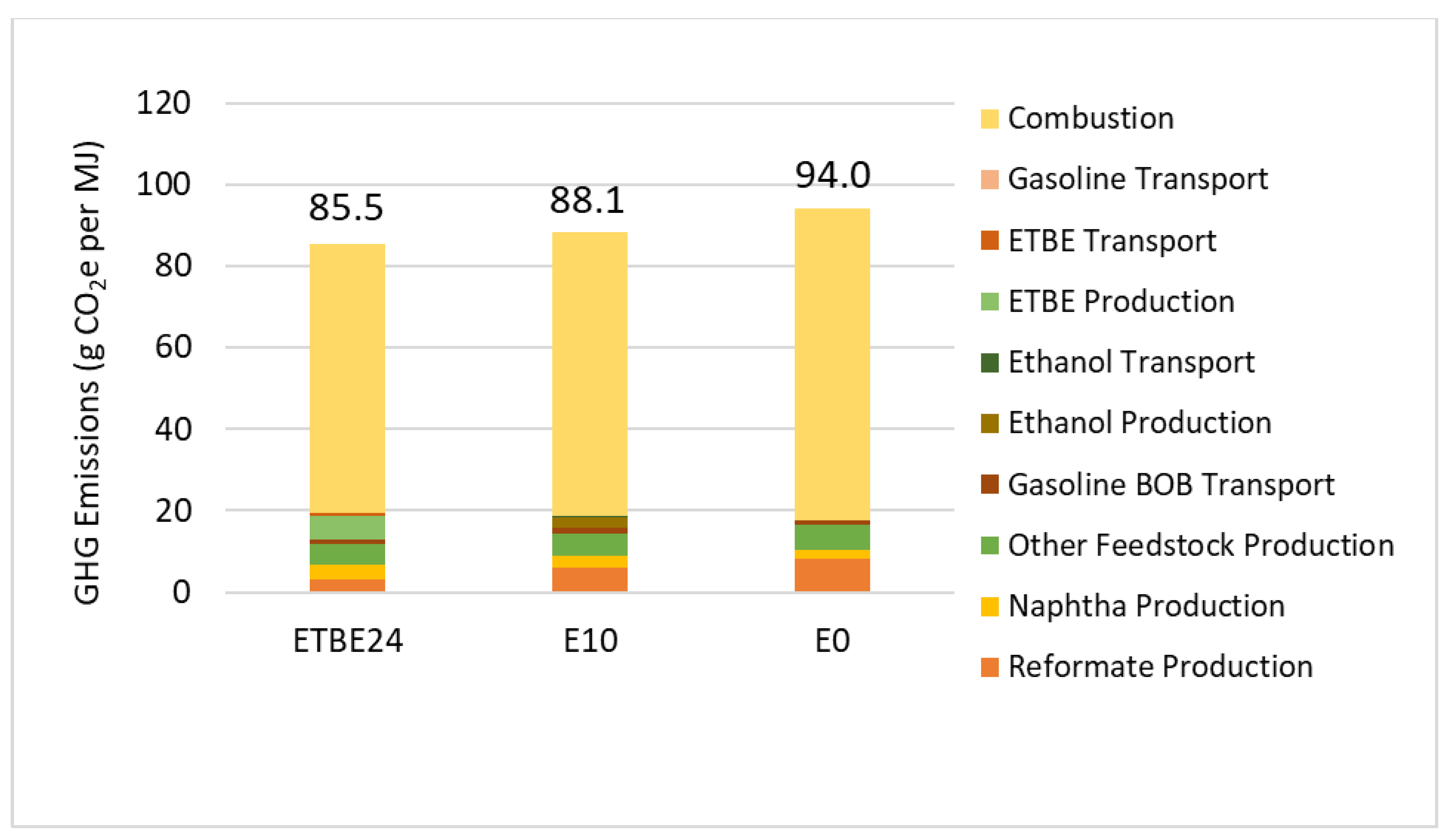
3.2. Country Case Studies

GHG emission results (CO2e per megajoule of energy delivered) for the E0 and the oxygenate blends using solely ethanol or ETBE are presented in Table 8 for the minimum and maximum oxygen levels modeled for each country (complete GHG emission results for all modeled scenarios including intermediate oxygen, mixed ethanol/ETBE blends, and splash blending are provided in Supplemental Data). Results for each country can be compared directly at 3.7% oxygen, with variations in GHG emissions driven by differences in oxygenate sourcing and transport. For Colombia and Japan, at an octane of 89 RON, the replacement of reformate in E0 with an oxygenate to boost octane results in GHG reduction of 6–9 percent. For the higher octane 98 RON scenario in France, GHG reductions for oxygenated fuels range from 7–10 percent. In all of these scenarios, the ETBE blend provides the larger GHG reduction, owing to the higher amount of reformate replaced. The 1.7% oxygen scenarios modeled for Japan and 8.0% oxygen scenarios modeled in France show the trend of lower GHGs as oxygen levels decrease. Japan’s 1.7% oxygen levels show a 3 percent reduction from E0, while the 8.0% oxygen scenarios in France reduce GHGs from 13 percent for the ethanol blend (E23) to 19 percent for the ETBE blend (ETBE51).
Mixed ethanol and ETBE blends presented in Supplemental Data show that GHG reductions track the degree to which the oxygenate volume displaces the reformate. GHG emissions are reduced further relative to ethanol-only blends when ETBE displaces ethanol as an oxygenate, in proportion to the volume of ETBE in the blend. Results for the splash blend case in Colombia, which adds an oxygenate to a base fuel to boost octane unconstrained, suggests that ETBE allows octanes higher than 89 RON to be achieved without GHG penalty.
The GHG emissions for each stage of the lifecycle are shown in Figure 3 for the Colombia 3.7% scenario, and Figure 4 for the France 95 RON 8.0% oxygen scenario (results for all scenarios provided in Supplemental Data). Combustion emissions dominate for all three fuels and are reduced for the ETBE and ethanol blends due to their lower carbon content. The blends using solely ETBE as an oxygenate have the lowest combustion emissions (hence, lower overall emissions) owing to the lower contribution from the reformate. Reformate production emissions drop considerably for the oxygenated fuels that largely displace reformate for octane boost, though these reductions are offset to some degree by larger production emissions for ETBE and ethanol, respectively.

3.3. Sensitivity Analysis

The reported GHG results are driven primarily by the combustion of lower carbon oxygenated fuels rather than modeling inputs for extraction, production, and distribution. Overall results are, therefore, less sensitive to variations in these inputs, but were assessed by analyzing changes in two important scenario assumptions: ethanol feedstock and production location. To show the sensitivity of GHG results to the oxygenate pathway, for the Colombia case study, the 89 RON scenarios were run for all fuels, assuming ethanol was sourced from 100% Colombian sugarcane and 100% U.S. corn (pathway assumptions and results provided in Supplemental Data). In comparison to the primary scenario, the total GHGs vary ± 1 percent because combustion, the largest contributor, is not affected by the ethanol pathway. The variation in non-combustion emissions is roughly ± 5 percent, attributable to ethanol and/or ETBE production. Sugarcane ethanol impacts are lower than those of corn ethanol because sugarcane is a higher-yield agricultural process, is not affected by the same land use change burdens as corn, and it uses bagasse (biogenic source) as the energy input for ethanol processing. An additional sensitivity analysis was performed to remove land use emissions associated with ethanol production. This removal reduces emissions from ethanol and ETBE production by about 10 percent, but since it applies to both oxygenates, it does not affect the relative difference between oxygenated fuel blends.

4. Conclusions

This study provides an updated assessment of lifecycle GHG emissions for ethanol and ETBE-based oxygenated gasolines, based on actual market and policy scenarios in Japan, Colombia, and France. Core to this analysis is the development of new emission factors to improve on published sources such as GREET and ecoinvent with respect to oxygenated fuels. First, a disaggregation of gasoline blendstock allows for the isolation of the energy-intensive gasoline reformate used to boost octane in the absence of an oxygenate. Second, there is the consideration of ETBE production emission factors accounting for the tertiary butyl alcohol (TBA) pathway, updating GREET emission factors from the late 1990s.
Accounting for the variation in emissions among gasoline components and the updated data for ETBE production, this study compared well-to-wheel GHG emissions for oxygenated gasoline blends for a range of oxygen levels including 1.7 wt.% in Japan (current specification), 3.7 wt.% in all three countries (current Colombian and French specifications), and up to 8.0 wt.% in France. Findings are summarized as follows:
  • Results for each country show that adding oxygen to gasoline reduces GHG emissions, and that blends with ETBE produce less GHG emissions than those using only ethanol as an oxygenate;
  • At the common oxygen target of 3.7 wt.%, results from Colombia and Japan at an octane of 89 RON show that the replacement of reformate in E0 with an oxygenate to boost octane results in GHG reduction of 6–9 percent. For the higher octane 98 RON scenario in France, GHG reductions for oxygenated fuels range from 7–10 percent;
  • Relative to E0, the highest well-to-wheel GHG reduction (19 percent) was for a blend of 51% ETBE to achieve 8.0 wt.% oxygen in France, the equivalent of E23;
  • ETBE blends produced GHG reductions that were 38–88% greater than ethanol-only blends at the same oxygen level due to the lower aromatic content required to meet the octane specifications with ETBE blends;
  • Emission reductions from oxygenated fuels were driven in the combustion phase, due to the lower carbon and higher renewable content of ethanol and ETBE blends. The overall GHG reductions are, thus, relatively insensitive to variations in two major upstream inputs, ethanol feedstock and ethanol production country.
These results are rooted in the fundamental principles of carbon balance: at a given octane level, displacing carbon-intensive aromatics with lower-carbon renewable oxygenates reduces GHGs; and using ETBE as an oxygenate rather than ethanol to achieve a target oxygen level lowers GHGs further, even when accounting for its fossil-based portion, because ETBE can be blended at higher volumes. The consistency in GHG reduction for the Colombia, Japan, and France case studies, as well as the Colombia sensitivity case, suggest the GHG reductions are robust and relatively insensitive to the country and source of ethanol. The majority of lifecycle GHG emissions are in the combustion phase; hence, the reductions are driven mainly by renewable oxygenates displacing gasoline aromatics. Current pathways of how renewable oxygenates are produced and transported to the pump are less influential on overall GHG emissions, though the potential to reduce the carbon footprint of oxygenated gasoline further with emerging sources such as cellulosic ethanol and bio-based isobutylene merits further study. The study’s conclusions are, thus, not only directly relevant to Latin America, Asia, and Europe, but can also help advance the state of the science for the selection of oxygenated fuels going forward.
When considering overall GHG emissions across all stages of motor vehicle fuel production, distribution and use, these results (a) support the use of renewable-based oxygenated fuels to reduce carbon emissions; (b) show that using ETBE as an oxygenate provides more GHG benefit than ethanol direct blending at the same renewable content; and (c) demonstrate that reducing aromatic content is central to lowering the carbon footprint of gasoline. The source of ethanol was not found to have an influence on these overall findings. Given the urban air quality impacts associated with the use of low-level ethanol blends, this provides policy makers with additional impetus to re-evaluate the source of an oxygenate in global oxyfuel programs.
This study focused exclusively on greenhouse gas potential, for the reasons identified in the introduction. The impact of oxygenate selection on harmful pollutants and urban air quality has been assessed in previous studies using regional versions of the U.S. EPA MOVES model [38,39]. The authors acknowledge the need for future work that evaluates other environmental impacts relevant to fuels and agriculture, as well as the importance of considering social and economic issues in a broader analysis.

Supplementary Materials

The following supporting information can be downloaded at: https://www.mdpi.com/article/10.3390/fuels5020008/s1, Table S1. GREET land-use parameters; Table S2. GREET land-use parameters; Table S3. Well-to-wheels emission factors by transportation mode; Table S4. Composition of modeled fuel blends for Colombia and Japan; Table S5. Composition of modeled fuel blends for France 95 RON; Table S6. Modeled fuel blends for France 98 RON; Table S7. Colombia Case Study Results; Table S8. Japan Case Study Results; Table S9. France Case Study Results; Figure S1. GHG reduction of oxygenated fuels compared to E0 (France 95 RON); Figure S2. GHG reduction of oxygenated fuels compared to E0 (France 98 RON); Table S10. Pathway inputs (Colombia sensitivity cases); Table S11. Colombia sensitivity analysis results.

Author Contributions

Author contributions for this article were as follows: Conceptualization, S.C., A.D.H. and J.K.; investigation, S.C., B.Y., A.D.H. and J.K.; methodology, B.Y., S.C., A.D.H. and J.K.; software, B.Y. and A.D.H.; validation, B.Y., A.D.H. and J.K.; formal analysis, J.K., B.Y. and A.D.H.; data curation, S.C., B.Y. and A.D.H.; writing—original draft preparation, J.K.; writing—review and editing, J.K.; visualization, B.Y. and J.K.; supervision, J.K. and S.C.; project administration, J.K.; funding acquisition, J.K. All authors have read and agreed to the published version of the manuscript.

Funding

This research was funded by the Latin America Clean Fuels Association (ACELA).

Data Availability Statement

The data presented in this study are openly available within the Global LCA Calculator V4, an MS Excel model constructed to model the scenarios presented. Please contact the corresponding author at john.koupal@erg.com.

Acknowledgments

The authors gratefully acknowledge the significant leadership and technical contribution to this work of Daniel Pourreau of ACELA; Emelyn Chiang of ERG for assistance with data collection and model development; Troy Hottle of Biomason (formerly with ERG) for extracting data from PRELIM and developing a preliminary version of the model expanded on for this work.

Conflicts of Interest

The authors declare no conflicts of interest. The funding entity (ACELA) contributed to the design and scope of the study, with the scope including the publication of results. ETBE production data was provided to the research team by LyondellBasell, a member of ACELA.

References

  1. Anenberg, S.; Miller, J.; Henze, D.; Minjares, R. A Global Snapshot of the Air Pollution-Related Health Impacts of Transportation Sector Emissions in 2010 and 2015; International Council on Clean Transportation: Washington, DC, USA, 2019. [Google Scholar]
  2. Gibbs, L.; Anderson, B.; Barnes, K.; Engeler, G.; Freel, J.; Horn, J.; Ingham, M.; Kohler, D.; Lesnini, D.; MacArthur, R.; et al. Motor Gasolines Technical Review; Chevron Corporation: San Ramon, CA, USA, 2009. [Google Scholar]
  3. Wang, M.; Wu, M.; Huo, H. Life-cycle energy and greenhouse gas emission impacts of different corn ethanol plant types. Environ. Res. Lett. 2007, 2, 24001–24013. [Google Scholar] [CrossRef]
  4. Fazeni-Fraisl, K.; Lindorfer, J. Comparative lifecycle assessment of first- and second-generation bio-isobutene as a drop-in substitute for fossil isobutene. Biofuels Bioprod. Bioref. 2023, 17, 207–225. [Google Scholar] [CrossRef]
  5. van Kasteren, J.M.N. Production of Bioalcohols via Gasification. In Handbook of Biofuels Production, 2nd ed.; Luque, R., Lin, C.S.K., Wilson, K., Clark, J., Eds.; Woodhead Publishing: Sawston, UK, 2016; pp. 495–507. [Google Scholar]
  6. Gomez, L. Colombian Increases Biofuels Blend Mandate to 10%. 2018. Available online: https://apps.fas.usda.gov/newgainapi/api/report/downloadreportbyfilename?filename=Biofuels%20Annual_Bogota_Colombia_7-6-2018.pdf (accessed on 4 January 2024).
  7. Resolución 447 de 2003 Ministerio de Ambiente, Vivienda y Desarrollo Territorial. 2003. Available online: https://ojsrevistaing.uniandes.edu.co/ojs/index.php/revista/article/view/148 (accessed on 19 March 2024).
  8. Wang, M.; Lee, U.; Kwon, H.; Xu, H. Life-Cycle Greenhouse Gas Emission Reductions of Ethanol with the GREET Model. In Proceedings of the Presentation at National Ethanol Conference, Virtual, 16–18 February 2021. [Google Scholar]
  9. Canabarro, N.I.; Silva-Ortiz, P.; Nogueira, L.A.H.; Cantarella, H.; Maciel-Filho, R.; Souza, G.M. Sustainability assessment of ethanol and biodiesel production in Argentina, Brazil, Colombia, and Guatemala. Renew. Sustain. Energy Rev. 2023, 171, 113019. [Google Scholar] [CrossRef]
  10. Beauchet, S.; Guichet, X.; Guyon, O.; Melgar, J.; Pinard, A.; Ternel, C. Study of Greenhouse Gas Emissions from Superethanol-E85 Vehicles in Lifecycle Analysis; IFPEN: Tokyo, Japan, 2022. [Google Scholar]
  11. Yang, Q.; Chen, G.Q. Greenhouse gas emissions of corn–ethanol production in China. Ecol. Model. 2013, 252, 176–184. [Google Scholar] [CrossRef]
  12. Kadam, K.L.; Camobreco, V.J.; Glazebrook, B.E.; Forrest, L.H.; Jacobson, W.A.; Simeroth, D.C.; Blackburn, W.J.; Nehoda, K.C. Environmental Life Cycle Implications of Fuel Oxygenate Production from California Biomass; Report NREL/TP-580-25688; National Renewable Energy Laboratory: Golden, CO, USA, 1999.
  13. U.S. Dept of Energy Argonne National Laboratory. GREET Fuel-Cycle Model. 2021. Available online: https://greet.es.anl.gov/greet_1_series (accessed on 4 January 2024).
  14. Sluder, C.S.; Smith, D.E.; Anderson, J.E.; Leone, T.G.; Shelby, M.H. U.S. DRIVE Fuels Working Group Engine and Vehicle Modeling Study to Support Life-Cycle Analysis of High-Octane Fuels; Oak Ridge National Laboratory Report; US Department of Energy: Washington, DC, USA, 2019.
  15. Croezen, H.; Kampman, B. The impact of ethanol and ETBE blending on refinery operations and GHG-emissions. Energy Policy 2009, 37, 5226–5238. [Google Scholar] [CrossRef]
  16. European Committee on Standardization. European Standardisation on Petroleum and related products. In Proceedings of the 21st International Conference on Renewable Mobility, Berlin, Germany, 22–23 January 2024. [Google Scholar]
  17. U.S. Department of Energy Alternative Fuels Data Center. Global Ethanol Production by Country or Region. Available online: https://afdc.energy.gov/data (accessed on 19 February 2024).
  18. Raj, T.; Chandrasekhar, K.; Kumar, A.N.; Banu, J.R.; Yoon, J.J.; Bhatia, S.K.; Yang, Y.-H.; Varjani, S.; Kim, S.-H. Recent advances in commercial biorefineries for lignocellulosic ethanol production: Current status, challenges and future perspectives. Bioresour. Technol. 2022, 344, 126292. [Google Scholar] [CrossRef] [PubMed]
  19. Agricultural Marketing Resource Center. Cellulosic Ethanol. Available online: https://www.agmrc.org/commodities-products/biomass/cellulosic-ethanol (accessed on 4 January 2024).
  20. Abella, J.P.; Motazedi, K.; Guo, J.; Cousart, K.; Jing, L.; Bergerson, J.A. PRELIM: The Petroleum Refinery Lifecycle Inventory Model, v1.4. 2020. Available online: https://ucalgary.ca/energy-technology-assessment/open-source-models/prelim (accessed on 4 January 2024).
  21. PRELIM Publications. Available online: https://www.ucalgary.ca/energy-technology-assessment/publications (accessed on 8 February 2024).
  22. Gary, J.H.; James, H.H.; Mark, J.K.; David, G. Petroleum Refining: Technology and Economics, 5th ed.; CRC Press: Boca Raton, FL, USA, 2007. [Google Scholar] [CrossRef]
  23. Karonis, D.; Anastopoulos, G.; Lois, E.; Stournas, S. Impact of Simultaneous ETBE and Ethanol Addition on Motor Gasoline Properties. SAE Int. J. Fuels Lubr. 2008, 1, 1584–1594. [Google Scholar] [CrossRef]
  24. Elgowainy, A.; Han, J.; Cai, H.; Wang, M.; Forman, G.S.; DiVita, V.B. Energy Efficiency and Greenhouse Gas Emission Intensity of Petroleum Products at U.S. Refineries. Environ. Sci. Technol. 2014, 48, 7612–7624. [Google Scholar] [CrossRef]
  25. U.S. Dept. of Agriculture. U.S. Biofuels Exports in 2022. Available online: https://fas.usda.gov/data/commodities/biofuels (accessed on 4 January 2024).
  26. Ecoinvent, Ecoinvent v3.7. Available online: https://support.ecoinvent.org/ecoinvent-version-3.7 (accessed on 4 January 2024).
  27. U.S. Dept of Energy National Renewable Energy Laboratory (NREL). U.S. Lifecycle Inventory Database. 2012. Available online: https://www.lcacommons.gov/nrel/search (accessed on 4 January 2024).
  28. IPCC. Climate Change 2013: The Physical Science Basis: Working Group I Contribution to the Fifth Assessment Report of the Intergovernmental Panel on Climate Change; Stocker, T.F., Qin, D., Plattner, G.-K., Tignor, M., Allen, S.K., Boschung, J., Nauels, A., Xia, Y., Bex, V., Midgley, P.M., Eds.; Cambridge University Press: Cambridge, UK; New York, NY, USA, 2013; Available online: https://www.ipcc.ch/report/ar5/wg1/ (accessed on 4 January 2024).
  29. Hamid, H.; Ali, M.A. (Eds.) Handbook of MTBE and Other Gasoline Oxygenates, 1st ed.; Routledge Publishing: London, UK, 2004. [Google Scholar]
  30. Torres, J.; Molina, D.; Pinto, C.; Rueda, F. Study of gasoline mixture with 10% of anhydrous ethanol. Physic-chemical properties evaluation; Estudio de la mezcla de gasolina con 10% de etanol anhidro. Evaluacion de propiedades fisicoquimicas. CTF Cienc. Tecnol. Futuro 2002, 2, 71–82. [Google Scholar]
  31. Anderson, J.E.; Kramer, U.; Mueller, S.A.; Wallington, T.J. Octane Numbers of Ethanol- and Methanol-Gasoline Blends Estimated from Molar Concentrations. Energy Fuels 2010, 24, 6576–6585. [Google Scholar] [CrossRef]
  32. Bourhis, G.; Solari, J.P.; Morel, V.; Dauphin, R. Using Ethanol’s Double Octane Boosting Effect with Low RON Naphtha-Based Fuel for an Octane on Demand SI Engine. SAE Int. J. Engines 2016, 9, 84–98. [Google Scholar] [CrossRef]
  33. Dalli, D.; Lois, E.; Karonis, D. Vapor Pressure and Octane Numbers of Ternary Gasoline–Ethanol–ETBE Blends. J. Energy Eng. 2014, 140, A4014002. [Google Scholar] [CrossRef]
  34. Nikola, R.; Bourhis, G.; Loos, M.; Dauphin, R. Understanding Octane Number Evolution for Enabling Alternative Low RON Refinery Streams and Octane Boosters as Transportation Fuels. Fuel 2015, 150, 41–47. [Google Scholar] [CrossRef]
  35. Junseok, C.; Kalghatgi, G.; Amer, A.; Adomeit, P.; Rohs, H.; Heuser, B. Vehicle Demonstration of Naphtha Fuel Achieving Both High Efficiency and Drivability with EURO6 Engine-Out NOx Emission. SAE Int. J. Engines 2013, 6, 101–119. [Google Scholar] [CrossRef]
  36. Tamour, J.; Nasir, E.F.; Ahmed, A.; Badra, J.; Djebbi, K.; Beshir, M.; Ji, W.; Sarathy, S.M.; Farooq, A. Ignition Delay Measurements of Light Naphtha: A Fully Blended Low Octane Fuel. Proc. Combust. Inst. 2017, 36, 315–322. [Google Scholar] [CrossRef]
  37. Oyekan, S.O. Catalytic Naphtha Reforming Process; CRC Press: Boca Raton, FL, USA, 2018. [Google Scholar] [CrossRef]
  38. Koupal, J.; Palacios, C. Impact of new fuel specifications on vehicle emissions in Mexico. Atmos. Environ. 2019, 201, 41–49. [Google Scholar] [CrossRef]
  39. Noriega, M.; Trejos, E.; Toro, C.; Koupal, J.; Pachon, J. Impact of oxygenated fuels on atmospheric emissions in major Colombian cities. Atmos. Environ. 2023, 308, 119863. [Google Scholar] [CrossRef]
Figure 1. Stages included in analysis (note: transportation included in all stages).
Fuels 05 00008 g001
Figure 2. Individual blendstock GHG emissions (energy basis).
Fuels 05 00008 g002
Figure 3. GHG contribution by lifecycle stage for Colombia 89 RON 3.7 wt.% oxygen scenario.
Fuels 05 00008 g003
Figure 4. GHG contribution by lifecycle stage for France 95 RON 8.0 wt.% oxygen scenario.
Fuels 05 00008 g004
Table 1. Fuel blends included in the case study.
CountryRON0%1.3%2.7%3.7%5.2%6.9%8.0%
Japan89 aE0ETBE8ETBE17E10, ETBE24---
Colombia89 a, 91–96 bE0--E10, ETBE24, E8, ETBE6,
E6, ETBE11,
E5, ETBE13,
E3, ETBE17
---
France95 a, 98 aE0--E10, ETBE24, E5, ETBE13E15, ETBE33,
E10, ETBE11, E5, ETBE22
E20, ETBE44, E15, ETBE11, E10, ETBE22,
E5, ETBE33
E23, ETBE51,
E20, ETBE7,
E15, ETBE18,
E10, ETBE29,
E5, ETBE40
a Match Blend; b Splash Blend; Fuel blend abbreviations: E# = blend with # vol.% ethanol; ETBE# = blend with # vol.% ETBE; E#.ETBE## = blend with # vol.% ethanol, ## vol.% ETBE, and remaining volume gasoline BOB.
Table 2. Pathways for gasoline, ethanol and ETBE by country.
JapanColombiaFrance
Gasoline BOB Production LocationMiddle EastUS Gulf CoastMiddle East
ETBE Production LocationUS Gulf CoastUS Gulf CoastFrance
Ethanol Production Location (Primary)BrazilColombiaFrance
Ethanol Production Location (Secondary)US MidwestUS Midwest-
Ethanol Feedstock (Primary)SugarcaneSugarcaneGlobal mix (sugarcane, corn, beet, wood)
Ethanol Feedstock (Secondary)SugarcaneSugarcane-
Percent of Ethanol from Primary Source55% (ETBE)
100% (Ethanol blends)
55%100%
Gasoline Blending LocationJapanColombiaFrance
Transport of Oxygenate to ConsumerPipeline (ETBE), Truck (EtOH)
Table 3. Properties of “other feedstocks” derived from PRELIM.
ComponentVolume (%)RONMONAromatic (vol.%)
Isopentane3192.690.40
FCC Gasoline3392.678.922.0
HC Gasoline3377.374.70
Alkylate3.493.191.30
Overall10087.681.57.1
Table 4. Default ethanol assumptions in GREET 2021.
Dry Milling w/o Corn Oil ExtractionDry Milling w/corn
Oil Extraction
Wet Milling
Ethanol yield per bushel of corn (gal)2.862.882.67
% of U.S. Production17.7%70.9%11.4%
Table 5. Emissions by stage for oxygenate and gasoline components (g/MJ).
ProductStageLocationCO2CH4N2O
ETBEProduction
(excluding ethanol)
U.S. a12.060.172.4 × 10−4
Europe a14.820.122.0 × 10−4
EthanolCorn ProductionU.S. b7.500.0183.6 × 10−2
Corn Ethanol ConversionU.S. b25.300.0777.3 × 10−4
Sugarcane ProductionBrazil b7.760.0271.8 × 10−2
Sugarcane Ethanol ConversionBrazil b0.300.0346.3 × 10−3
Global Mix ProductionEurope c11.440.0462.1 × 10−2
Ethanol ConversionEurope c15.490.0397.6 × 10−3
Land UseU.S. & Foreign b 7.51-1.6 × 10⁻³
MTBEProductionU.S. b15.780.193.2 × 10−4
ReformateExtraction, ProductionU.S., Middle East d14.140.0961.8 × 10−4
NaphthaExtraction, ProductionU.S., Middle East d8.000.0901.1 × 10−4
Other feedstocksExtraction, ProductionU.S., Middle East d15.780.1092.7 × 10−4
Sources: a New data; b GREET; c ecoinvent; d PRELIM.
Table 6. Fuel component energy, biogenic fraction, and combustion emissions.
ProductLower Heating Value
(btu/gal)
Carbon Content (g/gal)Biogenic
(wt.%)
CO2 (g/MJ)
ETBE102.119844239.1
Ethanol80.51560100-
MTBE98.71914-71.1
Reformate135.12983-81.0
Naphtha123.42333-69.4
Other Feedstocks122.52433-72.8
Table 7. Fuel component oxygen, aromatic and octane properties.
Fuel ComponentDensity (kg/m3)Oxygen
(vol. %)
Aromatic
(vol. %)
Molar Mass
(g/mol)
Octane
(RON)
ETBE74215.7-102.2118.0
Ethanol78934.8-46.1123.0
Reformate866-57.5110.0100.0
Naphtha725--124.864.0
Other feedstocks745-7.1110.087.6
Table 8. Select case study lifecycle GHG emissions (g CO2e/MJ).
Oxygen vol.%:0%1.3%3.7%3.7%8.0%8.0%
Blend:E0ETBE8E10ETBE24E23ETBE51
Japan (89 RON)98.095.393.890.1--
Colombia (89 RON)94.0-88.185.5--
France (98 RON)101.5-93.991.088.681.8
Disclaimer/Publisher’s Note: The statements, opinions and data contained in all publications are solely those of the individual author(s) and contributor(s) and not of MDPI and/or the editor(s). MDPI and/or the editor(s) disclaim responsibility for any injury to people or property resulting from any ideas, methods, instructions or products referred to in the content.

