Stepwise Regression for Increasing the Predictive Accuracy of Artificial Neural Networks: Applications in Benchmark and Advanced Problems

Abstract

A new technique is proposed to increase the prediction accuracy of artificial neural networks (ANNs). This technique applies a stepwise regression (SR) procedure to the input data variables, which adds nonlinear terms into the input data in a way that maximizes the regression between the output and the input data. In this study, the SR procedure adds quadratic terms and products of the input variables on pairs. Afterwards, the ANN is trained based on the enhanced input data obtained by SR. After testing the proposed SR-ANN algorithm in four benchmark function approximation problems found in the literature, six examples of multivariate training data are considered, of two different sizes (big and small) often encountered in engineering applications and of three different distributions in which the diversity and correlation of the data are varied, and the testing performance of the ANN for varying sizes of its hidden layer is investigated. It is shown that the proposed SR-ANN algorithm can reduce the prediction error by a factor of up to 26 and increase the regression coefficient between predicted and actual data in all cases compared to ANNs trained with ordinary algorithms.

1. Introduction

Methodologies based on artificial intelligence (AI) are becoming increasingly common nowadays, with the increase in available computational power and the continuous development of techniques that are constantly improving prediction methods. For example, a large variety of such methodologies are applied in civil engineering for the prediction of structural response; see [1,2,3]. One of the most common machine learning algorithms that are used for the prediction of structural response is the regression artificial neural network (ANN). This model is inspired by the structure and function of the human brain and is capable of solving complex problems that are difficult to solve using traditional rule-based programming techniques. An ANN can perform complex computations on the input data to extract meaningful features and patterns through a large number of interconnected nodes called artificial neurons. These neurons are organized into layers, with each layer performing a specific set of calculations on the input data. The input layer receives the input data, and after the input data are processed through some intermediate hidden layers, the output layer produces the output of the network [4,5].

Many applications of ANNs for predicting structural response exist in the literature. In [6], an ANN hybrid model based on particle swarm optimization (PSO) to predict the maximum surface settlement caused by tunneling is proposed. In [7], an integrated multi-objective harmony search with artificial neural networks (ANNs) is proposed to reduce the high computing time required for the finite-element analysis and the increment in conflicting cost, safety, and corrosion initialization time objectives of post-tensioned concrete box-girder road bridges. A model based on an artificial neural network (ANN) for the prediction of FRP-constrained concrete compressive strength is presented in [8]. In [9], hybrid modeling is proposed to predict the bond strength of glass fiber-reinforced polymer (GFRP) bars to concrete, which is of great significance to the design and implementation of polymer-matrix composites (PMCs) by using the strong nonlinear mapping ability of an artificial neural network (ANN) with the global searching ability of a genetic algorithm (GA). Chatterjee et al. (2017) in [10] proposed a model based on neural network-particle swarm optimization (NN-PSO) to predict the structural collapse of a multistoried reinforced concrete building. Li et al. [11] presented a non-destructive, global, vibration-based damage identification method that utilizes damage pattern changes in frequency response functions (FRFs) and ANNs to identify defects. In [12], an application of ANNs to predict the compressive strength of concrete was presented. Taking the above into account, the importance of ANNs in structural predictions and evaluations becomes apparent.

While artificial neural networks (ANNs) have proven to be highly effective at making predictions across a wide range of applications, there are still several potential problems that can appear during their training or use [13]. The most important such problems are (a) overfitting, i.e., memorizing patterns in the training data with decreased ability to generalize to new data; (b) underfitting, i.e., incapability of the ANN to capture all the patterns in the training data stemming from either data scarcity or reduced complexity of the ANN; (c) vanishing or exploding gradients, which may inhibit the usual learning procedure; (d) lack of interpretability; and (e) increased requirements in terms of computational resources. The severity of the aforementioned issues becomes clear if the difficulties of the training procedure are considered. The training procedure is actually the task of finding the weights and biases of the neurons in the ANN so that it can make accurate predictions by processing input data. This is apparently an optimization procedure. However, the number of design variables in this optimization problem is usually very large, which, given the complexity of the training data and the ANN itself, leads to a highly nonconvex optimization space containing a large number of local minima. This optimization problem is NP-complete, and therefore there does not exist an algorithm to solve the problem of finding an optimal set of weights for a neural network in polynomial time, i.e., learning in neural networks has no efficient general solution [14]. A classical approach to deal with the problem of local minima is to perform random restarts, i.e., train the ANN multiple times with different starting points (random initial weights). This gives some opportunity to the optimization algorithm to find different local minima, and then the better of them are taken as a result [15].

Some usual remedies for the above problems have been the use of regularization during the training process, proper initialization of the network weights and biases, and using more efficient optimization algorithms. Another option is reducing the size of the ANN, i.e., the size and number of its hidden layers. This, apart from reduced overfitting, offers a number of additional advantages, such as faster training, lower memory requirements, reduced complexity, and improved generalization. In light of the above, size reduction should be one of the priorities towards an ANN with minimum training requirements, in a way that ensures that accuracy and predictive ability do not decrease. One first step towards reducing the number of hidden nodes in an ANN while keeping its simplicity is the universal approximation theorem (UAT), which states that an ANN with a single hidden layer can approximate any continuous function (i.e., that two or more hidden layers are not necessary in this case) [16]. It has been demonstrated in that study that finite superpositions of a fixed, discriminatory univariate function can uniformly approximate any continuous function of n real variables with support in the unit hypercube. Continuous sigmoidal functions of the type commonly used in real-valued neural network theory are discriminatory. This implies that one hidden layer comprised of continuous, bounded, nonpolynomial sigmoid transfer functions is enough for ANNs that are developed for the approximation of continuous functions, which is usually the case in engineering applications. The transfer function can be the same for all hidden neurons, and the transfer function of the output layer can be linear. However, the UAT and the relevant literature focus only on its existence without providing any guidelines about the selection of the size (i.e., number of neurons) of the single hidden layer. This is directly related to the precision that is desired for the approximation of an arbitrary continuous function. It has been believed that the required number of neurons inside the hidden layer is relatively large, and this belief becomes stronger if one considers the case of multiple input variables and the associated curse of dimensionality, which makes multidimensional approximation much more computationally demanding, especially for high precision levels. From the above, the importance and advantages of minimizing the training effort of an ANN become obvious. Moreover, the minimization of the training effort of an ANN with a single hidden layer is equivalent to minimizing the size of the latter. However, the size of the hidden layer should not become too low, since in this case underfitting can occur. Therefore, an optimum hidden layer size should be sought.

The present study explores a new approach towards minimizing the size of the hidden layer of regression ANNs in an effort to minimize the computational effort required for their training while maximizing their prediction accuracy. For this purpose, quadratic and cross-product terms of the input parameters are considered additional predictors in the input layer of the ANN. This addition is performed sequentially by using a SR algorithm, which adds or removes the most or least relevant, respectively, from these additional predictors to or from an initial linear regression model based on the statistical criterion of the p value of the F-statistic [17,18]. Thus, in each step, the statistically better of the two regression models (the current model or the model after the addition or removal of the candidate predictor variable) is kept. The SR procedure offers an efficient automatic search procedure that proceeds sequentially, thus avoiding the large computational load associated with other predictor search procedures (e.g., the best subsets algorithm) in cases of a large number of predictor variables [19]. SR avoids the need for the inclusion of all possible $V^2$ quadratic combinations of $V$ inputs which would be clearly infeasible [20]. Also, it gives a definitive answer and does not rely on arbitrary interpretations from the user. An F-test follows an F-distribution and can be used to compare statistical models. The additional quadratic terms are taken into account as additional features in the input training data and thus increase the size of the input layer of the ANN. However, the effect of increasing the input layer on the complexity of the ANN is offset by the reduction in the required size of its hidden layer. It is proven in this study that application of the SR-ANN algorithm not only reduces the required size of the ANN but also reduces the prediction error of the modified ANN (which has its hidden layer size optimized).

The current study is organized as follows. Starting in Section 2 with a motivating example, which involves two elementary classification problems (a linear and a nonlinear), it is proven that, while the linear classification problem can be solved by an ANN without any hidden layers, the nonlinear classification problem requires an ANN with at least one hidden layer to be solved. An ANN without any hidden layers, although unable to solve the nonlinear problem, proves to be able to solve it when SR is applied prior to its training. This constitutes a first observation that the application of SR to the training data can reduce the required number of neurons in the hidden layer or even render it totally unnecessary. Afterwards, the present study proceeds to investigate if the aforementioned ANN size reduction technique can work in cases of realistic datasets. For this purpose, a new methodology, which is presented in Section 3, has been developed to assess the optimum number of neurons in the hidden layer of an ANN. In Section 4, the various components of the SR-ANN algorithm are described, and various aspects of their incorporation into the proposed methodology are elaborated. In Section 5, the accuracy and computational efficiency of the ANNs calculated by the proposed SR-ANN algorithm are tested for four benchmark function approximation problems found in the literature. In Section 6, various distributions of training data of fixed size are considered for training ANNs with varying hidden layer sizes, with or without SR, and useful comparisons are made. After the above, various conclusions are drawn and ideas for future work are formulated.

2. A Motivating Example

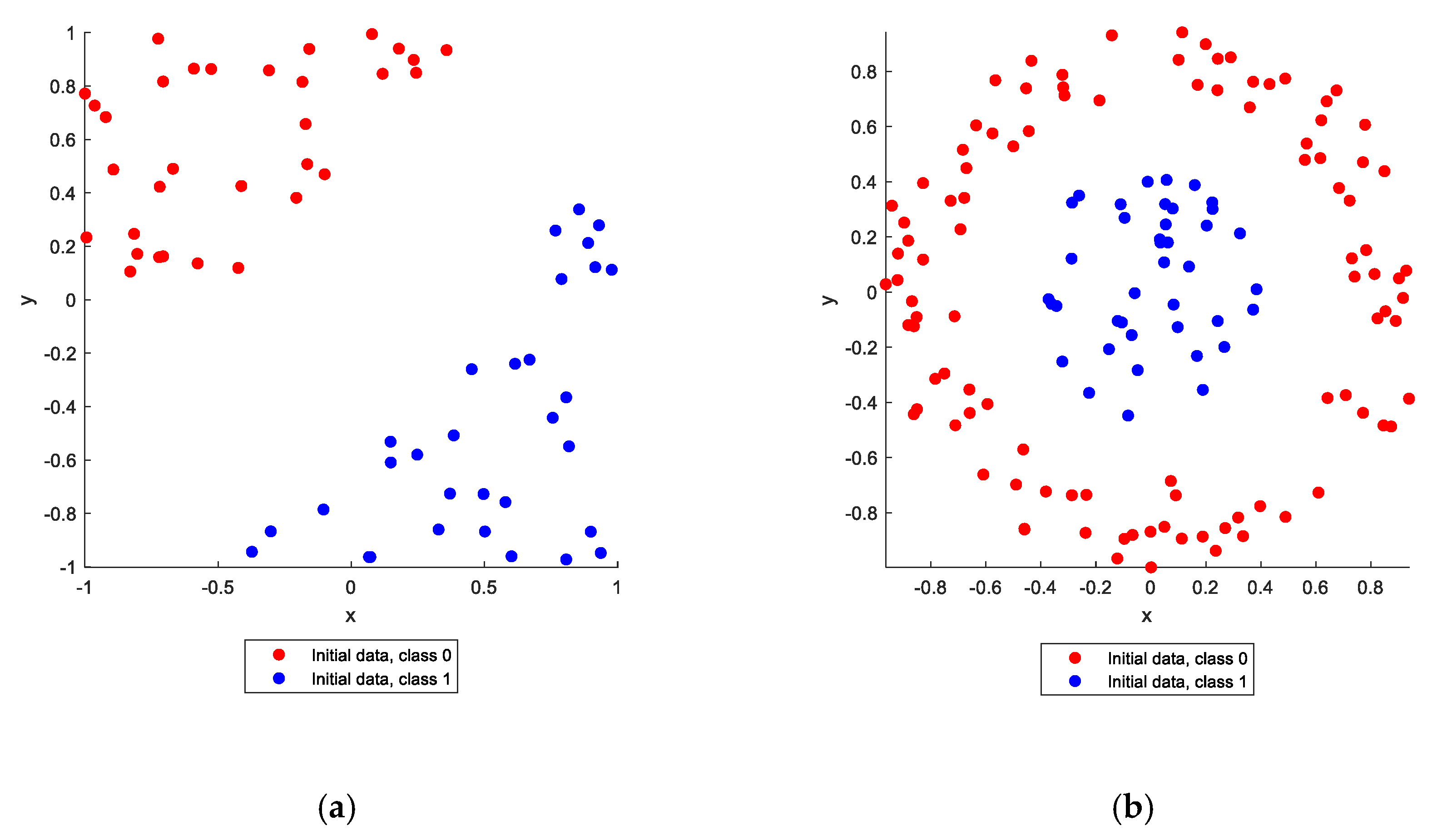
In this section, a visual example of the application of ANNs to solving a classification problem is presented. The purpose of this section is to illustrate how the inclusion of quadratic or other nonlinear functions of the input training data into the training dataset can make the ANN more robust and accurate. Two simple classification problems containing random points in a plane are shown in Figure 1, where the first problem, shown in Figure 1a, is a linear classification problem and the second problem, shown in Figure 1b, is a nonlinear classification problem. Both classification problems involve two different groups of points, labeled “class 0” and “class 1”, in different configurations. In the case of linear classification problems, the separation between the two point groups can be performed with a straight line (or hyperplane in higher dimensions). In the case of nonlinear classification problems, this separation is not possible with a straight line or hyperplane. It is obvious that there is no line that can separate the two point groups in Figure 1b; therefore, any linear regression procedure that could resolve the problem in the linear case cannot work in the nonlinear case, where the application of ANNs or other AI methods for the classification is imperative.

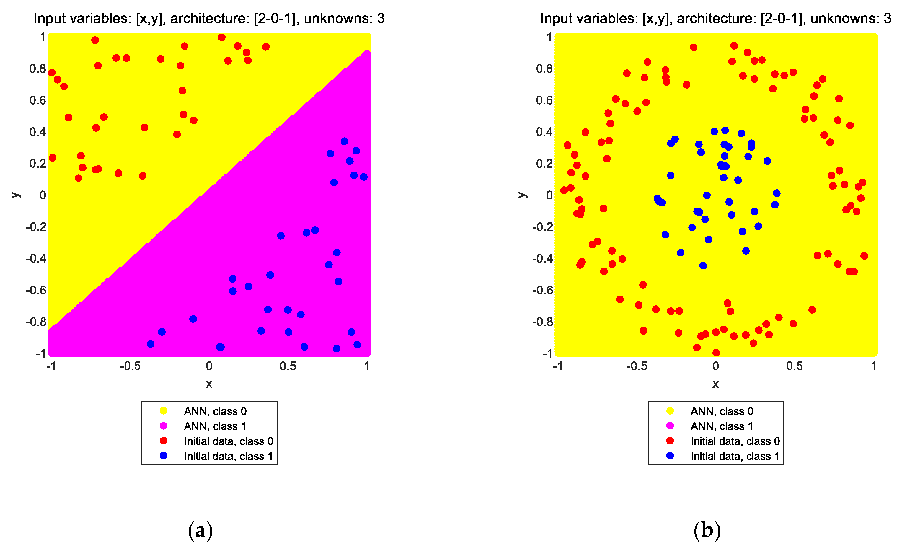
It is well known that an ANN without any hidden layer and with a purely linear transfer function at its output layer acts much like a linear regressor. Such a neural network is applied to the solution of the two classification problems shown in Figure 1. The results are shown in Figure 2a,b, respectively, for the two problems. In the title of each subplot, the input variables, the architecture, and the number of unknowns are noted. The input variables are x and y, denoting the two coordinates of each point in the plane. The architecture is given by the sizes of the input (I), hidden (H), and output (O) layers of the network, in the form of [I-H-O], i.e., starting from the input layer towards the output layer. The notation [2-0-1] means that the ANN has an input layer of size 2 (two neurons) and an output layer of size 1 (one neuron), whereas it does not have any hidden layers. The number of unknowns is the number of independent design variables of the ANN that need to be calculated through the training process; as this number increases, the computational effort required for the optimization process increases as well. It is obvious that this type of ANN, while able to solve the linear classification problem (note the decision boundary along the line where the color changes in Figure 2a), cannot solve the nonlinear classification problem and erroneously assigns the label “class 0” to all points, thinking that all points belong to a single group (Figure 2b).

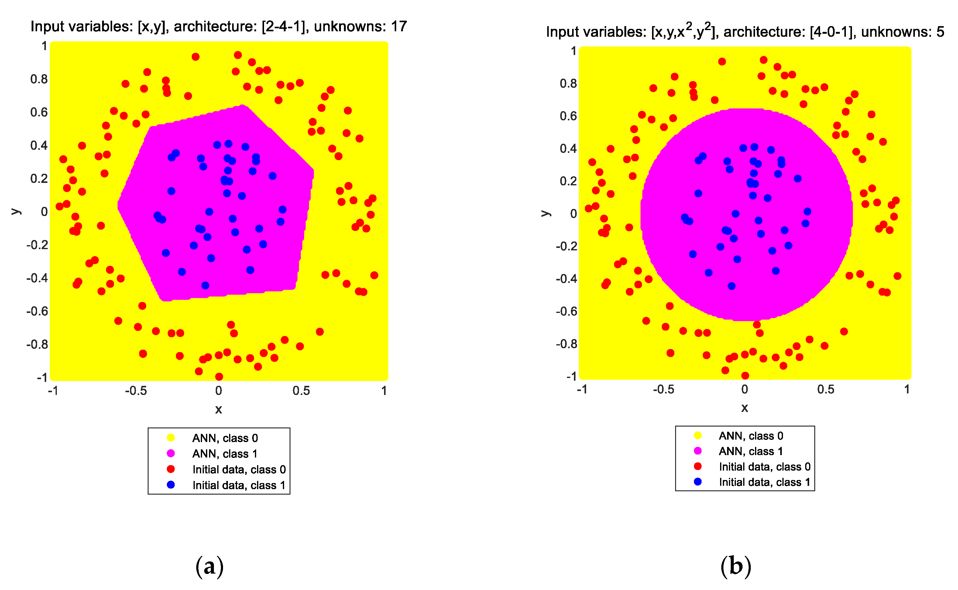
How can one proceed from this point to solve the nonlinear problem? There are two options: either (a) increase the size of the ANN, which is the usual way to tackle underfitting phenomena like the one at hand, or (b) include nonlinear terms in the input data, which can be performed either manually or automatically through a SR procedure or other similar methods. The central idea of this study is to examine which of these two options is better to follow for developing regression ANNs used for engineering purposes. The results of the two aforementioned options are shown in Figure 3a,b, respectively.

The region of the plane in yellow is perceived by the ANN as class 0, whereas the region in magenta is perceived as class 1. The solution is considered correct if all “class 0” initial points belong inside the “class 0” region as perceived by the ANN; the same applies for the “class 1” initial points and region. Both approaches seem to solve the classification problem since it is obvious that the two point groups are placed into the respective areas of the plane. i.e., the red points are inside the yellow region (class 0), and the blue points are inside the magenta region (class 1). However, one has to notice the large difference in the computational demands of the two approaches. In the first option, it was found that a hidden layer of at least four neurons is required, whereas in the second option, no hidden layer is required at all, but the size of the input layer has increased from two to four by adding the quadratic terms (see the architectures noted in the titles of Figure 3a,b, respectively). This difference is apparent in the number of unknowns as well, which is 17 for the ANN with the hidden layer and only five for the ANN without the hidden layer, despite the larger input layer size of the latter. It is obvious that one should select the latter approach to solve the problem. But is this a general trend that could be applied to regression ANNs in general? This issue will be addressed in the next sections.

3. Proposed Methodology for Optimizing the ANN Architecture

3.1. Workflow of the Proposed Methodology

In Figure 4, the workflow of the proposed methodology is shown. The various processes involved in this workflow are indicated by blue arrows, whereas the starting and ending points of each process are indicated by red circles. There are four main phases in this workflow:

• Normalization (division by the maximum absolute value, or mapping to the interval [0, 1]) or standardization (linear transformation such that mean value and standard deviation become 0 and 1, respectively) of the training data, i.e., the mean value of each input variable is subtracted and the result is divided by the standard deviation, so that all observations of each variable are reduced to the standard normal distribution of the corresponding variable.
• SR of the input data to obtain an optimized regression model, according to the theory presented in Section 4.1 of the present study.
• Enhancement of the training data by adding the quadratic terms that exist in the formula of the regression model, which is obtained after the SR procedure of the previous step.
• Training of the ANN with the BR algorithm using k-fold cross validation, according to Section 3.2 of the present study.

3.2. Description of the Algorithm for Parametric Analysis

In this section, the final step of the flowchart presented in Figure 4, and more specifically, the 10-fold validation procedure, is explained in more detail. As is mentioned in the introduction section, the size of the hidden layer of the ANN should not become too low, since in this case underfitting can occur, i.e., the ANN reaches a state where it cannot capture enough patterns in the training data. On the other hand, the hidden layer size should not become too large, since in this case overfitting can occur, i.e., the ANN memorizes patterns in the training data with a decreased ability to generalize to new data. For an ANN with an input layer of size $I$, a single hidden layer of size $H$, and an output layer of size $O$, the number of parameters (weights and biases) $N_w$ to be determined during training is given by the following:

$$N_w=\left(I+1\right)H+\left(H+1\right)O.$$

(1)

In addition to this, in the context of a training dataset, each one of the $N$ observations in the dataset contributes to a set of $O$ training equations, where the input variables are used to predict the output variables. Therefore, the total number of training equations is equal to the following:

$$N_{trneq}=NO.$$

(2)

It is obvious that the number of parameters in the ANN should be lower than the number of training equations in the training dataset to avoid indeterminacy:

$$N_w<N_{trneq}.$$

(3)

Substitution of Equations (1) and (2) into (3) yields the following upper limit for the hidden layer size $H$ (overfitting limit):

$$H<\frac{\left(N-1\right)O}{I+O+1}=n_H.$$

(4)

In the present study, $O=1$, and the inequality (4) becomes the following:

$$H<\frac{N-1}{I+2}=n_H.$$

(5)

Apart from the above, it is apparent that $H$ cannot be lower than 1 (underfitting limit). Therefore, the valid range for $H$ is $1<H<n_H$. The two aforementioned unfavorable cases imply that there is a point in between the two extremes that will minimize the effect of both, i.e., that there is an optimum value of $H$, between 1 (underfitting extreme) and $n_H$ (overfitting extreme), which will maximize the predictive accuracy of the ANN. Scanning the interval $\left[1,n_H\right]$ through a parametric analysis, which is performed in the final step of the flowchart shown in Figure 4 (“Parametric analysis of varying ANN size”), reveals the optimum value of $H$, and therefore the proposed method has the potential to enhance the optimal hidden layer size of ANNs. The aforementioned trends for $H$ hold regardless of whether SR is applied or not. In addition to this, it is expected from Inequality (5) that the upper limit for the hidden layer size $n_H$ decreases when SR is applied, since the latter increases the size of the input layer $I$. This offers additional benefits because it further limits the range of variation of $H$, leading to reduced computational effort for the parametric analysis at the final step of the flowchart shown in Figure 4. $n_H$ can be either defined using Equation (4) or appropriately selected by the user to avoid excessive computational effort. In the present study, $n_H=15$ has been specified for all cases, with the optimum hidden layer size being lower than this number for all cases examined.

The k-fold cross-validation technique is used to estimate the prediction skills of the ANNs that are developed in this study. This approach involves randomly dividing the set of observations into k groups, or folds, of approximately equal size. Each group is treated as a validation set, and the ANN is fit on the remaining $k$ − 1 folds [21]. Ten-fold cross-validation is used in this study. For each value of hidden layer size, the training dataset is randomly separated into 10 groups (folds). For each one of these folds $n_r$, ANNs are trained with random initialization of their weights in each restart, where, in the present study, $n_r=5$. The validation error of these $n_r$ ANNs is calculated, and the $n_{excl}$ worst ANNs are excluded from the calculation to avoid any cases of nonconvergent ANNs with high performance errors that could disproportionately affect the results. $n_{excl}=2$ in the present study. For each number of neurons in the hidden layer of the ANN, the mean values of the training and validation performance error and regression are calculated among 30 ANNs (10 folds × 3 ANNs per fold). Finally, the aforementioned mean values are monitored throughout the parametric analysis. Algorithm 1 shows the flowchart of the procedure described above.

Algorithm 1 Flowchart of parametric analysis

1: $\mathrm{for} H$$\mathrm{from} 1 \mathrm{to} n_H$ (hidden layer sizes) 2:   Define k folds in training data 3:   $\mathrm{for} i$ from 1 to k (folds) 4:     $\mathrm{Define} \mathrm{the} \mathrm{training} \mathrm{data} \left[X_{tr},Y_{tr}\right]$ containing all folds except for the $i^{th}$ fold 5:     $\mathrm{Define} \mathrm{the} \mathrm{validation} \mathrm{data} \left[X_{val},Y_{val}\right]$$\mathrm{as} \mathrm{the} i^{th}$ fold 6:     $\mathrm{for} j$$\mathrm{from} 1 \mathrm{to} n_H$ (ANNs) 7:         $\mathrm{Train} \mathrm{the} j^{th}$$\mathrm{ANN} \mathrm{with} \left[X_{tr},Y_{tr}\right]$ as training data 8:         $\mathrm{Evaluate} {MSE}_{tr,H,i,j}$$\mathrm{and} {MSE}_{val,H,i,j}$$\mathrm{for} \left[X_{tr},Y_{tr}\right]$$\mathrm{and} \left[X_{val},Y_{val}\right]$ respectively 9:         $\mathrm{Evaluate} R_{tr,H,i,j}$$\mathrm{and} R_{val,H,i,j}$$\mathrm{for} \left[X_{tr},Y_{tr}\right]$$\mathrm{and} \left[X_{val},Y_{val}\right]$ respectively 10:     end for 11:     $\mathrm{Sort} {MSE}_{val,H,i}$ in ascending order 12:     $\mathrm{Delete} \mathrm{the} \mathrm{ANNs} \mathrm{corresponding} \mathrm{to} \mathrm{the} n_{excl}$$\mathrm{largest} \mathrm{values} \mathrm{of} {MSE}_{val,H,i}$ 13:     $\mathrm{Update} {MSE}_{tr,H,i}$$, {MSE}_{val,H,i}$$, R_{tr,H,i}$$\mathrm{and} R_{val,H,i}$ after the deletion of step 12 14:  end for 15:  $\mathrm{Take} \mathrm{the} \mathrm{mean} \mathrm{values} \mathrm{of} {MSE}_{tr,H}$$, {MSE}_{val,H}$$, R_{tr,H}$$\mathrm{and} R_{val,H}$ 16: end for 17: Select the ANN with the minimum testing error.

4. SR Applied to ANNs

4.1. SR Procedure

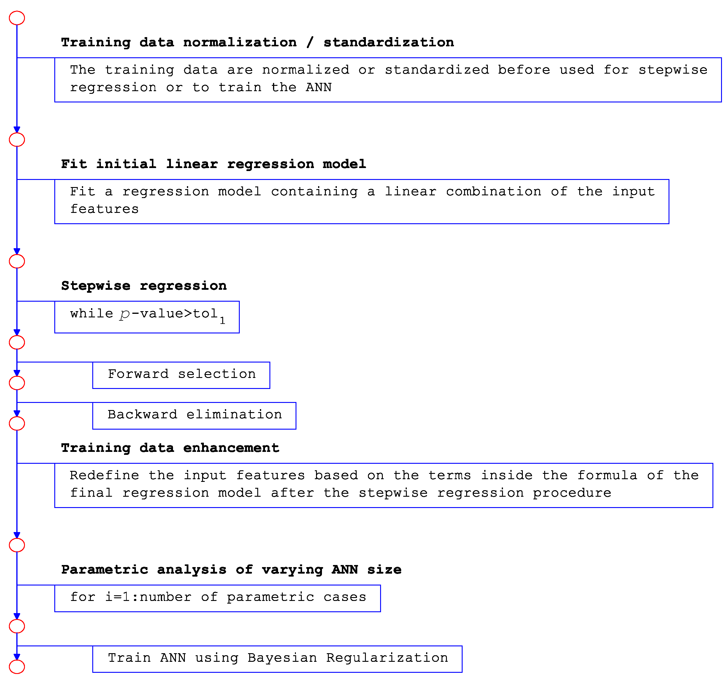
SR is a method that adds and removes terms from an initial regression model (which in this study is considered to be linear) based on their statistical significance in explaining the response variable in a number of steps. It is virtually a stepwise model selection procedure, and it can handle terms that are nonlinear functions of the initial features. The following procedure is followed in order to arrive at the final regression model:

• Fit an initial linear regression model of the form:

$$y_{init}=a_0+\sum _{n=1}^k{a}_n{x}_n.$$

(6)

The residuals of the fitted regression model generally follow a nearly normal distribution. Training data that correspond to outliers of this distribution can be removed or not. In the present study, outliers are not removed.

2.

Apply forward stepwise selection by examining a set of available terms that do not belong to the model and have p-values of the F-statistic less than an entrance tolerance (that is, if it is unlikely that a term would have a zero coefficient if added to the model). Among the above terms, the term with the smallest p-value is added to the model, and the procedure is repeated; otherwise, proceed with step 3 below. The F-statistic is computed as follows:

$$F=\frac{\frac{{SS}_i-{SS}_{i+1}}{{df}_i-{df}_{i+1}}}{\frac{{SS}_{i+1}}{{df}_{i+1}}},$$

(7)

where ${SS}_i$ is the residual sum of squares for the current model (iteration $i$) and ${SS}_{i+1}$ is the residual sum of squares for the next model (iteration $i+1$). There are $df=N-V$ degrees of freedom, where $N$ is the number of data observations (or, equivalently, the training data size), $V$ is the number of predictors being estimated (one degree of freedom is lost per predictor estimated), and ${df}_i$, ${df}_{i+1}$ are the degrees of freedom of the current and next model respectively. The p-value is then calculated based on the F cumulative distribution function of the F-statistic of Equation (7):

$$p=1-I_{{df}_{i}x/\left({df}_{i}x+d{f}_{i+1}\right)}\left(\frac{{df}_i}{2},\frac{{df}_{i+1}}{2}\right),$$

(8)

where $I$ is the regularized incomplete beta function given by the following:

$$I_x\left(a,b\right)=\frac{{\int }_0^x{t}^{a-1}{\left(1-t\right)}^{b-1}dt}{{\int }_0^1{t}^{a-1}{\left(1-t\right)}^{b-1}dt}.$$

(9)

3.

Apply backward stepwise selection by examining if any of the available terms in the model have p-values greater than an exit tolerance (that is, the hypothesis of a zero coefficient cannot be rejected). Among the above terms, remove the term with the largest p-value and return to step 2; otherwise, end the process. In Equations (7)–(9) above, it is considered that the next model (iteration $i+1$) is more complex than the current model (iteration $i$) and the same holds for the backward stepwise selection step, in which the calculation of the F-statistic and the p-value is made according to the same equations as above.

In this study, it is assumed that the largest set of terms in the final model contains an intercept term, linear and squared terms for each predictor, and all products of pairs of distinct predictors as follows:

$$y_{SR}=a_0+\sum _{n=1}^k{a}_n{x}_n+\sum _{n,m=1}^k{a}_{n,m}{x}_n{x}_m.$$

(10)

In addition, the entrance and exit tolerances are set equal to 0.05 and 0.10, respectively. Of course, these selections can be modified depending on the complexity of the training data, which is regressed. A more detailed description of the SR procedure can be found in Section 6.1.2 of [22]. SR has already been applied for the prediction of the load resistance of longitudinally stiffened webs subjected to patch loading [23]. However, the last study did not involve any ANNs for making predictions. To the best of the author’s knowledge, no study up to date has exploited this technique to increase the predictive ability of ANNs.

4.2. Artificial Neural Network Properties

The ANNs that are involved in the present study are feedforward networks with the following characteristics:

• A Bayesian regularization (BR) algorithm is used as the training function. This algorithm, instead of merely minimizing the squared errors, minimizes a linear combination of squared errors and weights during the training of the ANN within the Levenberg–Marquardt algorithm. This linear combination is appropriately modified in order to achieve good generalization properties of the ANN [24,25]. Training stops when the performance error minimizes to zero, or the performance gradient becomes lower than 1 × 10⁻⁷, or when the Marquardt adjustment parameter becomes larger than 1 × 10¹⁰, whatever occurs first. It has been generally accepted that BR ANNs avoid overfitting without the need for validation sets during training because the regularization pushes unnecessary weights towards zero, effectively eliminating them [26]. Due to these advantages, BR has been selected as the training algorithm for ANNs in the present study through the option net.trainFcn = ‘trainbr’ in Matlab R2022b.
• Mean squared error (MSE) is used as the performance function. For $k$ observations with actual values $y_{n,actual}$ and predicted values $y_{n,pred}$, this error is given by the following equation:

$$MSE=\frac{{\sum }_{n=1}^k{\left(y_{n,pred}-y_{n,actual}\right)}^2}{k}.$$

(11)

The corresponding option in Matlab is net.performFcn = ‘mse’.

• The hyperbolic tangent sigmoid (tansig) function is used as a transfer function from the input to the hidden layer, and the linear function (purelin) is used as a transfer function from the hidden layer to the output layer. These functions are given by the following formulae:

$$tansig\left(x\right)=\frac{2}{1+e^{-2x}}-1$$

(12)

$$purelin\left(x\right)=x .$$

(13)

It is noted that the derivative of the $tansig$ function is noticeably larger and smoother than the derivatives of other (sigmoid) functions near zero. This enables the training algorithm to find the local or global optima of the ANN weights and biases, i.e., to minimize the cost function, faster [27]. The transfer functions are defined by the options:

net.layers{1}.transferFcn = ‘tansig’

net.layers{2}.transferFcn = ‘purelin’

for the hidden and output layers, respectively.

• The datasets used for the development of the ANNs in this study are divided into a design data set (90% of the total data used for training purposes) and a test data set (10% of the total data used for the 10-fold validation process). The entire design data set mentioned above (i.e., 90% of the total) is used for training purposes of the ANN without any validation or testing data. The explanation behind this selection is that early stopping through a check of the number of validation failures is not used (since regularization is used in the trainbr function), and therefore any validation data would be useless. In addition, testing data have already been assigned (see 10% above), and therefore there is no need to use testing data during the training process. The aforementioned points have been materialized by the following selections in Matlab:

net.divideFcn = ‘dividerand’

net.divideMode = ‘sample’

net.divideParam.trainRatio = 100/100

net.divideParam.valRatio = 0/100

net.divideParam.testRatio = 0/100

net.trainParam.epochs = 1000

net.trainParam.max_fail = a

The last two options ensure that validation failure does not occur within the maximum number of training epochs, when a > 1000.

For more details about the various Matlab commands presented above, the reader is referred to the Matlab help section [28].

4.3. SR as Both a Data Augmentation and ANN Configuration Tool

Any regression model that accepts training data that are enhanced through a SR procedure contains the features or feature combinations that are supposed to have the most control over the output dependent variable(s), by definition of the SR algorithm. In addition to this, data augmentation for regression problems typically involves techniques that introduce variability in the input data while preserving the output values. One of these techniques, among others, is the feature engineering process, in which new input features are created from existing ones. This can help to increase the diversity of the input data and improve the ANN’s ability to learn complex relationships between the input and output variables. From the aforementioned points, it can be assumed that the SR process plays the role of feature engineering or, more broadly, a data augmentation tool. On the other hand, it should be noted that the SR process, apart from augmenting the training data, simultaneously configures the subsequently trained ANN, in the sense that it directly determines the size of its input layer and indirectly determines the prediction power of the ANN. This implies that the SR procedure adds some kind of knowledge to the trained ANN, i.e., it directly influences the training process. Therefore, in the context of the present study, it is difficult to make a clear distinction between the two effects of SR as a data augmentation or ANN configuration tool. Maybe both of them apply, more or less. The aforementioned points justify the need for integrating the SR process with ANNs towards the development of more robust prediction tools.

4.4. Integrating SR with ANNs: Why Are the Two Expected to Complement Each Other?

Both stepwise regressors and ANNs are tools intended for regression tasks. However, there are some characteristics in which the two could complement each other, and therefore their integration yields a robust prediction scheme. The most significant differences between stepwise integration and ANNs are the following:

• Nonlinearity is taken into account in different ways in the two methodologies. Namely, in SR, nonlinearity stems from the inclusion of nonlinear features in the data, whereas in ANNs, nonlinearity stems from the transfer functions.
• The amount of training data that is required or that can be handled. For small amounts of training data, SR methods can perform better predictions, whereas ANNs are susceptible to overfitting. For large datasets, common regression methods may struggle due to their decreased adaptability, whereas ANNs can be easily trained, and their predictive power increases.
• Interpretability: ANNs are mostly viewed as black boxes due to the obscure processes that they use to make predictions. This implies that, in the case of a prediction error, it is hard to trace its source and fix it. On the contrary, integrating the ANN with an SR procedure reduces its complexity and obscurity by shifting its computational power from the hidden layer(s) to the input layer. Since the input layer accepts data actually observed or recorded in nature, it is better conceivable for humans, and therefore controlling the respective ANN becomes an easier task.

In this study, the two computational models are used in series; using them in parallel or in combination with other regression models is an open subject for further research.

5. Testing the Proposed SR-ANN Algorithm for Benchmark Function Approximation Problems

In this section, the approximation accuracy of the ANNs, the architecture of which is optimized according to the proposed SR-ANN algorithm, is tested for a number of benchmark problems.

5.1. Approximation to cos(x)

A simple trigonometric function is selected to test the approximation performance of the SR-ANN algorithm. The training data for this problem consist of 222 uniformly chosen points in the interval $\left[0,\mathsf{\pi }\right]$ and the outputs are equal to the function $\mathrm{y}=\left(\mathrm{c}\mathrm{o}\mathrm{s}\left(2\mathrm{x}\right)+1\right)/3$. This formula has been specifically selected to keep the output range between 0 and 1. Of the 222 training points, 200 are used for training, and 22 are used for the 10-fold validation of the proposed ANNs ($22\cong 222/10$). The approximation results are presented in terms of the relative approximation error, defined as $\left({\mathrm{y}}_{\mathrm{A}\mathrm{N}\mathrm{N}}-{\mathrm{y}}_{\mathrm{E}\mathrm{X}\mathrm{P}}\right)/{\mathrm{y}}_{\mathrm{E}\mathrm{X}\mathrm{P}}$, as a function of the input values. The ANN is considered to have two hidden neurons, according to [29]. Following this option, the proposed SR-ANN algorithm is applied to train an ANN with two hidden layers. The relative errors achieved in [29] and by the SR-ANN algorithm are compared in Figure 5. It is observed that the maximum error of the proposed method is equal to 0.19%, whereas the maximum error of [29] is 5.5%, which is about 30 times larger. From the legend of Figure 5, it is apparent that the SR procedure has added a quadratic term of the input variable as a feature in the input training data of the ANN, the final architecture of which is [2-2-1]. In addition, it is observed that in the approximation of the considered function, singularities occur at π/2 for the method proposed in [29] and at π/4 and 3π/4 for the proposed SR-ANN algorithm. This difference is attributed to the different transfer functions that are used in the two different cases.

In addition to the above, it is useful to present the optimal ANN architecture that the proposed SR-ANN algorithm gives for the above approximated function. The performance MSE error and regression coefficient between the predicted and actual output data are shown in Figure 6 for this case. It seems that the optimum size of the hidden layer, which corresponds to the minimum testing error, is found to be 14, whereas it is obvious that the regression coefficient is practically close to unity for all cases of hidden layer size larger than 1. The relative error of the ANN with the optimized architecture as above is shown in Figure 7. By comparing the results of Figure 5 and Figure 7, it is found that the error of the ANN with optimum architecture [2-14-1] is about 0.05%, whereas the error of the ANN with architecture [2-2-1] is roughly 0.19%, which is approximately 4 times higher. In this example, the capability of the proposed SR-ANN algorithm to provide ANNs with a very close approximation to a trigonometric function is evident. In the following, more benchmark examples will be considered to obtain a more general picture.

5.2. Approximation to Gamma Function

The gamma function is given by the following equation:

$$\Gamma \left(z\right)={\int }_0^{\infty }{t}^{z-1}{e}^{-t}dt.$$

(14)

The gamma function has been approximated with an ANN using the proposed SR-ANN algorithm. According to reference [29], the input variable in the training dataset ranges between 0 and 20, and the output of the function approximated by the ANN is given by $ln\left(\Gamma \left(z\right)\right)$, in order to avoid overflow problems. In addition, 1111 points have been included in the training dataset, of which 90% (i.e., 1000) are used for the training phase and the remaining 111 points are used for the 10-fold validation process. The performance MSE errors for the training and testing datasets are shown in Figure 8. In this figure, it is apparent that application of the SR-ANN algorithm leads to lower values of error compared to the same procedure without SR applied. According to the findings of the SR-ANN algorithm, the optimum architecture of the ANN is 12, and the corresponding testing error is 9 × 10⁻⁸.

In reference [29], the ANN is considered to have 20 hidden neurons. This case has also been solved with the proposed SR-ANN algorithm. The relative error of the ANNs for the approximation of the gamma function as described above is shown in Figure 9. It is obvious that the proposed SR-ANN algorithm results in an ANN with superior accuracy since the maximum relative error according to [29] is about 0.65%, whereas according to the proposed SR-ANN algorithm it is about 0.1% (approximately 6.5× lower) as shown in Figure 9.

In Figure 10, the relative error of the ANN with the optimum architecture according to the SR-ANN algorithm is shown. The maximum error is about 0.4%, a value that is a little lower than that of [29]. However, the architectures of the ANNs are substantially different, where the ANN in [29] has 20 hidden nodes whereas the ANN involved in Figure 10 has 12 nodes. This fact has certain implications regarding the required computational effort to train the two ANNs. It is therefore shown that the proposed SR-ANN algorithm can lead to computationally lighter ANNs, achieving roughly the same accuracy as the ANN trained with ordinary methods.

5.3. Approximation to the Upper Tail Integral of the Gauss Distribution Function

The complimentary error function, $erfc\left(x\right)$, is defined by the following equation:

$$erfc\left(x\right)=\frac{2}{\sqrt{\pi }}{\int }_x^{\infty }{e}^{-t^2}dt.$$

(15)

In [29], an ANN with architecture [1-20-1] is used, and the upper tail integral of the Gauss distribution is used for approximation by the ANN. The upper tail integral is defined by the following:

$$Q\left(x\right)=\frac{1}{2}erfc\left(\frac{x}{\sqrt{2}}\right).$$

(16)

The input variable ranges between 0 and 20, and the output corresponds to $ln\left(Q\left(x\right)\right)$. Similar to the gamma function, 1111 points are considered for training and validation of the ANNs, for which 10-fold validation is performed. In the case of varying the hidden layer size of the ANN, the performance MSE error for the training and testing datasets by applying the proposed SR-ANN algorithm is shown in Figure 11. It is observed in this figure that the testing error of the ANN when the proposed SR-ANN algorithm is applied is generally lower than the case in which SR-ANN is not applied, except for the case of a hidden layer size equal to 3. The optimum ANN architecture is found to be equal to 6 hidden neurons, whereas the corresponding error is roughly equal to 3.5 × 10⁻¹¹.

In addition to the above, the ANN with 20 hidden nodes has been trained using the proposed SR-ANN algorithm, and the relative error results are compared to the relative error results of [29]. These results are shown in Figure 12. It is observed that the maximum error of [29] is roughly equal to 0.3%, whereas the maximum error of the proposed method is 0.1%, which is approximately 3 times lower than the former. Therefore, it is shown that the suggested SR-ANN algorithm can produce ANNs more accurately than those trained with usual methods. The relative error of the ANN with optimized architecture, according to the proposed SR-ANN algorithm, is shown in Figure 13. The maximum error in Figure 13 is around 0.0025%, which is lower than both errors observed in Figure 12. This implies that a higher number of hidden neurons in an ANN is not always beneficial for its accuracy, since the ANN involved in Figure 13 has only 6 hidden neurons, whereas the ANNs involved in Figure 12 have 20 hidden neurons. It is apparent that in this case, the proposed SR-ANN algorithm achieves simultaneously lower computational effort, accompanied by better accuracy.

5.4. Approximation to the Sphere Function

In reference [30], the sphere function of two variables has been considered a benchmark function in order to test the approximation capabilities of various types of ANNs proposed in that study. The sphere function is defined as follows:

$$f\left(x\right)={\sum }_{i=1}^2{x}_i^2.$$

(17)

where the two variables $x_1$ and $x_2$ range between −100 and 100, at a step of 10. The performance MSE error for the training and testing datasets by applying the proposed SR-ANN algorithm for approximation of the sphere function is shown in Figure 14. It is apparent that the optimum ANN has five hidden neurons and exhibits a testing error roughly equal to 0.0002. The best MSE result shown in Table 2 of [30] among the three different ANNs considered in that study is 0.1793 and corresponds to the back propagation algorithm. By comparing the two aforementioned MSE values, it becomes evident that the proposed SR-ANN can yield ANNs with superior accuracy compared to ANNs trained with conventional methods. It is also concluded from Figure 14 that the ANNs generated by applying the SR-ANN algorithm demonstrate lower values of error compared to the ANNs for which the SR-ANN algorithm is not applied. Moreover, it is noted that since four different (unrelated) function approximation problems are considered in Section 5.1, Section 5.2, Section 5.3 and Section 5.4, the performance MSE error ranges of Figure 6a, Figure 8a, Figure 11a, and Figure 14a cannot be directly compared.

6. Effect of SR on ANN Performance for Multivariate Problems with Various Data Sizes and Distributions

It is of interest to investigate the predictive behavior of an ANN with and without SR for various training datasets. In this way, a first assessment of the accuracy and robustness of the proposed methodology in data encountered in realistic engineering problems will be made. Furthermore, since in engineering applications there is usually scarcity in experimental cases due to technical infeasibility, economics, or other reasons, it is of interest to see the aforementioned behavior for datasets of relatively small size. Typical sizes of training data that are used for ML applications for making predictions in engineering practice are given in

Table 1. Size and number of variables of typical datasets used for ML applications in civil engineering.

Number of Input Variables	Number of Samples	Application	Reference
5	285	Shear resistance of reinforced masonry shear walls	[32]
5	1017	Axial compressive strength of CFST columns	[33]
6	42	Shear resistance of steel fiber-reinforced concrete beams	[34]
6	507	Shear resistance of steel-fiber RC beams	[35]
7	403	Ultimate strength of rectangular concrete-filled steel tube (CFST) columns under eccentric loading	[36]
7	1450	Ultimate strength of rectangular and circular concrete-filled cold-formed steel tubular (CFCFST) columns under concentric and eccentric loading	[37]
8	155	Steel beam patch load capacity	[38]
8	3645	Critical buckling load of I-shaped cellular beams	[39]
9	1003	Axial resistance of CFST columns	[40,41,42]
9	1305	Axial resistance of CFST columns	[40,41,42]
10	185	Spalling of RC columns spalling under fire	[43]
10	536	Shear resistance of RC beam–column joints	[44]
11	162	Patch load resistance of longitudinally stiffened webs	[45,46]
−11	401	Axial resistance of CFST columns	[40,41,42]
11	499	Axial resistance of CFST columns	[40,41,42]
13	369	Shear resistance of a squat-flanged RC shear wall	[47]
15	83	Shear strength of RC beam–column joints	[48]
15	126	Shear strength of RC beam–column joints	[48]

. Also, notable benchmark databases used for ML applications in structural engineering may be found in a number of studies in the literature (see [31], for example).

It is noted that the methodology proposed in this study can be used not only for structural response prediction, but also for any other purpose that involves predictive results using ANNs. The datasets included in Table 1 are presented in the sense of illustrating some realistic cases that could be encountered in practice and, based on the sizes of these datasets, to select the two extreme sizes of the two artificial datasets generated in this section for further investigation of the proposed method. In addition to the above, the selection of structural engineering datasets as an example has been partly due to the fact that the problem of data scarcity most often exists in these cases. In any case, the fact that the datasets included in Table 1 are related to structural engineering applications does not lead to a loss of generality in the application of the methodology proposed in this study.

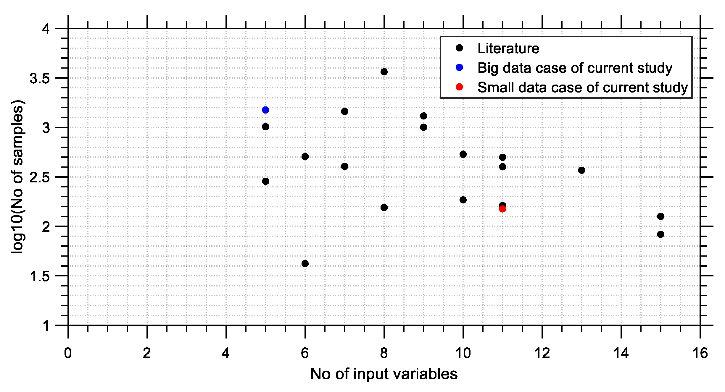
The data presented in Table 1 can be presented visually through a scattered plot, as shown in Figure 15. The horizontal axis of this plot represents the number of input parameters used for training the model, whereas the vertical axis represents the number of samples (observations). It appears that at least five input parameters are used in the various studies considered, whereas the majority of sample sizes do not exceed 1500.

The vertical axis is plotted on a logarithmic scale to enable a better visual presentation of the data. Furthermore, it is obvious that the data becomes larger as one moves towards the top left corner of the scatter plot. The opposite happens as one moves towards the bottom right corner. In the present study, it would be of interest to examine two extreme cases of experimental datasets in order to avoid loss of generality regarding the data size when investigating the performance of the proposed methodology. These two extremes correspond to the cases of maximum cases with the minimum number of input variables and minimum cases with the maximum number of input variables. For this purpose, two characteristic cases of data samples are selected, shown in red in Figure 15. These cases correspond to a “big” data case and a “small” data case, which are comprised of 1500 observations × 5 variables (denoted as 1500 × 5) and 150 observations × 11 variables (denoted as 150 × 11), respectively. Assuming that the variation of ANN predictive ability with hidden layer size will follow trends that are intermediate between the trends of the two aforementioned extreme cases, these two dataset sizes will be used in the subsequent sections. It is noted that the two selected data cases do not correspond to any cases from Table 1, but are arbitrary selections that try to simulate “big” and “small” data problems in an attempt to test the proposed methodology for these two extreme cases.

For each one of the two selected datasets as described in the previous paragraph, two types of random distributions are examined, i.e., Latin hypercube sampling (LHS) and the multivariate normal random distribution (MVNRD). The LHS contains vectors, each element of which is randomly distributed with one from equally probable (uniformly sized) intervals covering its entire range and is randomly permuted. The MVNRD contains a distribution of random vectors of correlated or non-correlated variables, where each vector element follows a univariate normal distribution. It is a generalization of the univariate normal distribution to two or more variables and is often used as a model for multivariate data. Various values of the covariance between variable pairs are examined in the two selected datasets. Ensuring the random nature of the considered distributions results in effectively shuffled data, which avoids the presence of entire minibatches of highly correlated examples, which would lead to neural networks that remember a specific order. Regarding the output variable that is contained in these datasets, for the purposes of the present study, it is defined as a symmetric function of the input variables to ensure that there is no bias not only between the labels and the features of the ANN, but also within the labels themselves. The output function has been defined as follows:

$$y_{out}=\sqrt{\sum _{i=1}^k{\left(x_i\right)}^4}.$$

(18)

where $k$ is the number of input variables in the dataset. For the various analyses that are carried out in this section, the parametric procedure outlined in Section 3.2 of the present study is used.

6.1. Case of “Big” Data

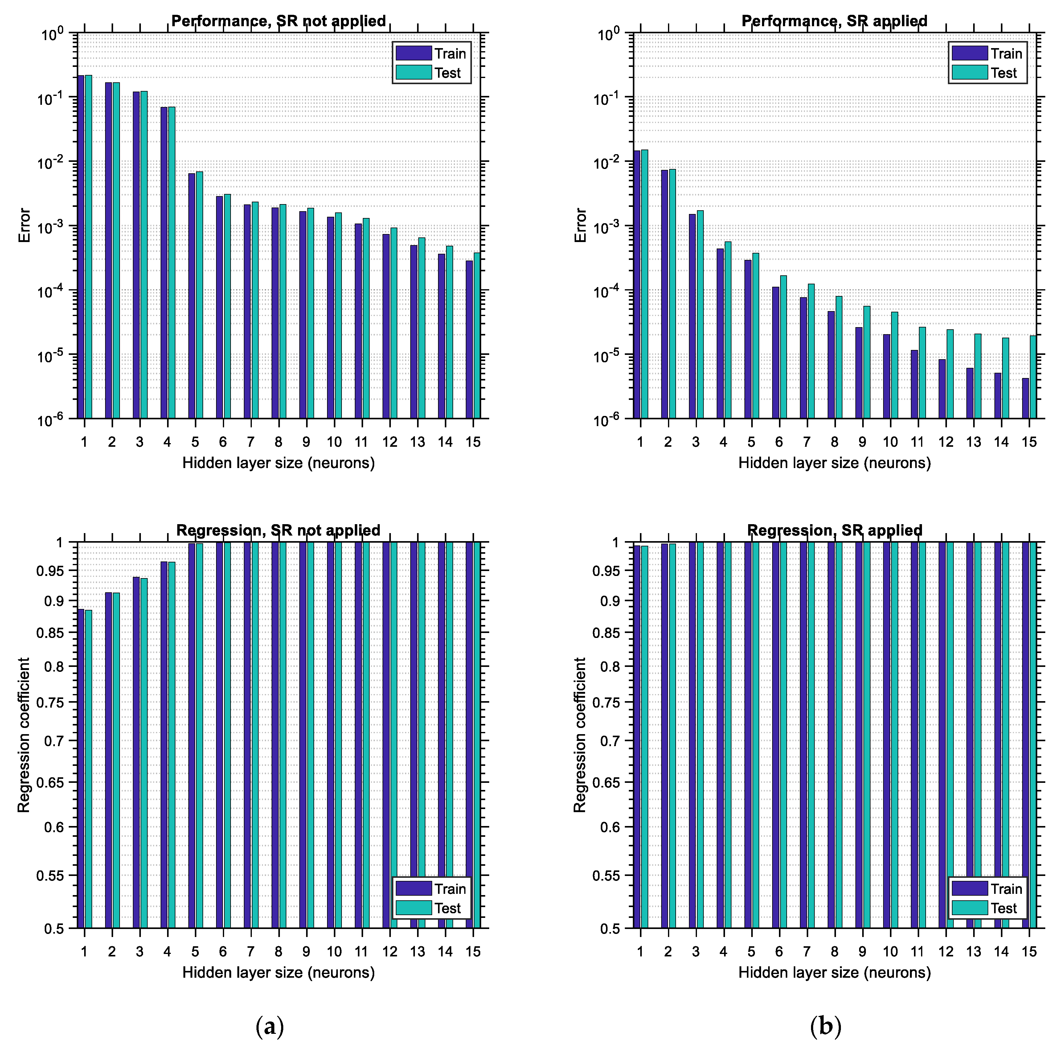
6.1.1. Latin Hypercube Sampling Distribution

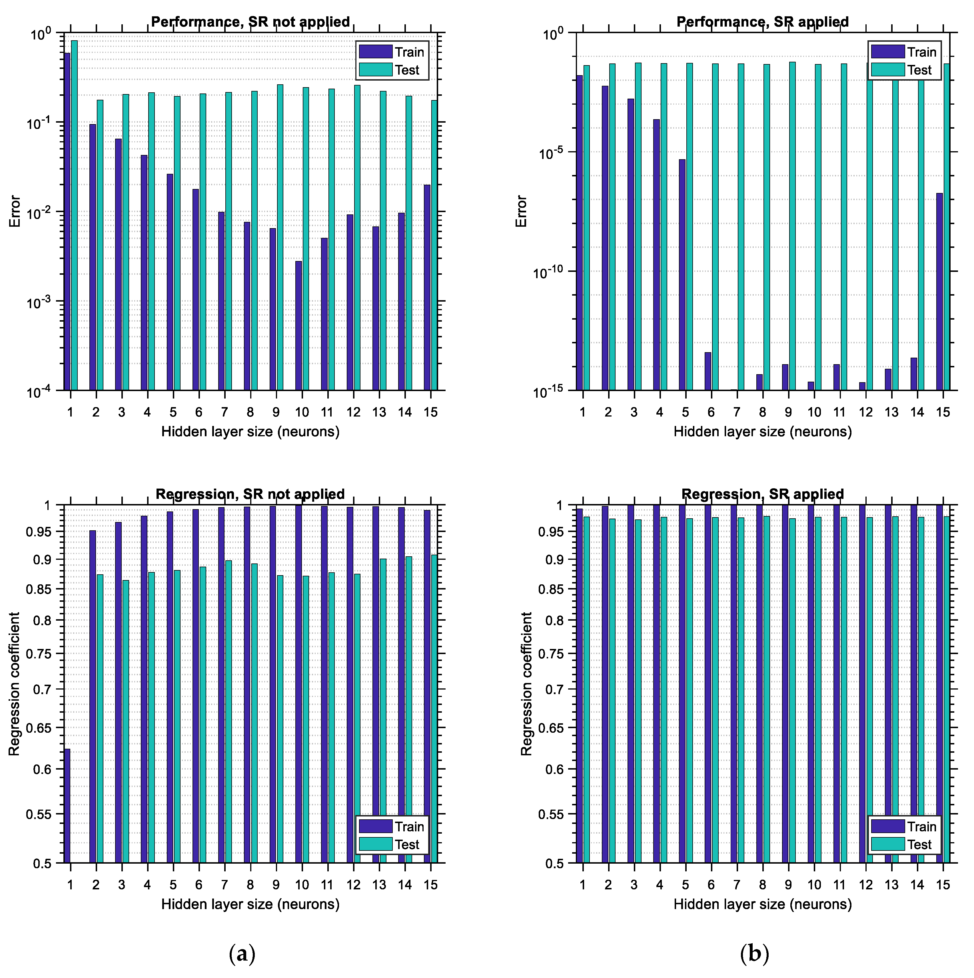
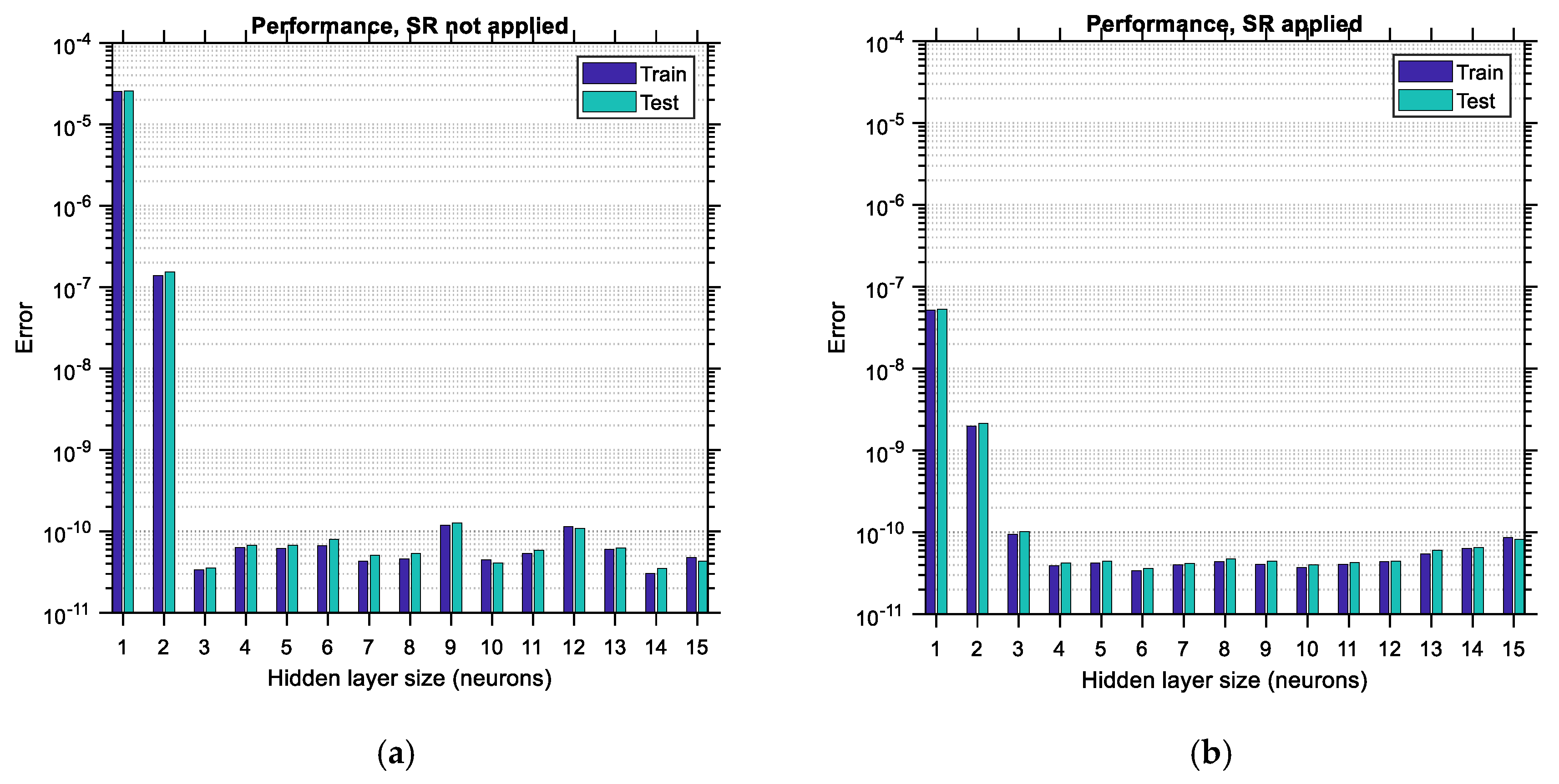
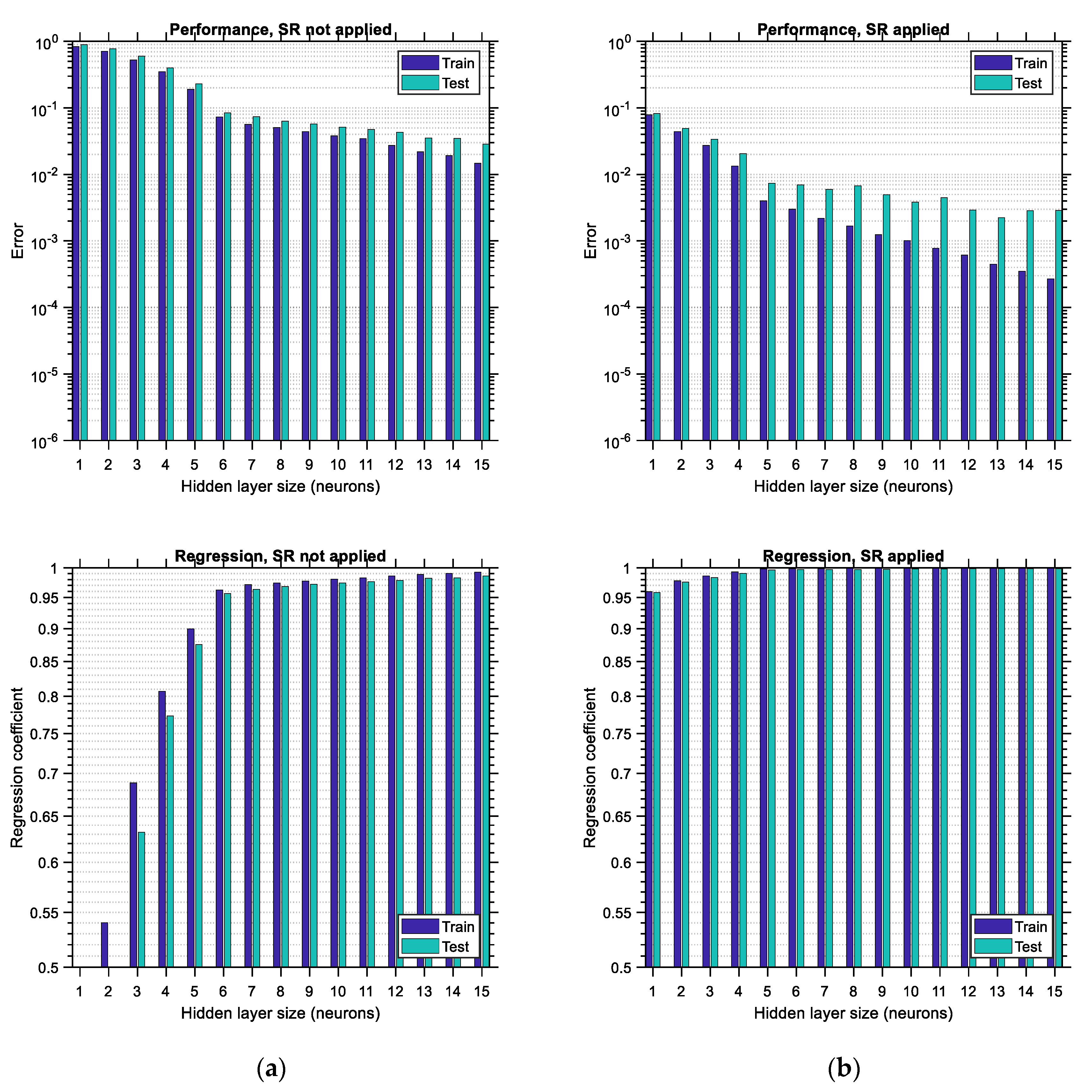
The performance error and regression coefficient between the predicted and actual output data are shown in Figure 16 for the case of data distributed according to the LHS algorithm. Each bar corresponds to one size of the hidden layer of the ANN (i.e., the number of its neurons). In the horizontal axis, the hidden layer size ranges between 1 and $n_H$, where $n_H$ is considered to be equal to 15. The upper limit of this range is arbitrarily selected so that the various trends are adequately illustrated in this study; it could be extended to higher values as well. Each bar is comprised of two sub-bars, the left of which accounts for the training error/regression and the right of which accounts for the testing error/regression. The vertical axis is set to be in logarithmic scale so that the various differences between the plots become more obvious. 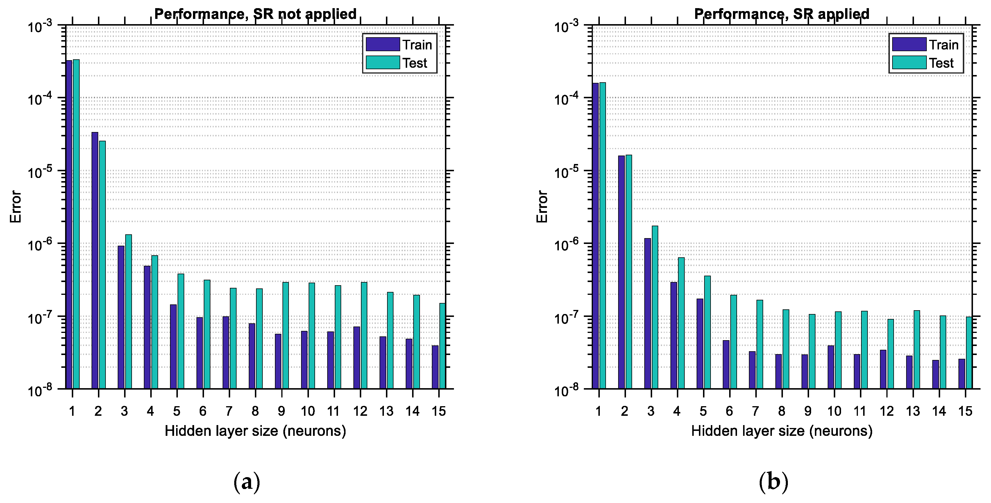By comparing the corresponding bar charts between the case where SR is not applied (i.e., BR-ANNs trained according to usual procedure) and the case where the SR procedure is applied as suggested in this study, it becomes apparent, by comparing Figure 16a,b, top and bottom, respectively, that in the latter case the testing error is reduced and also the regression of the testing data is increased. The reduction in the performance error can reach as much as 90%, whereas the improvement in the regression is of lower magnitude, especially for hidden layer sizes larger than four. This implies that the application of the SR technique leads to more accurate ANNs by roughly one order of magnitude. Furthermore, it should be observed that as the size of the hidden layer increases, the training error decreases. The same does not happen with the testing error, which, depending on whether SR is applied or not, either shows a local minimum or decreases continuously, respectively, at least for the range of the hidden layer size considered. Such local minima do not occur (and should not) for the training data since, after the hidden layer size exceeds a certain limit, overfitting occurs in the ANN involved, and as a result, the training error is supposed to continue decreasing while the testing error is supposed to start increasing. This trend is in total agreement with the trends observed in the bar charts (see Figure 16b, Figure 17b and Figure 18b, top). 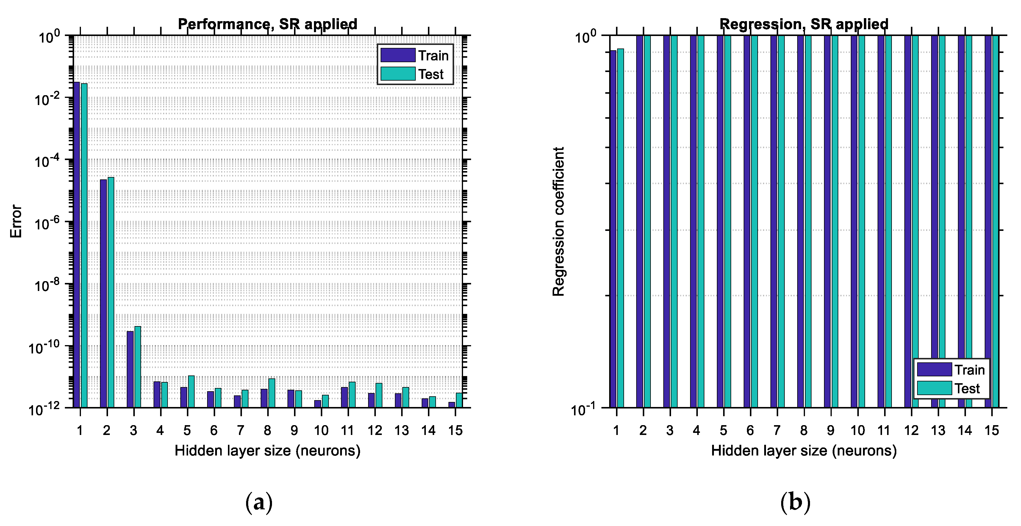The minimum testing error occurs for hidden layer sizes equal to 14 and when SR is applied for the LHS-distributed data case (as noted in Figure 16b, top). In addition to the above, it is apparent that applying the SR technique leads to higher values of regression as well, especially for lower sizes of the hidden layer.

6.1.2. Normal Random Distribution

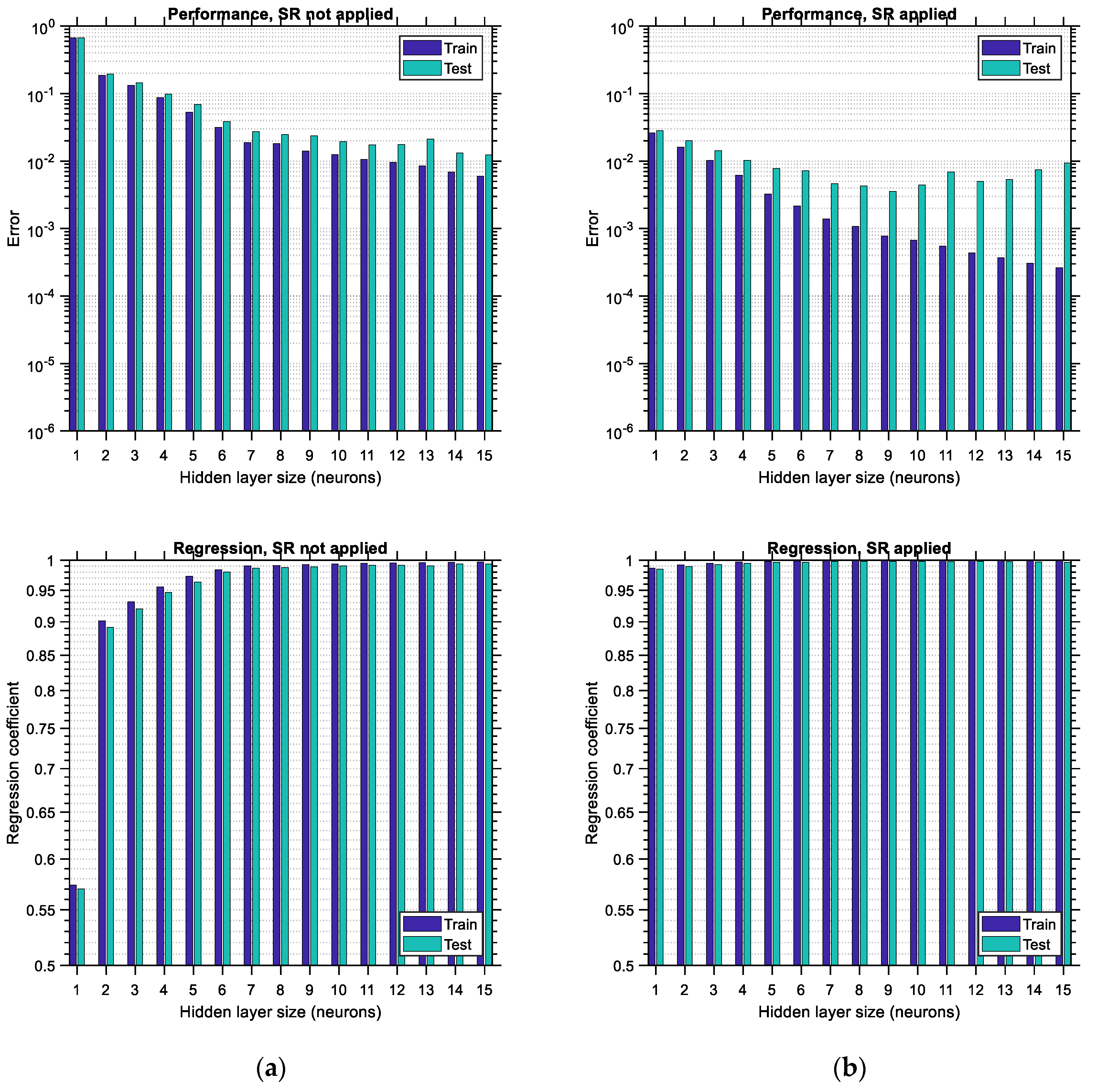
The LHS-distributed data correspond to the case of data with the highest diversity. However, how does the accuracy of the ANN vary with its hidden layer size for other data distributions? Does any correlation between the input variables have an effect on the accuracy and optimum size of the ANN? These are the questions that will be addressed in this section. In Figure 17 and Figure 18, the performance error and regression coefficient between predicted and actual output are shown for uncorrelated (zero correlation) random normally distributed data and for random normally distributed data with a relatively low correlation coefficient of 0.5, respectively. This correlation coefficient applies to all pairs between the input variables. The representations of the bar charts in Figure 17 and Figure 18 are analogous to those in Figure 16. Regarding the training data, it is observed in Figure 17 and Figure 18 that the error constantly decreases and the regression coefficient constantly increases, similar to Figure 16. Furthermore, it is seen that when SR is applied, the error in the testing data exhibits a local minimum, both for uncorrelated and correlated data distributions. For the uncorrelated data distribution, the minimum testing error occurs for a hidden layer size equal to 13 (see Figure 17b, top), whereas for the correlated data, the minimum occurs for a hidden layer size equal to 9 (see Figure 18b, top). Consequently, it seems that the required size of the hidden layer of the ANN depends on the correlation between the input data variables. This trend is expected since it is anticipated that as the correlation between the input variables increases, the patterns that have to be learned by the ANN decrease, and it is for this reason that the required ANN size (i.e., learning capacity) is lower in the latter case. In addition to these, it seems in both Figure 17 and Figure 18 that application of the SR technique leads to much lower testing errors in comparison to the case where the same ANN is trained in the usual way without applying SR. When applying SR, the regression coefficient increases as well, especially for lower hidden layer sizes.

An interesting observation comes when the minimum testing error of the uncorrelated and correlated data cases, which are 0.0021 and 0.0035, respectively, is compared (see Figure 17b and Figure 18b, top, respectively). In addition to this, the corresponding value of the minimum testing error for the LHS-distributed data is roughly 0.00002 (see Figure 16b, top), which is much lower than the error of the other two. From all the aforementioned results, it can be initially concluded that the minimum testing error when SR is applied is always lower than the testing error of ANNS, in which the SR technique is not applied for all hidden layer sizes and data distributions. However, the testing error for correlated data is higher than the testing error for uncorrelated data, which is higher than the minimum testing error for LHS-distributed data. It seems that the degree of correlation between the input variables, while acting beneficially regarding the training effort, leads to a larger prediction error. When correlation increases, the number of learning patterns decreases, the minimum prediction error increases, and the required size of the ANN decreases.

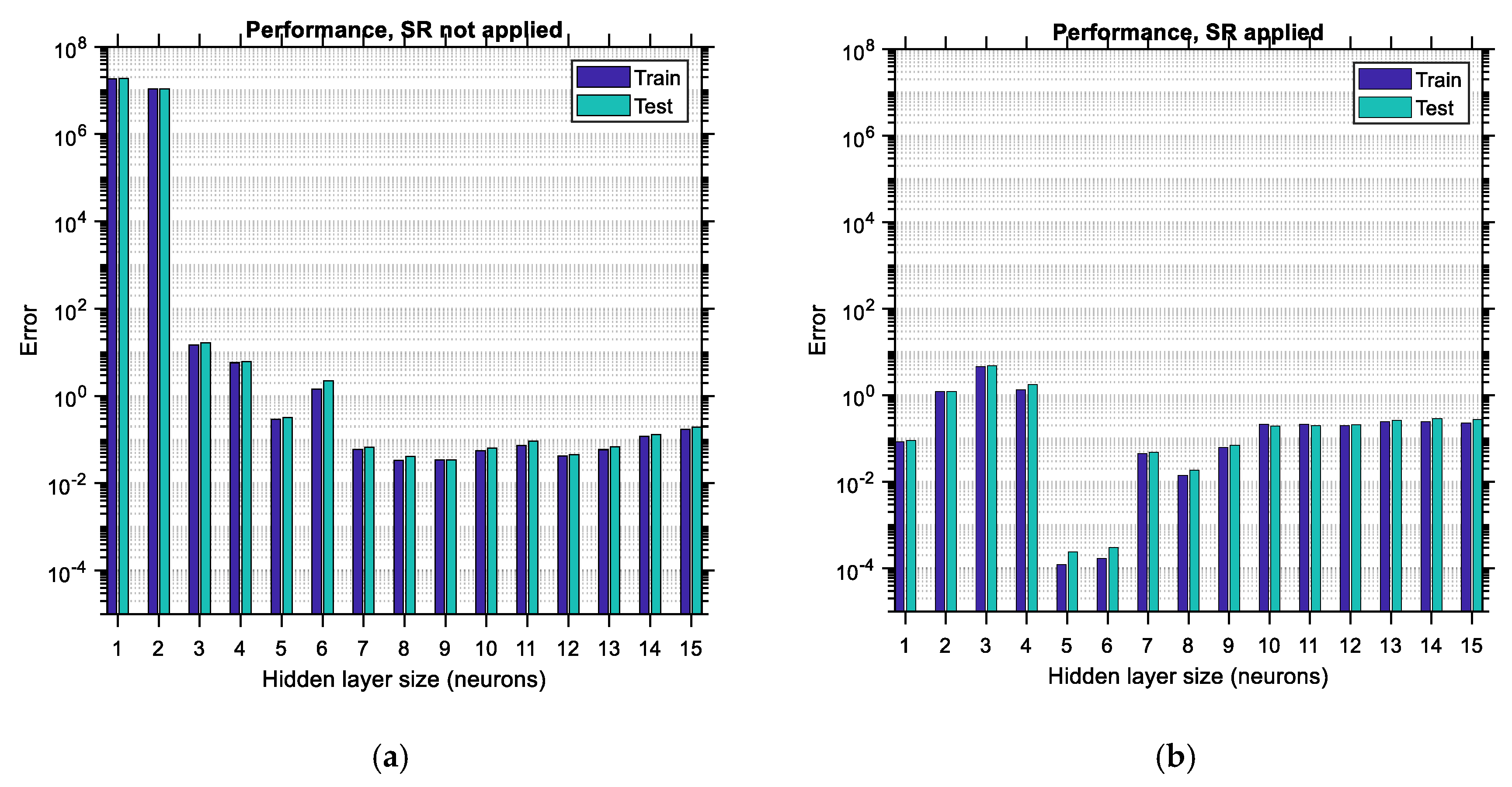
6.2. Case of “Small” Data

6.2.1. Latin Hypercube Sampling Distribution

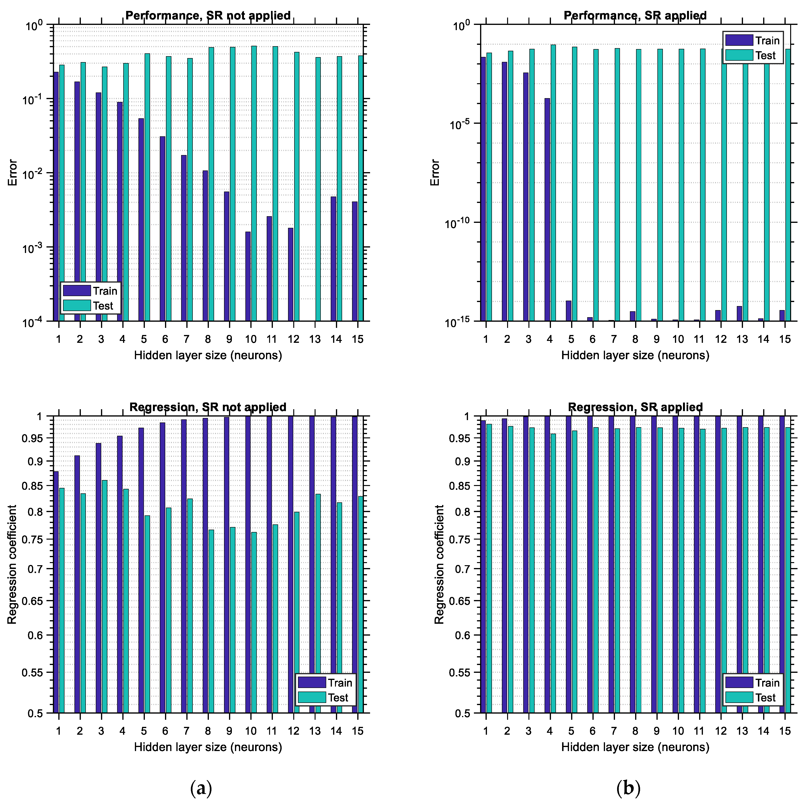
In Figure 19, the performance error and regression coefficient for LHS-distributed training and testing data are plotted for various sizes of the hidden layer of the ANN in cases of applying or not applying the SR technique. Similar to the observations made in the previous figures related to the “big” data, the performance error is substantially lower when SR is performed, and the regression coefficient is substantially higher, which leads to ANNs with higher predictive power. In addition, it is observed that application of the SR technique in ANNs trained with “small” LHS-distributed data leads to an optimum hidden layer size equal to 1, thus minimizing the computational effort required for training. However, this convenience comes with the major disadvantage of a high testing error equal to 0.035, compared to its “big” data counterpart, which is equal to 0.00002. This observation corroborates the fact that ANNs need to be trained with large data sets in order to have low prediction errors. Furthermore, it is noted that the regression of the testing data shows some irregular variations (see Figure 19a, bottom), which are stabilized in the case where SR is applied (see Figure 19b, bottom). The same happens with the performance error of the training data, which varies in a non-canonical way when SR is not applied, especially for hidden layer sizes equal to 9 or higher (see Figure 19a, top). SR seems to provide some remedy for this irregular trend, as shown at the top of Figure 19b.

6.2.2. Normal Random Distribution

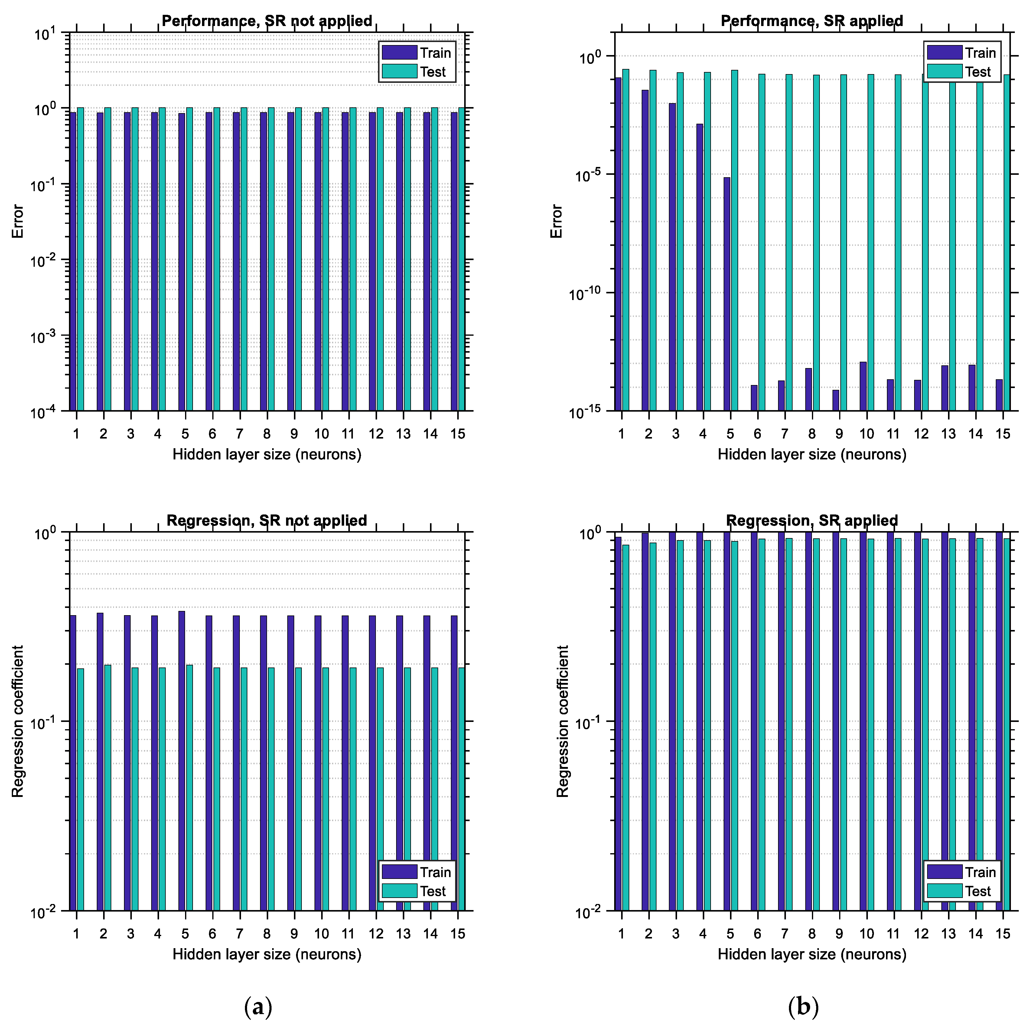
Figure 20 and Figure 21 are the “small” data counterparts of Figure 17 and Figure 18, respectively. In Figure 20a, it is observed that for “small” normal random distributed data with zero correlation, the training and testing performance error, as well as the training and testing regression coefficient, are nearly independent of the hidden layer size of the ANN. In the case where SR is applied, the training and testing errors both decrease, with the decrease in the testing error being much more subtle, as shown in Figure 20b, top. The regression coefficient slightly increases for both the training and testing data, as shown in Figure 20b, bottom. The testing error is roughly equal to 0.15 when SR is applied (see Figure 20b, top), whereas its value is roughly equal to 1 when SR is not applied (see Figure 20a, top). Things are different in the results shown in Figure 21, where the testing error is roughly 0.2 when SR is not applied (see Figure 21a, top) and roughly 0.05 when SR is applied (see Figure 21b, top). The aforementioned observations suggest that any correlation between input variables in “small” data cases may lead to reduced performance error, contrary to the “big” data case. It remains to be studied if this is a general trend and the factors on which it depends. Furthermore, it is seen that for the correlated “small” random normally distributed data case and in the case that SR is not applied, the training error does not vary regularly, especially for hidden layer sizes of 9 or higher (see Figure 21a, top). The most important observation regarding the “small” data case is that the application of SR prior to training an ANN works beneficially regarding both the performance error and the regression coefficient, in a way similar to the “big” data case.

7. Discussion

In

Table 2. Results of the proposed SR-ANN method for fixed and optimum ANN architectures, regarding the benchmark problems presented in Section 5.1, Section 5.2 and Section 5.3.

Approximated Function	Fixed H (According to [29])	Max. Error for Fixed H [29]	Max. Error for Fixed H (SR-ANN)	Optimum H (SR-ANN)	Max. Error for Optimum H (SR-ANN)	Accuracy Gain for Fixed H
Cosine	2	5.5%	0.19%	14	0.05%	28.95×
Gamma	20	0.65%	0.1%	12	0.4%	6.5×
Upper tail integral of the Gauss distribution function	20	0.3%	0.1%	6	0.0025%	3×

, the three cases of function approximation using ANNs described in Section 5.1, Section 5.2 and Section 5.3 of this study are presented in concise form for a better understanding of the benefits of the proposed SR-ANN method in terms of accuracy. Two cases of the architecture of the ANNs involved (i.e., size of hidden layer, denoted as H in Table 2) are considered in the results presented in this table, i.e., a fixed architecture as assumed in [29] and an optimum architecture as found by the parametric analysis proposed in Section 3.2 of the present study. The maximum errors (a) observed in reference [29], (b) found by the proposed SR-ANN algorithm for fixed H, and (c) found by the proposed SR-ANN algorithm for optimum H are presented in the table. In addition, in the last column of this table, the gain in accuracy is presented (i.e., the ratio of the maximum error for fixed H according to [29] to the maximum error for fixed H according to SR-ANN). 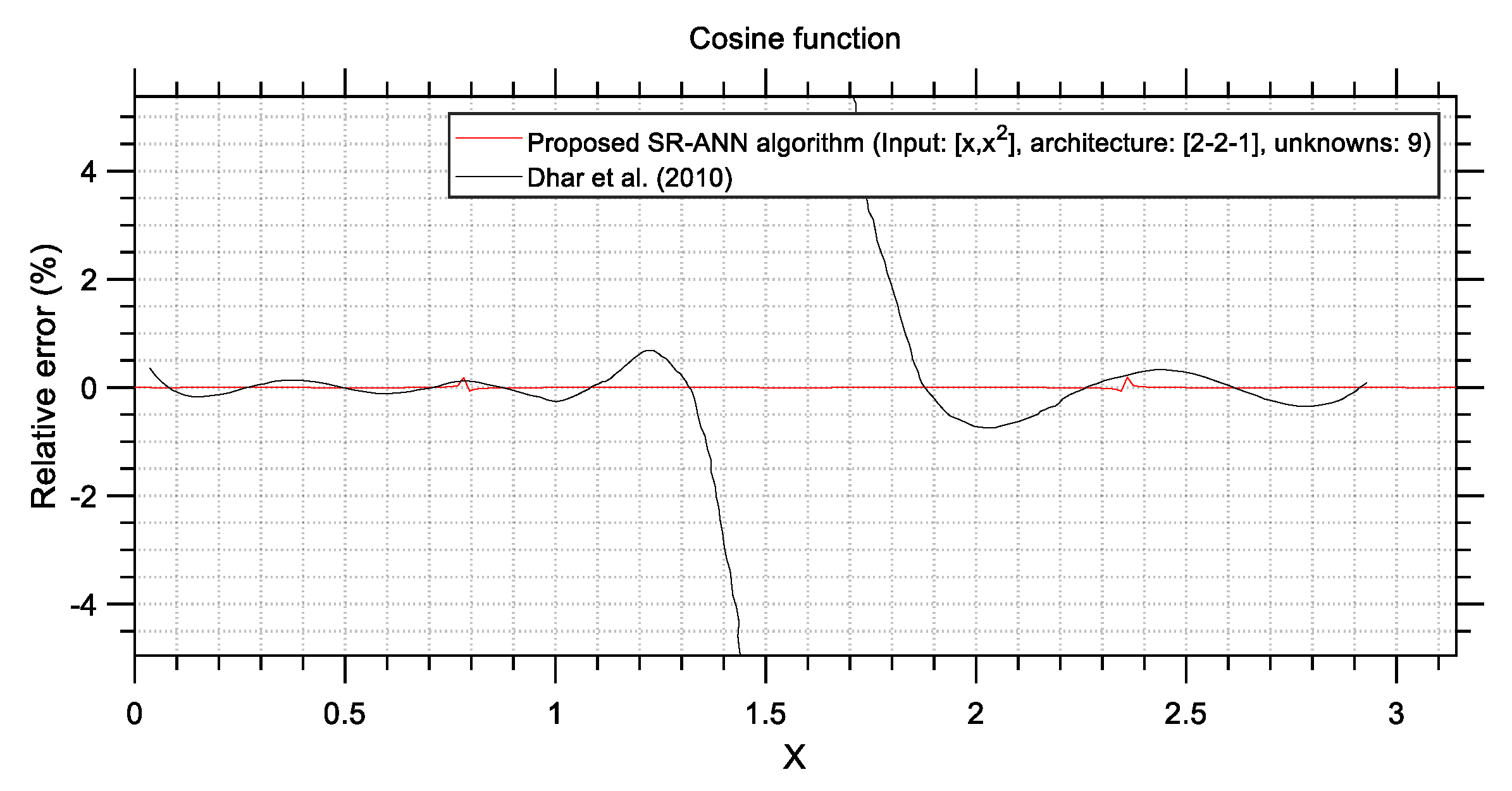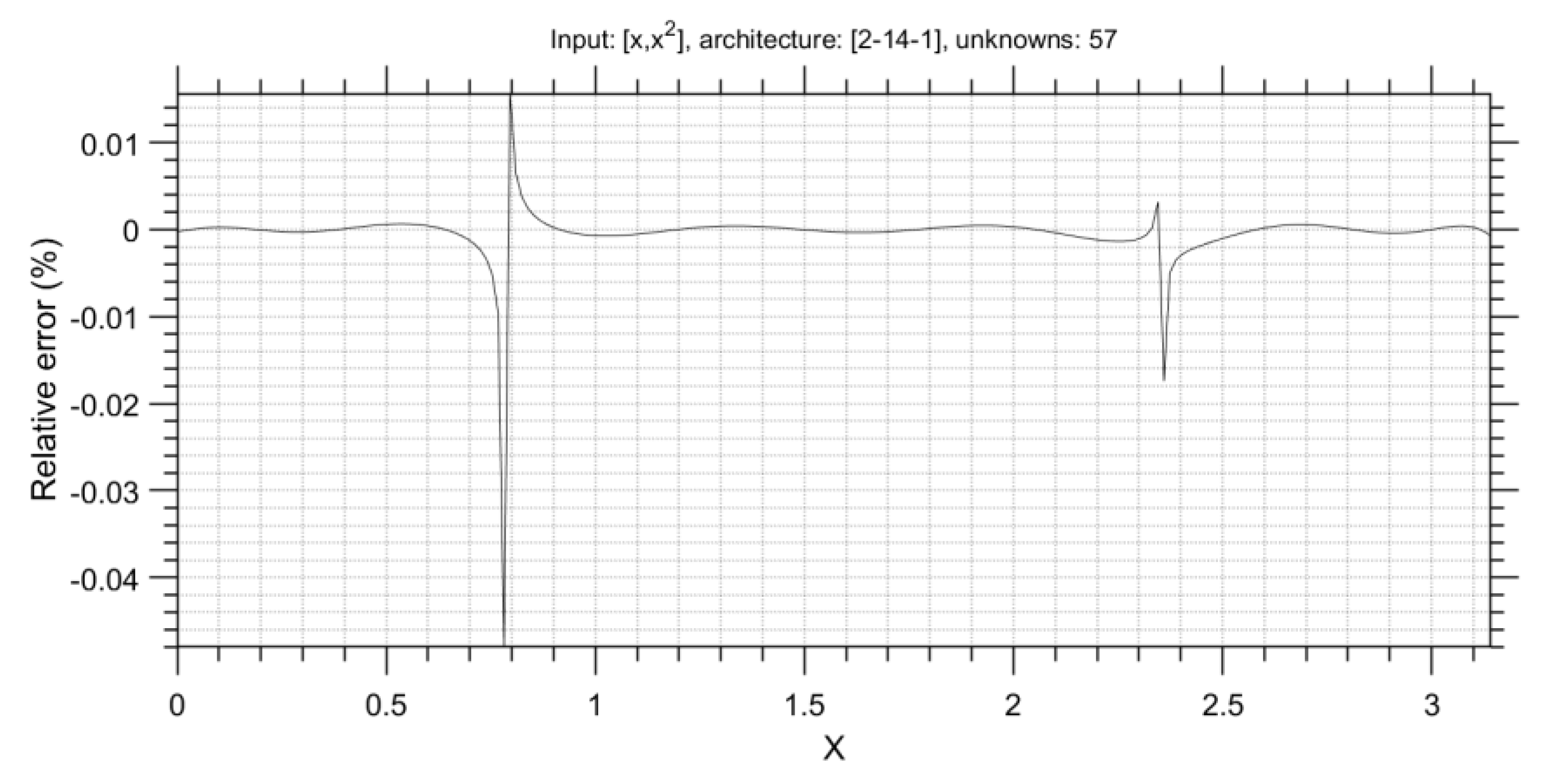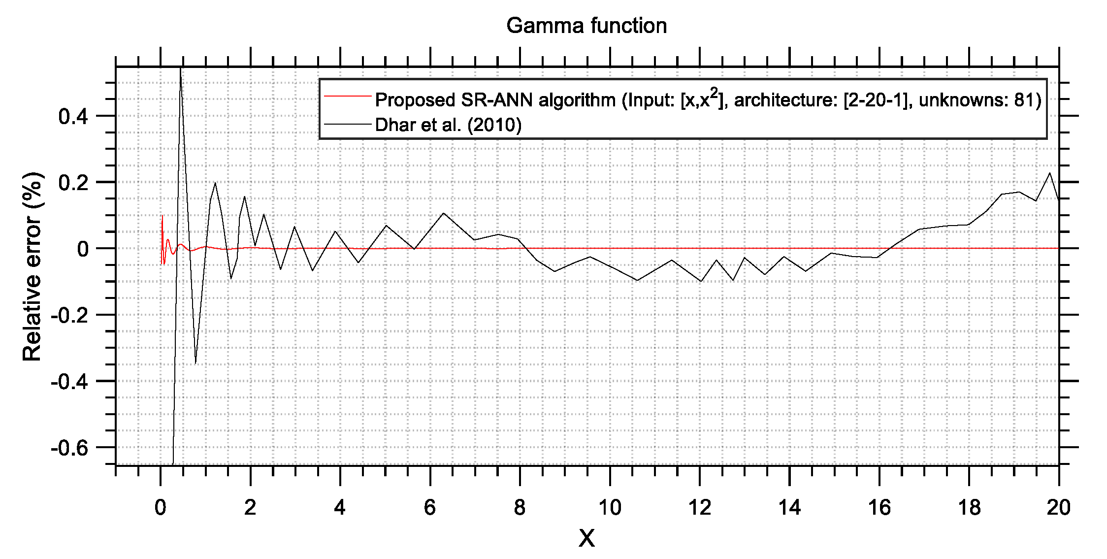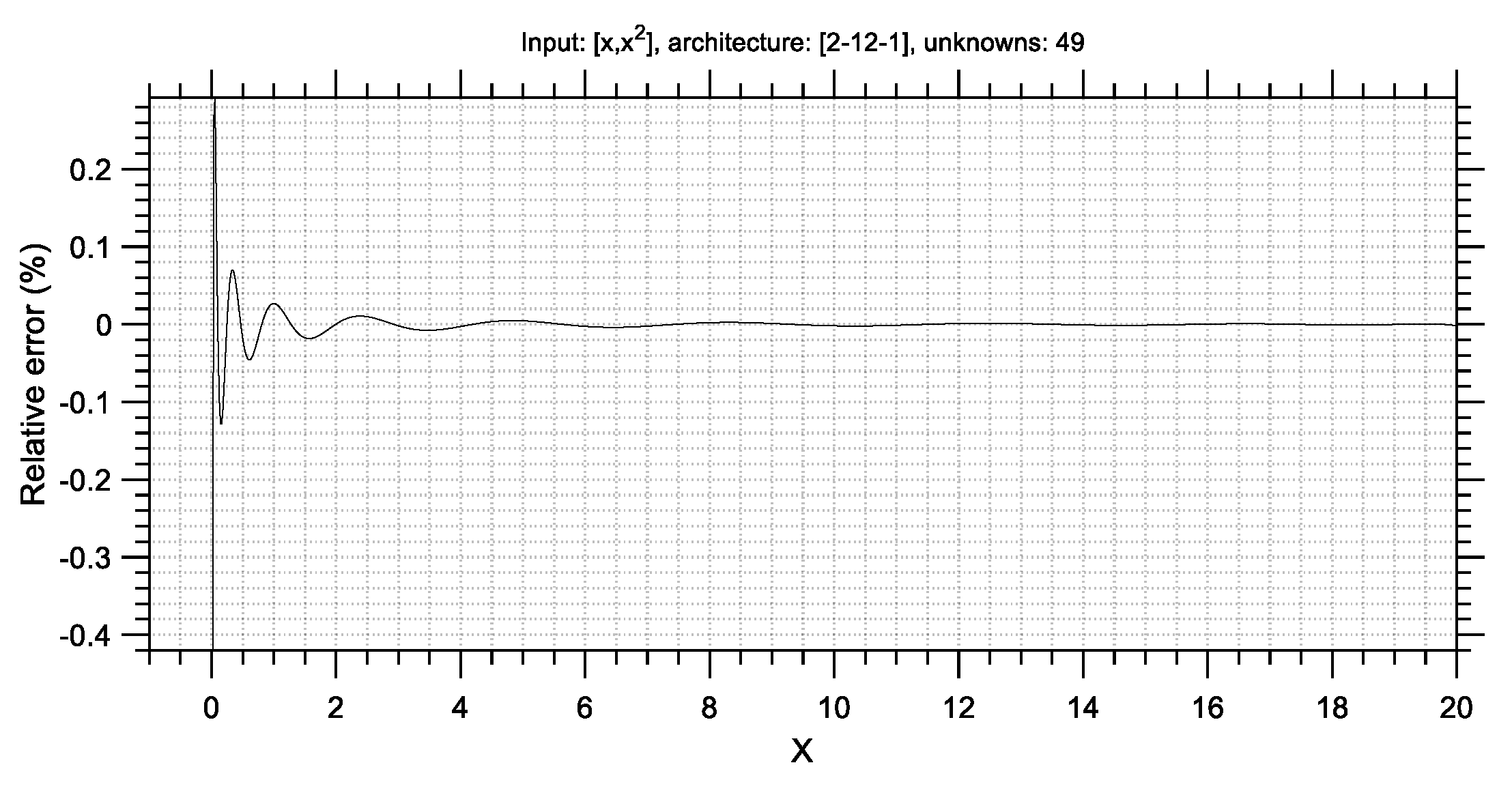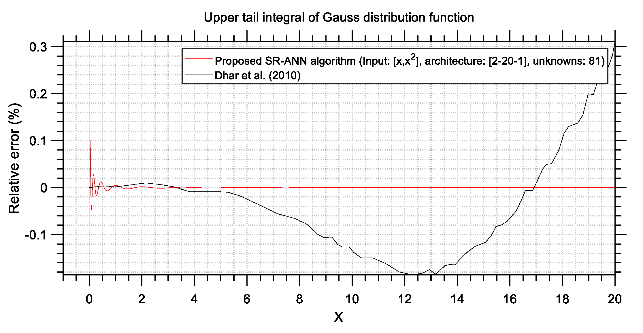From the results of Table 2, it is apparent that the proposed SR-ANN algorithm yields ANNs that are capable of as much as 28.95 times more accurate predictions compared to ANNs trained with conventional methods, while it seems that increasing the size of an ANN does not always lead to better accuracy.

In

Table 3. Results of ANNs trained with the BR algorithm, with and without application of SR, for multivariate problems with various data sizes and distributions considered in Section 6.

Distribution Type	Correlation	Hidden Layer Size (Minimum Performance Error, SR Applied)	Unknowns (SR Not Applied)	Prediction Error (SR Not Applied)	Unknowns (SR Applied)	Prediction Error (SR Applied)	Accuracy Gain
		(a)	(b)	(c)	(d)	(e)	(f)
Big data (1500 observations × 5 variables)
LHS	-	14	99	0.0004786	309	0.00001793	26.69×
MVNRD	0	13	92	0.0351	196	0.0022	15.95×
MVNRD	0.5	9	64	0.0238	199	0.0035	6.8×
Small data (150 observations × 11 variables)
LHS	-	1	14	0.2839	34	0.0362	7.84×
MVNRD	0	14	183	1.0083	407	0.1521	6.63×
MVNRD	0.5	1	14	0.809	34	0.0411	19.68×

, a review of the various results obtained in Section 6 is provided for a better view and easier comparisons. There are two main parts to this table, referring to the big data case and the small data case. For each one of the two cases, the distribution type and its correlation value are shown in the left column, whereas in the top row, the following are provided: (a) the size of the hidden layer of the ANN for which minimum testing error was observed; (b) the number of unknowns (weights and biases) in the case of ANN with hidden layer size that of (a) and the SR technique not applied; (c) the prediction error in case (b); (d) the number of unknowns (weights and biases) in the case of ANN with hidden layer size that of (a) and the SR technique applied; (e) the prediction error in case (d); and (f) the gain in accuracy due to application of SR technique (i.e., how many times lower the error in column (e) is compared to column (c). It is obvious that there is a gain in accuracy higher than 6 in all cases of data size and data distributions. This justifies the benefits that result from applying the proposed technique during ANN development.

8. Conclusions and Future Work

In this study, a new methodology, the step regression-artificial neural network (SR-ANN) algorithm, is proposed for increasing the prediction accuracy of feedforward ANNs while reducing the size of the hidden layer. A simplified classification problem has been examined first, in which it is proved that SR can result in an ANN with fewer parameters (weights and biases) than its ordinary counterpart, even without any hidden layer, while still (the ANN) being able to perform nonlinear classification. From this observation, it became apparent that the application of the SR algorithm may reduce the required computational effort required to train an ANN. In the next sections of this study, this scenario has been investigated for some benchmark and advanced problems, where the beneficial effect of the SR technique has been confirmed for all cases examined.

It has been found that the proposed SR-ANN algorithm increases the prediction accuracy of ANNs and the regression coefficient between their predicted and actual output. The workflow for its application is provided, and its benefits are shown through verification and investigative analyses. In addition, it is shown that the required number of hidden neurons in an ANN that minimizes the testing error is higher in the case of the LHS distribution dataset compared to the normal random distribution dataset, due to the maximized number of learning patterns included in the former. This provides strong evidence that the optimum size of an ANN that is used to learn some training data depends, apart from other factors, on the distribution and diversity of the data as well. Furthermore, it is concluded that application of SR prior to training is beneficial for ANNs in two ways: (i) it substantially decreases the performance error for the various hidden layer sizes, and (ii) it generally decreases the optimum hidden layer size, thus reducing the required computational effort for training. Moreover, it has become apparent that the addition of nonlinear terms in the input layer, in combination with the nonlinearity stemming from the transfer functions of an ANN, increases the degree of its nonlinearity, thus making it more robust and accurate in difficult situations. By adding nonlinear terms to the input data that maximize regression, the SR procedure helps the ANN be more accurate by adding some kind of “knowledge” to it. The application of the SR-ANN algorithm determines the terms in the input layer in an automated way and thus minimizes human intervention and subjectivity in the training process. Finally, the dual role of SR, which can be perceived either as a training data augmentation technique or as an automatic ANN configuration tool (regarding its input layer), has been postulated, and its deep implications regarding the design of ANNs have been stated. It has also been shown in Section 4.4 that the SR technique and ANNs are in various ways complementary to each other, and therefore the proposed SR-ANN method is not a simple modification of existing methods, but it exploits the deeper traits of the two aforementioned methods to effectively incorporate them into an integrated method.

Some ideas for future work include, but are not limited to, the following:

(1)

The (quadratic) SR procedure suggested in this study can be generalized in various ways, e.g., consideration of exponents higher than 2 and/or inclusion of inverse terms (i.e., negative exponents) of the initial variables, thus effectively forming ratios between them as well. It is almost certain that this will lead to even more robust regression ANNs with high prediction accuracy, and they will also be able to handle more complex problems.

(2)

SR can be applied not only in the input layer, as is performed in this study, but also in the intermediate hidden layer(s) of the ANNs as well. This possibility may be explored in a future study by the author.

(3)

It is of interest to apply the SR algorithm to deeper ANNs and see the variation in the number of neurons in each hidden layer and, most importantly, how the training effort is varied when applying the SR procedure.

(4)

The influence of the number of nonlinear terms added through the SR procedure in the input variables of a training dataset on the prediction accuracy of the ANN could be investigated. There may be an equilibrium point between SR and ANN training that takes advantage of both tools in the best way, minimizing the overall computational effort.