Article

Controller Design for Air Conditioner of a Vehicle with Three Control Inputs Using Model Predictive Control

Department of Mechanical, Automotive & Materials Engineering, University of Windsor, 401 Sunset Ave., Windsor, ON N9B 3P4, Canada
*
Author to whom correspondence should be addressed.
Modelling 2024, 5(1), 117-152; https://doi.org/10.3390/modelling5010008
Submission received: 21 November 2023 / Revised: 20 December 2023 / Accepted: 27 December 2023 / Published: 3 January 2024

Abstract

:
Fuel consumption optimization is a critical field of research within the automotive industry to meet consumer expectations and regulatory requirements. A reduction in fuel consumption can be achieved by reducing the energy consumed by the vehicle. Several subsystems contribute to the overall energy consumption of the vehicle, including the air conditioning (A/C) system. The loads within the A/C system are mainly contributed by the compressor, condenser fan, and underhood aerodynamic drag, which are the components targeted for overall vehicle energy use reduction in this paper. This paper explores a new avenue for A/C system control by considering the power consumption due to vehicle drag (regulated by the condenser fan and active grille shutters (AGS)) to reduce the energy consumption of the A/C system and improve the overall vehicle fuel economy. The control approach used in this paper is model predictive control (MPC). The controller is designed in Simulink, where the compressor clutch signal, condenser fan speed, and AGS open-fraction are inputs. The controller is connected to a high-fidelity vehicle model in Gamma Technologies (GT)-Suite (which is treated as the real physical vehicle) to form a software-in-the-loop simulation environment, where the controller sends actuator inputs to GT-Suite and the vehicle response is sent back to the controller in Simulink. Quadratic programming is used to solve the MPC optimization problem and determine the optimal input trajectory at each time step. The results indicate that using MPC to control the compressor clutch, condenser fan, and AGS can provide a 37.6% reduction in the overall A/C system energy consumption and a 32.7% reduction in the error for the air temperature reference tracking compared to the conventional baseline proportional integral derivative control present in the GT-Suite model.

1. Introduction

The most effective method for A/C system control has been continuously evolving throughout the years as the state of the art for control design has also continued to evolve. Early implementations of controllers on A/C systems include on/off, proportional integral derivative (PID), and sliding-mode controllers. Høgh and Nielsen [1] presented a new and innovative control strategy that used a compressor and an electronic expansion valve for better control of the superheat level. The system efficiency was also analyzed to find the optimal superheat setpoint, which could reduce energy consumption. The refrigerant system was modeled to allow for model-based feedback and feedforward, which improved control of the superheat level. Koo et al. [2] discussed the use of a proportional–integral (PI)-controlled cascade structure to control the relative filling and evaporation pressure of a target system. They also introduced the super-twisting-algorithm-based 2-sliding mode controller (SMC) design for the target system. The 2-SMC design was found to be more effective than the classical first-order sliding mode controller (1-SMC) in handling plant parameter uncertainty. Liu et al. have worked on a survey [3] where they provided a comprehensive overview of different automatic control techniques that had been applied in A/C systems. The authors described the characteristics of A/C systems and discussed the variables that should be controlled. They used classification of the control approaches to explain the main features of these strategies used in A/C systems. Their paper clearly showed that, with the improvement in people’s living standards and the emergence of global environmental and energy problems, there were increasing requirements for more advanced A/C control strategies. The authors summarized studies of control methods presented in the paper, and analyzed the development and new trends of A/C control approaches. Additionally, the paper discussed studies of PID control applied in A/C systems, including more advanced PID control methods to improve control system performance and to make full use of PID control advantages in the multi-input–multi-output (MIMO) A/C system control, and simplify the design and operation procedure of the control strategies. The above-mentioned controller designs are typically applied to the compressor to maintain the cabin at a specific temperature. These controllers are simple to design but most do not attempt to reduce the energy consumption of the system. Cvok et al. [4] proposed a method to optimize and control an electric vehicle heating, ventilation, and air conditioning (HVAC) system for better efficiency and thermal comfort. The authors used dynamic programming to find optimal control actions based on a simplified cabin model and static HVAC maps. They also designed a hierarchical control system that used an instantaneous optimization-based allocation algorithm and a superimposed cabin temperature controller. They verified their method by simulation for a cool-down scenario and compared it with the dynamic programming benchmark. They showed that their method could approach the benchmark by tuning the controller bandwidth and the allocation cost function. Kim et al. [5] presented the development of a mathematical dynamic model and observer-based set point control of a vapor compression cycle (VCC) system. The mean void fraction and moving boundary control volumes in a heat exchanger (HEX) were used for a lumped parameter model of an air conditioning system. A MIMO dynamic model of the VCC was presented in a nonlinear state space representation (SSR) and was reformulated into a linearized regular form for control design. A modified observer-based controller with SMC was introduced to attenuate the effects of observing approximation errors and external disturbances. The proposed control methodology ensured uniformly ultimately bounded tracking results of the desired low pressure and suction superheat. A simulation of controlling the VCC illustrated the effectiveness and performance in the presence of disturbances. Xie et al. [6] proposed an intelligent air conditioning system control strategy that can learn passengers’ thermal comfort preferences. The proposed control algorithm directly and automatically decreased the cabin temperature to the passengers’ preferred temperature without any manual adjustment.
More recent developments in sliding-mode controller applications show potential for energy savings related to the operation of the compressor and fans. However, these control methods still lack any consideration of vehicle drag and AGS control. For example, Huang et al. [7] presented an energy-saving controller for automotive air-conditioning/refrigeration (A/C-R) systems. The proposed controller consisted of two different time-scale layers. The outer or the slow time-scale layer, called a setpoint optimizer, is used to find the set points related to energy efficiency by using the steady-state model, whereas the inner or the fast time-scale layer is used to track the obtained set points. In the inner loop, thanks to its robustness, an SMC was utilized to track the set point of the cargo temperature.
In recent years, model predictive control applications for A/C systems have seen more research interest in academia. MPC lends itself well to A/C system control because it can directly consider constraints on inputs, states, and outputs in the control problem formulation. Liberati et al. [8] address the emerging challenge of managing smart microgrids for electric vehicle charging and various user loads while incorporating renewable energy sources and storage. Their work emphasizes the importance of advanced power systems and building automation control for real-world applications. The article introduces an economic model predictive control method that optimizes electric and heating resources in smart buildings, achieving nearly zero energy consumption and seamless participation in demand response programs. Simulation results, based on an Italian case study, showcase the approach’s effectiveness in managing electric and thermal flexibility within a building. In a review by Borreggine et al. [9] on the state-of-the-art issues and solutions for MPC in power electronics, the authors reviewed the MPC techniques for power electronics and electrical drives, with a focus on finite control set MPC and explicit MPC. The paper discussed the advantages and drawbacks of both methods, such as flexibility, performance, computation effort, and steady-state error. The paper also presented several applications of MPC for different types of converters, loads, and powertrain configurations. The paper highlighted the potential of MPC for powertrain control, especially for hybrid and electric vehicles.
More recently, MPC applications have been applied to automotive A/C systems. Most of the current literature on automotive A/C system control focuses on minimizing the compressor power consumption and the tracking error of the discharge air (cooling requirement) in electric vehicles (EVs), as discussed in a review by Huang et al. [10]. Wang et al. [11] proposed a nonlinear MPC control for EVs to minimize evaporator blower power consumption but did not consider the AGS in the analysis. Pereira et al. [12] proposed an energy management system (EMS) for a fuel cell (FC) hybrid electric vehicle based on nonlinear model predictive control (NMPC) and a recurrent neural network (RNN). The NMPC allowed the formulation of control objectives not allowed by a linear MPC, such as maximum efficiency point tracking of the FC, while the RNN accurately predicted the FC nonlinear dynamics. The EMS was implemented on a low-cost development board and tested in real time on a hardware-in-the-loop test bench equipped with a real 3-kW FC stack. The experimental results demonstrated that the NMPC EMS was able to meet the vehicle’s energy demand and operate the FC in its most efficient region. A comparative study was performed between the proposed NMPC, a linear MPC, and hysteresis band control. The results of this comparative study demonstrated that the NMPC provided better fuel economy and could reduce FC degradation. Xie et al. [13] presented an Intelligent Model Predictive Control (IMPC) strategy for the A/C–cabin coupled system that includes the influences of vehicle speed and external environment on the heat exchange with the cabin. The IMPC strategy integrates the vehicle speed previewer and the self-adaptor for passengers’ thermal comfort. The IMPC has a more dynamic response of compressor speed to the car speed change and can automatically adjust cabin temperature, making it satisfy the thermal preference of the passenger with little control error of cabin temperature. The IMPC strategy saves more energy than other control strategies researched in their paper. Glos et al. [14] presented an application of NMPC algorithms for energy-efficient control of cabin temperature and air quality in fully electric vehicles (FEVs). The authors developed simplified dynamic models of the FEV cabin and HVAC system and formulated an optimal control problem that minimized power consumption while satisfying the user’s comfort and safety requirements. The NMPC algorithms were implemented on a microcontroller and tested in a Processor in the Loop simulation. The paper showed that the NMPC approach could reduce the heat losses through ventilation and improve the range of the FEV. The paper also discussed the challenges and limitations of the NMPC implementation, such as computational complexity, state estimation, and actuator constraints. Kibalama et al. [15] presented an energy management strategy for the air conditioning system of an electrified vehicle, based on MPC. The authors used a nonlinear model of the vapor compression refrigeration system and formulated a constrained optimal control problem to minimize the energy consumption while tracking a desired evaporator pressure. They proposed a novel implementation method that reduced the computation time by approximating the value function from a global optimal solution obtained by dynamic programming (DP). They showed that their MPC approach achieved near-optimal performance on different drive cycles and thermal load requirements, and validated it on real-time hardware. The paper did not address the robustness of the controller to uncertainties or disturbances, or the extension to other thermal management systems.
A recent study by Göltz and Sawodny [16] investigated tracking performance and energy consumption of the A/C system using various control schemes, including MPC. However, this work mainly focuses on battery thermal management for battery electric vehicles (BEVs). Additionally, opening the AGS increases the cooling effort supported by the front-end airflow, allowing other components, such as the compressor, to reduce their working load and still satisfy the cooling requirements of the vehicle, as shown in a study by El-Sharkawy et al. [17]. This AGS airflow cooling comes at a cost. Shigarkanthi et al. [18] demonstrated that, as the AGS is opened, the drag force of the underhood vehicle airflow increases due to an increase in drag coefficient, concluding that the AGS has an impact on the fuel economy and power consumption of the vehicle. By controlling the condenser fan and AGS along with the compressor, it is expected that the energy used by the system can be further reduced but the cost of increased underhood drag must be considered.
Chen et al. [19] discuss the significance of real-time optimal control in improving the energy efficiency of cabin climate control systems in EVs. They introduced a novel linear-time-varying (LTV) MPC approach, which simplifies the optimization process and conducts a comprehensive parametric study to identify robust weighting factors. Comparative analysis reveals that the LTV-MPC outperforms rule-based and nonlinear economic MPC (NEMPC) controllers, achieving faster temperature regulation with significantly lower energy consumption while maintaining comparable computational efficiency.
Coppola et al. [20] focused on improving energy performance in platoons of autonomous connected vehicles. Their study presents an innovative Eco-Driving Control Architecture that utilizes NMPC for optimizing energy consumption while maintaining precise leader tracking. Analytical proofs of exponential stability and robust stability conditions are provided, demonstrating the effectiveness of the approach in various operational scenarios and parameter uncertainties within a Mixed Traffic Simulator (MiTraS) co-simulation platform. The results validate the architecture’s ability to ensure eco-driving behavior for the entire vehicle platoon.
He et al. [21] introduced a stochastic model predictive controller (SMPC) for enhancing the energy efficiency of EV air conditioning systems. It employs a Markov-chain-based velocity predictor to anticipate future disturbances, and systematically quantifies the sensitivity of the electrified AC system to solar radiation, ambient temperature, and relative air flow speed. Comparative analysis with a rule-based controller and dynamic programming benchmark reveals that SMPC improves AC energy economy by 12%, reduces cabin temperature variation by over 50.4%, and enhances overall cabin comfort.
Huang et al. [22] presented a robust model predictive controller for enhancing temperature performance and reducing energy consumption in automotive air-conditioning/refrigeration (A/C-R) systems with three-speed and continuously-varying compressors. It includes a discrete MPC with a carefully chosen terminal weight for robustness under various conditions. The study also presents hybrid controllers that combine on/off control and discrete MPC, as well as a continuous MPC for systems with variable components, demonstrating energy savings of up to 23% compared to conventional on/off controllers in both experimental and simulation results.
Based on the reviewed literature, the existing work on the application of MPC in A/C for commercial vehicles does not consider the impact of the AGS actuator nor the power consumption due to underhood aerodynamic drag [16]. Additionally, some studies have not considered all possible control inputs in the overall design, such as missing AGS [11]. Furthermore, most studies, especially in recent years, focus on EVs as energy consumption and management has a much greater role in such vehicles [12,13,14,15]. This has left fossil-fueled energy management and A/C energy efficiency on the back burner in recent years. Additionally, the applications of nonlinear controllers, although more advanced and capable, require more computation and consideration compared to simpler alternatives.
Contribution: To the best of the authors’ knowledge [23,24], the consideration of AGS control to reduce the overall vehicle power consumption and regulate the underhood airflow for cabin cooling has not been considered in the literature. Therefore, the work in this paper addresses a gap for non-electric vehicles, and additional control inputs and modeling enhancements not currently addressed in the literature. The starting point for this study is the modeling and control work by Zhang [25], where various control approaches were attempted for an internal-combustion-powered vehicle, with both the condenser fan and compressor clutch as actuators. Zhang [25] found that none of the approaches attempted was satisfactory and recommended MPC be attempted. In this paper, we apply MPC for the same vehicle, introduce the AGS as a new actuator into the control problem, and consider the additional underhood drag power consumption for the A/C system.
Several linear approximation MPCs have been formulated in the past, with the most popular being adaptive, as showcased by Dhar and Bhasin [26], and gain-scheduled model predictive controllers, as showcased by Hu et al. [27] for a commercial vehicle air brake system. These controller types will be discussed in more detail in Section 2.1. However, adaptive MPC is more promising for the application in this study due to its effectiveness for control designs where the structure of the optimization problem (number of states and constraints) remains the same across different operating points. Further discussions and rationales for the choice of adaptive MPC in this study are provided in Section 2.1. To address the identified gap in the literature and extend the work by Zhang [25] based on the system modeling improvements for the A/C system by the authors in [28], this paper has two main objectives:
  • Objective 1. In addition to controlling the compressor clutch only, determine the improvement in A/C system energy use and air-to-cabin reference temperature tracking that can be achieved by switching from PID (benchmark) to MPC.
  • Objective 2. Identify what further improvement, if any, can be achieved by including the condenser fan rotational speed and AGS position in the MPC formulation.
The remainder of this paper is organized as follows. Section 2 details background materials for the reader to understand the subsequent sections of the paper as well as the implemented methodology in this study. Section 3 includes a description of the problem formulation. Section 4 discusses the findings and implications of the results, as well as a discussion of the analysis. Finally, the conclusions of this study are offered in Section 5, followed by recommendations for future studies.

2. Materials and Methods
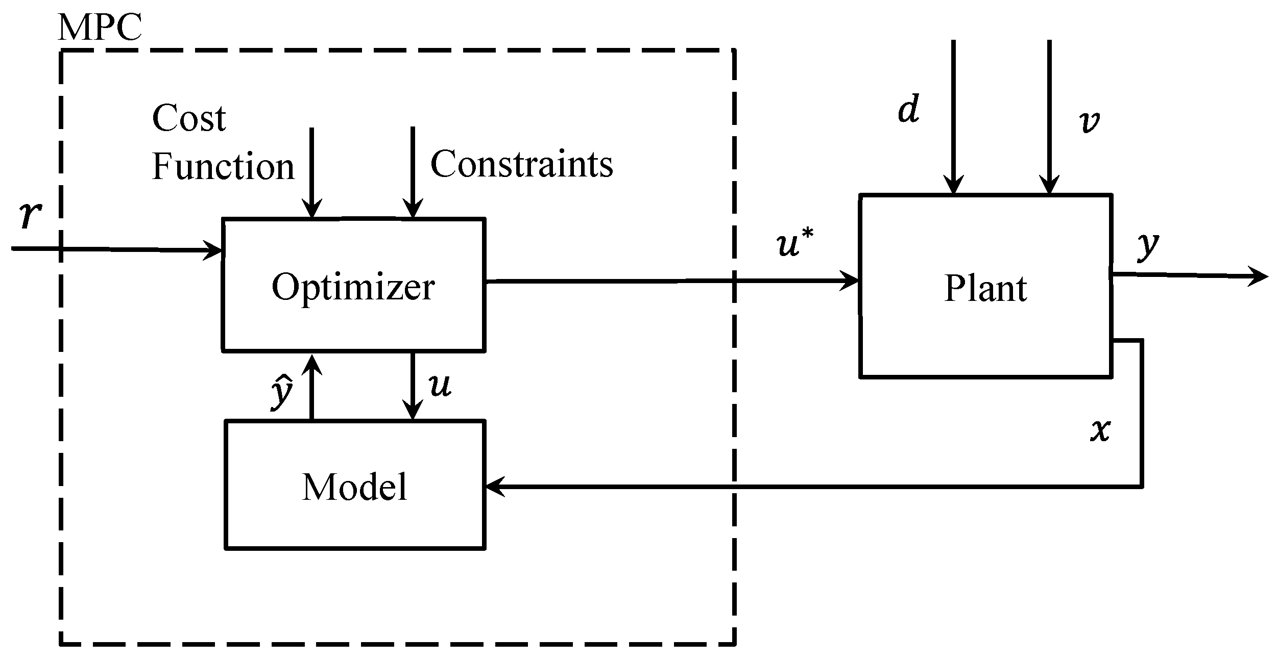
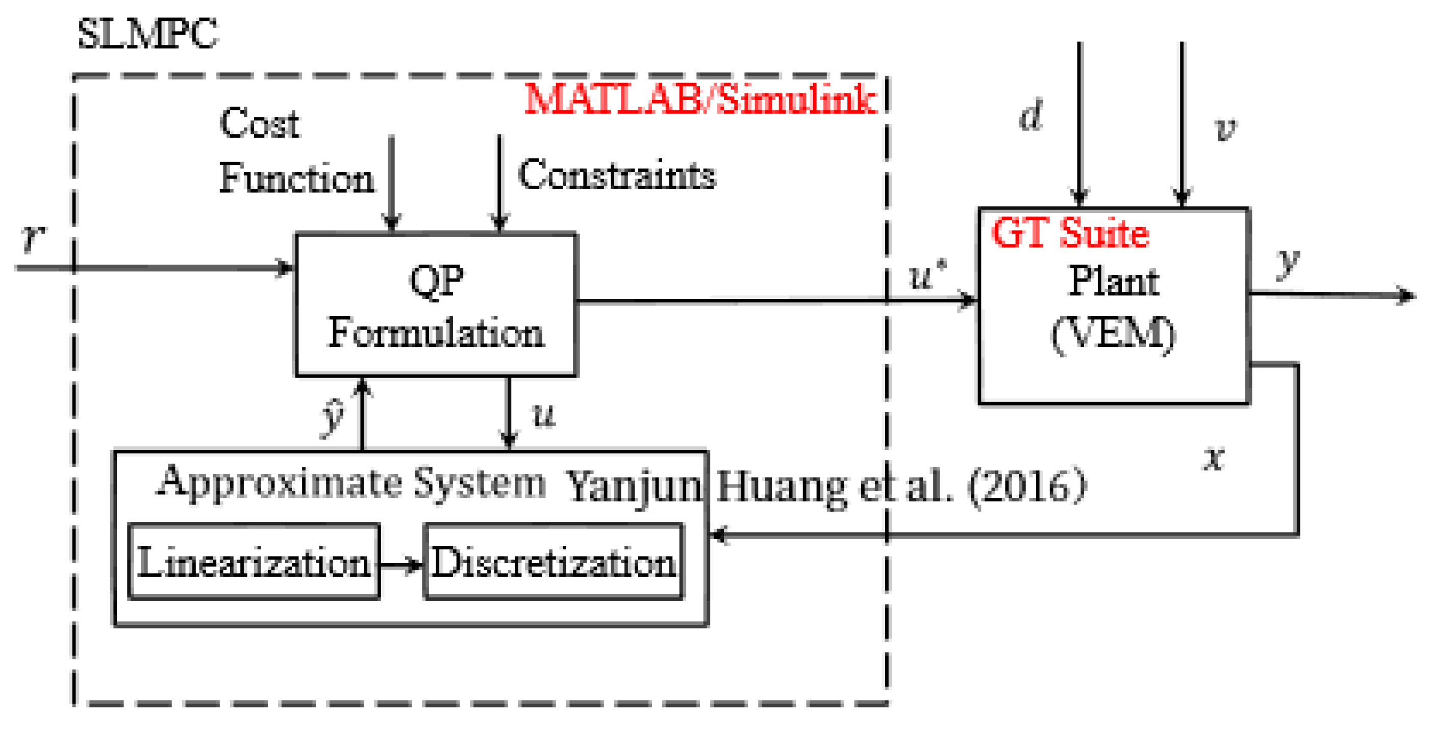
This section provides preliminary background on the theories used in this paper to help the reader follow the content more easily and to make the paper self-contained. Additionally, it provides the implemented methodology for the controller design and formulation based on the materials to help the reader follow the content with ease.

2.1. MPC Design

Model predictive control is an optimal control technique that leverages a precise mathematical model of a real system to proactively predict its future behavior. This predictive capability empowers MPC to anticipate potential system deviations and effectively optimize control inputs to achieve predefined performance objectives. By employing sophisticated optimization algorithms, MPC with the help of its more advanced derivatives can handle complex, nonlinear engineering systems with a high degree of accuracy and robustness, making it a valuable tool for a wide range of engineering applications. MPC’s ability to incorporate constraints on both system states and control inputs ensures safe and reliable operation, even in the presence of uncertainties and disturbances. Its adaptability to various real-world scenarios, such as process control, robotics, and energy management systems, underscores its versatility and practical relevance. The combination of predictive modeling, optimization, and constraint handling renders MPC an essential asset in the pursuit of efficient and stable control solutions for complex engineering systems. A simple block diagram of an MPC is shown in Figure 1, where the dashed box includes the MPC components and their interactions, namely the Optimizer block and the Model block. The model block, also known as the prediction model, contains a simplified mathematical model of the real system (plant). The prediction model computes the predicted output, y ^ . The optimizer block contains an optimization algorithm used to determine the optimal control input u based on the error predicted by the prediction model. The details of the optimizer block in this work are outlined in Section 3.3. When the optimizer computes a control signal, it sends it to the prediction model and the behavior of the real system is predicted again. This process repeats several times over an optimization window, called the prediction horizon, to forecast the future behavior of the real system. When the entire control sequence is completed, only the immediate next control action, u * , is sent to the real system with the states x and output y , designated as the plant block in Figure 1.
The plant can be a real physical system, such as a physical vehicle, or a virtual representation of the system, such as a high-fidelity model of a physical vehicle. In this paper, the plant is a high-fidelity model, introduced in Section 2.3. The connection to the real system in this work is detailed in Section 3.1 based on the previous work by the authors [28].

2.1.1. Type Selection

Selecting the appropriate MPC technique based on the system’s characteristics is an important task in the overall MPC design process. A linear time-invariant MPC method is suitable for a linear system with linear constraints and a quadratic cost function. This scenario results in a convex optimization problem with a unique global optimum. Numerous numerical methods and software can be employed to solve this well-studied problem. When moving to a nonlinear system, two methods are discussed: adaptive and gain-scheduled MPC controllers. These methods rely on linearization to approximate the nonlinear system around an operating point. While effective near this point, linearization’s limitations outside this range are acknowledged.
Adaptive MPC involves computing a linear model on the fly as conditions change, updating the internal plant model for the MPC controller. This approach maintains the optimization problem structure across various operating points. Alternatively, gain-scheduled MPC involves offline linearization at multiple operating points, designing separate MPC controllers for each. While offering controller independence, this method requires managing controller switching and may demand more memory.
It is beneficial to use adaptive MPC when the optimization problem structure remains consistent across various conditions. When the structure changes, gain-scheduled MPC is preferable. However, a nonlinear system that resists accurate linearization requires nonlinear MPC. This advanced method employs a nonlinear plant model for precise predictions but solving the associated nonconvex optimization problem in real time can be challenging.
Therefore, adaptive and gain-scheduled MPC can be used for systems that can be approximated by linear models, and nonlinear MPC can be employed for highly nonlinear systems. The implementation efficiency of nonlinear MPC must be considered as it relies on specialized nonlinear solvers.
The A/C system used in this study was developed and published by the authors of this study in [28]. This model is an extension to a previously developed model by the industrial partner’s collaborators where effects of underhood aerodynamics and modeling of system parameters using polynomial approximations are added for a more extensive and semi-analytical model of the system under study. The model in [28] requires an adaptive MPC for the control strategy development because it meets the following requirements for a choice of the adaptive MPC over a traditional MPC:
  • Time-varying dynamics: The system’s dynamics in [28] change over time due to various factors such as varying operating conditions or system wear and tear.
  • Uncertain models: Some of the model parameters [28] are not precisely known as they are embedded in the model developed by the industrial partner where the exact values of the parameters are unknown and approximate values were used to build the semi-analytical model, and there is uncertainty about the model’s accuracy.
  • Nonlinear systems: The system in [28] is highly nonlinear and for controlling systems with nonlinear behavior, where a linear model may not be sufficient, and an adaptive model helps to approximate the nonlinear dynamics better.
  • Disturbance rejection: As mentioned in item 2, some of the system parameters are not entirely known throughout the simulation as they are provided by the software-in-the-loop and depend on the driving cycle that the tests are being run over. When dealing with systems subject to disturbances that are not entirely predictable or change over time, adaptive MPC is the plausible choice.
  • Parameter variations: Some of the system parameters in [28] change over time, and their values are embedded in the software-in-the-loop provided by the industrial partner. In cases where there are abrupt changes or slow variations in system parameters, adaptive MPC can be useful.
Therefore, a variation of adaptive MPC, Successive Linearization Based Model Predictive Control (SLMPC) [29] (see Appendix A for detailed derivation), is chosen for the problem introduced in this paper due to its ability to reduce the linearization error caused by the system operating far from the trim state. In the adaptive MPC, a linear model of the system is computed on the fly as the operating conditions change and the internal prediction model is updated with each new linearized model. As the operating conditions change, only the model of the system is updated and the MPC formulation remains the same. As discussed in Section 2.3, the plant model for the A/C system used in this study has varying system parameters that are controlled by other subsystems in the vehicle, therefore making this system time-varying. The use of adaptive MPC ensures that, despite variations in system parameters, at every operating point, the linearization guarantees close agreement between the linearized model and the nonlinear plant model for the A/C system.
In addition to the type of MPC controller, there are parameters to be discussed in the design process for any MPC controller. These parameters are discussed next.

2.1.2. Design Parameters

For MPC design, there are essential parameters that require careful consideration to enhance both controller performance and computational efficiency. These parameters encompass the controller sample time, prediction horizon, control horizon, constraint handling, and weight assignment. Each parameter plays a pivotal role in optimizing the MPC algorithm’s real-time performance while ensuring effective control of dynamic systems.
  • Sample time: The choice of the sample time determines the controller’s operational frequency, impacting its ability to respond to disturbances and setpoint changes. Balancing between rapid disturbance rejection and computational load, it is advisable to accommodate 10 to 20 samples within the open-loop system’s rise time [30]. This ensures a responsive controller without overwhelming computational demands. Further details about this parameter in this study are provided in Section 3.4.2.
  • Prediction horizon: The prediction horizon influences the extent to which the controller anticipates future plant behavior. A cautious prediction horizon encompasses a timeframe that captures significant system dynamics, preventing untimely responses to disturbances. To account for open-loop transient responses, selecting 10 to 20 samples is recommended [30]. Further details about this parameter in this study are provided in Section 3.4.2.
  • Control horizon: Conversely, the control horizon determines the number of future control inputs that shape the predicted plant output. A smaller control horizon minimizes computational efforts but may compromise maneuverability. An optimal balance can be struck by setting the control horizon to 10–20% of the prediction horizon, ensuring a minimum of 2–3 steps to account for effective control [30]. Further details about this parameter in this study are provided in Section 3.4.2.
  • Constraints: Constraints on inputs, input rate changes, and outputs can be imposed within the MPC framework. These constraints may be either hard or soft. The distinction lies in the feasibility of violation: hard constraints remain inviolable, while soft constraints can be breached within limits. Balancing the conflicting interests of inputs and outputs, it is advised to adopt soft constraints for outputs, eschewing simultaneous hard constraints on inputs and their rate of change. This minimizes the risk of infeasibility and ensures more adaptable control [30]. Further details about this parameter in this study are provided in Section 3.3 and Section 3.4.3.
  • Weights: Weight assignment is a critical aspect of optimizing control performance. Weights gauge the significance of objectives in MPC. These objectives involve tracking setpoints and achieving smooth control maneuvers. Achieving a harmonious performance balance necessitates cautiously weighing input rates and outputs relative to each other. Additionally, adjusting weights within these categories fine-tunes performance to the specific control objectives [30]. Further details about this parameter in this study are provided in Section 3.3 and Section 3.4.4.
One can see the role of distinct MPC design parameters in shaping controller efficacy and computational efficiency. By strategically tuning these parameters, control engineers can harness MPC’s potential to efficiently regulate dynamic systems while navigating the intricacies of real-time optimization.

2.2. Discrete State-Space General Form

MPC strategies commonly use discrete state-space formulations for the mathematical modeling of the system of interest. A continuous-time linear state-space model form must be discretized to form a discrete-time linear state-space model. Typically, MPC algorithms are designed in discrete time. A great amount of MPC designs have been developed using discrete-time approaches and a much smaller amount of continuous-time MPCs are present in the literature. In this work, a discrete-time MPC has been chosen due to the nature of the communication between the MPC and the real system, as discussed in Section 3.1.
The standard form of a continuous state-space system can be written as [31]:
x ˙ = A x + B u y = C x + D u
where A , B , C , and D are matrices describing the system dynamics. x is the state vector, u is the controlled input vector, and y is the output vector.
The continuous system in (1) can be written in a discrete state-space system as [32]:
x k + 1 = A d x k + B d u k y k = C d x k + D d u k
where A d , B d , C d , and D d are matrices describing the linearized system dynamics. k denotes the current timestep, x k is the state vector, u k is the controlled input vector, and y k is the output vector. One can use forward Euler’s method to convert (1) to (2).
Forward Euler’s method is a simple discretization method for continuous-time systems. It is based on the approximation of the first derivative at t = k T where T is the time step for the discretization. Having [31]
x ˙ t = d x t d t 1 T x k + 1 T x k T
Applying the approximate formula in (3) to the SSR system equation, we have [31]
1 T x k + 1 T x k T A x k T + B u k T x k + 1 T I + T A x k T + T B u T
or [31]
x k + 1 I + T A x k + T B u k x k + 1 A d x k + B d u k
where A d = I + T A and B d = T B are the discrete system matrices for the discrete SSR of the system with sampling time T . The same approach can be followed to obtain C d and D d that similar to B d would only have a multiplication by T . The sampling time for the discretization in this study was chosen as T = 1   s as detailed in Section 2.1.2. In this paper, the system equations of the dynamics of an automotive A/C system, as detailed in Section 2.3, are considered. These equations are nonlinear and, therefore, are linearized to conform to the standard continuous-time form in (1). These continuous-time equations are then discretized to conform to the discrete-time form in (2) using the forward Euler method. The details of the full process are described in Section 3.

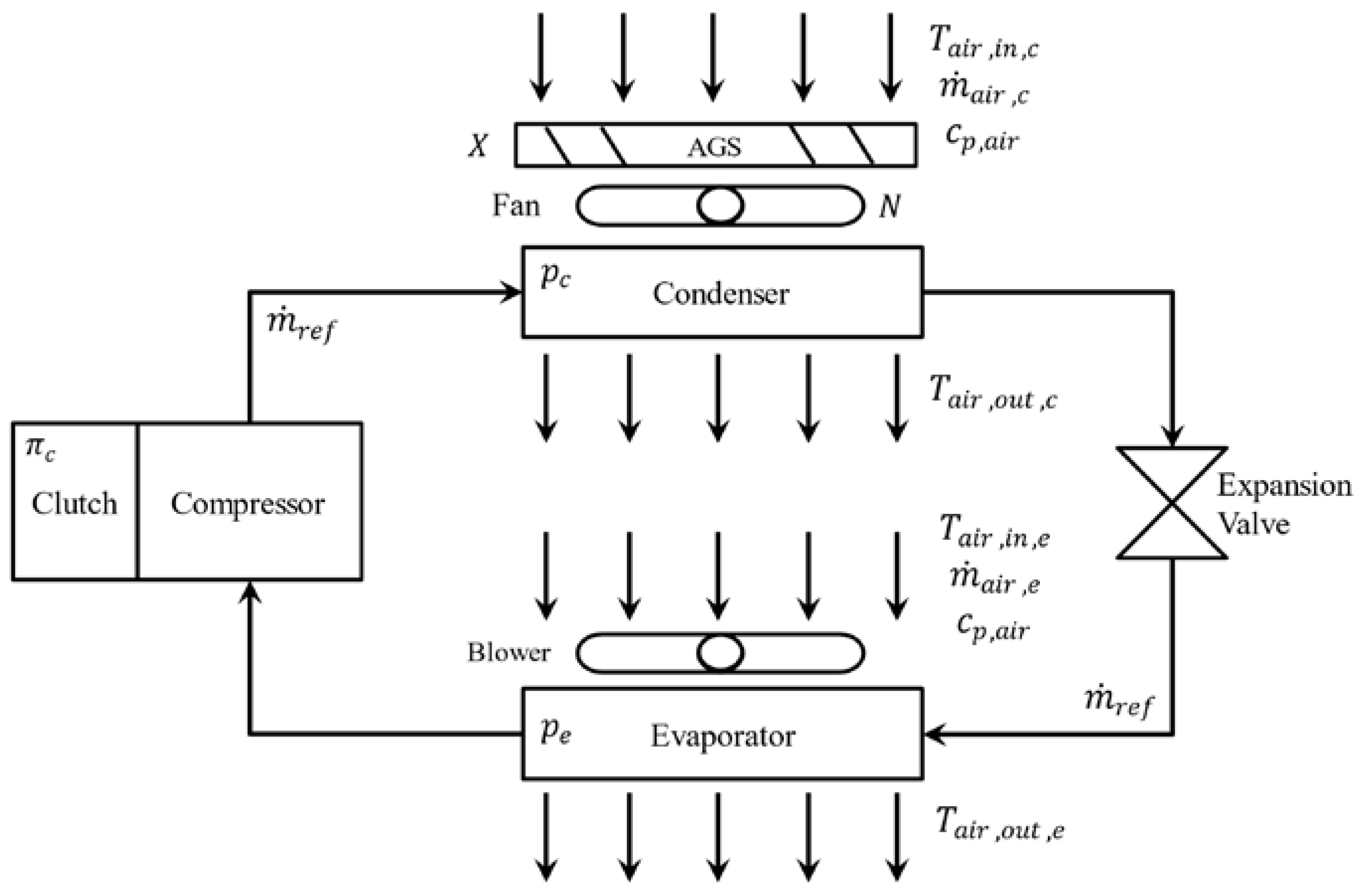
2.3. Introduction of A/C System

A simple diagram of the automotive A/C system used in this study is depicted in Figure 2. The A/C system comprises four main components, the compressor, condenser, evaporator, and expansion valve. The controllable actuators of interest in this work are the compressor clutch, which switches the compressor (used to move the refrigerant throughout the cooling circuit) on and off, and the fan and AGS used to regulate the front-end airflow passing through the condenser. Compressor clutch π c is not a continuous variable in practice and is a discrete binary variable as either engaged (with the value of 1) or disengaged (with the value of 0). In this study, π c is initially treated as a continuous variable to be computed via optimization. When the MPC computes the continuous compressor clutch signal π c , it rounds it to a value of either 0 or 1 prior to sending it to the GT-Suite model to ensure it is in the discrete form that GT-Suite expects (see Appendix B for a discussion on MPC relaxation and justification for applicability of this approach in this context).
The model used by the MPC is a semi-analytical nonlinear model of the A/C system by Parent et al. [28] (the authors of this study) as a prerequisite to run this study for controller design development. The dynamics of this model can be described by the heat exchanger pressures p c for condenser and p e for evaporator. The first system output of interest is the temperature of the evaporator air stream. The underlying continuous-time mathematical equations for the heat exchanger pressures and temperatures are [28]:
p ˙ c = Q c ρ a c p , a i r T a i r , i n T a i r , o u t + π c m ˙ r e f h i n h o u t V 1 γ ¯ ρ l h l p + γ ¯ ρ g h g p + ρ g h g ρ l h l γ ¯ p 1 + m H c H V T w a l l p p ˙ e = Q e ρ a c p , a i r T a i r , i n T a i r , o u t + π c m ˙ r e f h i n h o u t V 1 γ ¯ ρ l h l p + γ ¯ ρ g h g p + ρ g h g ρ l h l γ ¯ p 1 + m H c H V T w a l l p T a i r , o u t , c = T r e f , c + T a i r , i n , c T r e f , c N T U c K c a T a i r , o u t , e = T r e f , e + T a i r , i n , e T r e f , e N T U e K e a N T U = α A s 1 F f i n 1 η F A m ˙ a c p , a i r
where Q c is the volume flow rate of the air through the condenser [ m 3 / s ] , ρ a is the air density [ k g / m 3 ] , h i n and h o u t are the inlet and outlet refrigerant enthalpies [ j o u l e s ], ρ l , ρ g are the densities [ k g / m 3 ] and h l , h g are the enthalpies [ j o u l e s ] for the refrigerant calculated at saturated liquid and vapor states, respectively. c H is the specific heat of the HEX material [ j / K · k g ], c p , a i r is the specific heat of air at constant pressure [ j / K · k g ], γ ¯ 0 ,   1 is the mean void fraction of the refrigerant, V is the volume of the HEX [ m 3 ], m H is the material mass of the HEX [ k g ], T w a l l is the wall temperature of the HEX [ K ], p c and p e are the refrigerant pressures in the condenser and evaporator [ k P a ], π c is the compressor clutch engagement [on/off], m ˙ r e f is the refrigerant mass flow rate [ k g / s ], Q e is the volume flow rate of the air from the blower fan [ m 3 / s ], T a i r , i n and T a i r , o u t are the inlet air temperatures to the condenser and evaporator [ K ], T r e f is the HEX refrigerant temperature [ K ], N T U is the number of transfer units of the air, and K c a and K e a act as multipliers on the Nusselt number. α is the convective heat transfer coefficient of the air [ W / m 2 · K ], A s is the external surface area of the HEX [ m 2 ], F f i n 0 ,   1 is the fraction of air-to-structure surface area on the fins, η F A is the air-side fin efficiency, and m ˙ a is the mass flow rate of the air [ k g / s ].
From the developments in [28], the definitions for Q c and T r e f , c in continuous time are as follows:
Q c = 0.07722 N ^ + 0.01057 v + 4.913 × 10 5 v 2 + 0.2039 X N ^ + 0.002671 X v T r e f , c = 8.4 · 10 9 p c 3 4.9 · 10 5 p c 2 + 0.12 p c 34.9
where N ^ is the normalized rotational speed of the condenser fan between zero and one, X is the open-fraction of the AGS between zero and one, and v is the vehicle speed [ m / s ]. The full list of fitted curves is available in Appendix A of [28] in equations (17)–(20) and not further provided here for brevity.
Note that, in the system model in (6), there are terms that are updated from outside of the A/C system model and controller by other vehicle subsystems. These parameters are updated as the vehicle is operating and not controlled by the controller designed in this study for the A/C system. Hence, they are treated as system parameters in (6) that vary with time. The varying system parameters controlled by other subsystems in the vehicle dynamics are defined as follows:
θ = m ˙ r e f Q e T a i r , i n , c T a i r , i n , e h i n , c v h i n , c o m p = θ 1 θ 2 θ 3 θ 4 θ 5 θ 6 θ 7
where m ˙ r e f is the mass flow rate of the refrigerant set by the compressor in GT-Suite [ k g / s ], Q e is the volumetric flow rate of the air set by the evaporator blower model in GT-Suite [ m 3 / s ], T a i r , i n , c and T a i r , i n , e are the air temperatures entering the condenser and evaporator [ K ], h i n , c is the inlet enthalpy for the condenser [ j o u l e s ], v is the vehicle speed [ m / s ], and h i n , c o m p is the inlet enthalpy for the compressor [ j o u l e s ]. All these parameters are measured and sent from the vehicle energy management (VEM) model to the MPC. It is important to note that this makes the system under study a nonlinear time-varying system, which would require an adaptive MPC type to handle the nonlinearities by linearizing the model at each operating point, as discussed in Section 2.1.1.
Since system energy consumption is of interest, the model includes the power consumption definitions in continuous time as [28]:
W ˙ c o m p = m ˙ r e f h o u t h i n η c o m p W ˙ f a n = Q c Δ p t η f a n W ˙ d r a g = 1 2 ρ a A f r v 3 C d g 2 = W ˙ t o t a l = W ˙ c o m p + W ˙ f a n + W ˙ d r a g
where W ˙ c o m p is the compressor’s power consumption [ j / s ], W ˙ f a n is the fan’s power consumption [ j / s ], and Δ W ˙ d r a g is power consumption associated with additional drag on the vehicle due to underhood airflow, which is set by the vehicle speed, fan rotational speed, and AGS open-fraction [ j / s ]. W ˙ t o t a l is the total power consumption from A/C comprising of the previous three components [ j / s ]. m ˙ r e f is the mass flow rate of the refrigerant [ m 3 / s ], h i n and h o u t are the enthalpies of the refrigerant at the inlet and outlet of the compressor, respectively [ j / k g ], η c o m p is the ratio of isentropic efficiency to volumetric efficiency of the compressor, Δ p t is the pressure rise required of the fan [Pa], η f a n is the fan’s adiabatic efficiency, A f r is the frontal area of the vehicle [ m 2 ], C d is the increase in drag coefficient due to additional flow through the underhood at a given vehicle speed due to the AGS being open and/or the fan being on, and v is the vehicle speed [ m / s ].
With all the required background information discussed above, next, the problem definition is discussed in more detail.

3. Problem Definition

This section provides a step-by-step formulation of the problem studied in this paper.

3.1. Introduction

To conduct simulations to determine the desired MPC design parameters, the industrial partner supplied a high-fidelity model of the physical vehicle in GT-Suite v2020 (Build 3.0002), a multi-physics simulation software created by Gamma Technologies. This high-fidelity model is treated as a substitute for the real physical vehicle in this work (plant). GT-Suite v2020 (Build 3.0002) and MathWorks’ Simulink 2021b have built-in cross-platform communication capabilities that allow signals to be sent to and from the two software packages. Therefore, MATLAB and Simulink are used for the MPC implementation. In the GT-Suite model, there are numerous independent cases set up for simulation, each representing a different standard drive cycle with time-series data loaded for each of the driving conditions, some of which are the system parameters in (8) required by the MPC from GT-Suite, such as the vehicle speed. The remaining elements of (8) are computed by the GT-Suite model and sent to the MPC, such as m ˙ r e f and Q e . In this work, the MPC simulations are conducted for the SC03 drive cycle [33], which is a standard drive cycle used by the Environmental Protection Agency (EPA) to evaluate the vehicle fuel economy where the A/C system is active. The total duration of this drive cycle is 575 s.

3.2. System Equations

In this paper, an adaptive MPC, known as successive linearization-based MPC (SLMPC), is applied to the automotive A/C system illustrated in Figure 2, i.e., the A/C system is the plant. To define the elements of A , B , C , and D used in the prediction model described in (2), the system of nonlinear equations described in (6)–(9) must be linearized. These equations are linearized on the fly using the adaptive MPC approach described in Section 2.1, allowing the trim state to always be the current working state of the plant. The Jacobian matrices that map the system nonlinear equations in (6) to the linearized state-space representation A , B , C , D are calculated at every time step using the MATLAB jacobian function, where j a c o b i a n f , v computes the Jacobian matrix of symbolic function f with respect to v . The i , j element of the result of f i / v j is as follows:
A = j a c o b i a n f 1 , f 2 , x 1 , x 2 B = j a c o b i a n f 1 , f 2 , u 1 , u 2 , u 3 C = j a c o b i a n g 1 , g 2 , x 1 , x 2 D = j a c o b i a n g 1 , g 2 , u 1 , u 2 , u 3
where f 1 is the definition of p ˙ c , f 2 is the definition of p ˙ e , g 1 is the definition of T a i r , o u t , e in (6), and g 2 is the definition of W ˙ t o t a l in (9). x is defined in (27); u is defined in (28). Additionally, the collective terms g 1 and g 2 capture the system outputs y as defined in (29). Note that, due to the form of the definitions for f 1 , f 2 , g 1 , and g 2 , the full form of the Jacobians in (10) is not provided here as it would be infeasible to fit all the terms in a presentable format.
The numerical values of the state-space matrices are computed using a successive linearization approach [29], SLMPC, as a common approach adopted for MPC designs [34]. The concept of this approach is simple. At the beginning of each control iteration, the Jacobian matrices are evaluated at the current operating conditions of the complex system model, that being the current system states, controlled inputs, and system parameters. This will update the numerical values of the state-space matrix entries. By re-evaluating the state-space model at the current operating conditions, one ensures that the trim state is close to the current operating point. The intention of this is to reduce the linearization error caused by deviations from the trim state. Thus, the working condition of the complex system model will be treated as the trim state. Full theoretical development and proof of applicability for SLMPC can be found in [29]. This allows the controller to be initialized at the current system state at each time step, allowing accuracy to be maintained throughout the simulation since the controller will always work in the vicinity of the calculated trim state.

3.3. Quadratic Programming Formulation

Quadratic programming is an optimization process used to solve mathematical problems containing quadratic functions. The optimal solution to a quadratic programming problem is found by minimizing the following objective function, J [32]:
J = m i n 1 2 X q p T H X q p + f T X q p
where X q p is a vector containing the control objectives shown in (12), H is a symmetric matrix containing relative weightings for each control objective in the quadratic term of the cost function, and f is a vector containing relative weightings for each control objective in the linear term of the cost function. In (11), the elements of the vector X q p are minimized to achieve the smallest possible value for the objective function.
For the MPC controllers, the controller is typically designed to track reference values for the states and outputs of the system while also considering the magnitude and rate of change of the controlled input values. In this case, the elements of X q p are as follows [32]:
X q p = u 0 x 1 u h 1 x h y 1 y h h n x + n u + n y
where the definitions of these terms are provided further below. This description of X q p is for a discrete-time case since the approach used for the controller design in this study is also discrete-time due to the nature of the controller type. The dimension of the vector depends on the prediction horizon length h , the number of states n x , number of inputs n u , and the number of outputs n y . The elements of the H matrix can be used to change the relative importance of each of the control objectives corresponding to the terms in the X q p vector as outlined in (12).
The typical state-space equations can be modified to include the output and state reference tracking deviations. This will make forming the QP constraints much easier. The goal of the following modifications to the state-space model form is to explicitly show the output setpoint deviations, state setpoint deviations, and the rate of change of the controlled inputs since these are included in the X q p vector of the objective function. In QP problem formulations, linear equality constraints containing the X q p vector can be applied to the problem. These constraints can be used to mathematically define the elements of X q p . This can be done by treating the discrete state-space model in (2) as an equality constraint and reorganizing the formulation to contain the elements of X q p explicitly. The state-space formulation described in (2) is reorganized to explicitly include the elements of (12) using the approach outlined in [32]. As a special case of the general form of the objective function for QP in (11) when H is symmetric positive-definite, the objective function reduces to J = m i n 1 2 X q p X q p , s H 2 where H = H T H follows from the Cholesky decomposition of H and f = H T X q p , s . Hence, given the system in (2), the special case of the objective function in QP can be expanded as [32]:
J = i = 1 h y k + i y k + i , s Q y 2 + x k + i x k + i , s Q x 2 + u k + i 1 R u 2 + u k + i 1 R u 2 S . t .   : D y n a m i c   M o d e l   a n d   C o n s t r a i n t s
where the subscript s denotes a setpoint, i is the current step in the time horizon window, and I is the identity matrix. Note that subscript i is from 0 to the time horizon h as the dimensions of these vectors change with the size of the time horizon. To make the formulation easier, the system equations are written in
x k + 1 = A d x k + B d u k + B d u k 1 u k = u k 1 + u k                                               y k + 1 = C d x k + 1 + D d u k + D d u k 1
where u k   u k u k 1 . Rewriting the model in this form incorporates the rate of change of the controller inputs into the state-space model. The next step is to rewrite the state-space model in terms of setpoint deviations. So, the general form of the model equation becomes:
x k + 1 x k + 1 , s = A d x k x k , s + A d x k , s + B d u k + B d u k 1 x k + 1 , s u k = u k 1 + u k y k + 1 y k + 1 , s = C d x k + 1 x k + 1 , s + C d x k + 1 , s + D d u k + D d u k 1 y k + 1 , s
Or in a compact form as
x k + 1 x k + 1 , s u k = A d B d 0 n u × n x I n u × n u x k x k , s u k 1 + B d I n u × n u u k x k , s 0 n u × 1 + A d B d 0 n u × n x I n u × n u x k , s 0 n u × 1 y k + 1 y k + 1 , s = C d 0 n y × n u x k + 1 x k + 1 , s u k + 0 n u × n x D d u k + 0 n u × n x D d x k x k , s u k 1 y k + 1 , s + C d 0 n y × n u x k + 1 , s 0 n u × 1
If we define
x k = x k x k , s u k 1 ,   A = A d B d 0 n u × n x I n u × n u ,   B = B d I n u × n u ,   x k , s = x k , s 0 n u × 1 y k = y k y k , s ,   C = C d 0 n y × n u , D = 0 n u × n x D d ,   Q x = Q x 0 n x × n u 0 n u × n x R u
The form in (16) can be rearranged for time step 0 in the prediction horizon, where we initiate the dynamics with x 0 , y 0 , and u 1 , and given an equality constraint can be written in the form of A e q X q p = B e q
x 1 = A x 0 + B u 0 x 1 , s + A x 0 , s y 1 = C x 1 + D u 0 + D x 0 y 1 , s + C x 1 , s A e q X q p = B e q F o r m x 1 B u 0 = A x 0 u 1 x 1 , s y 1 C x 1 D Δ u 0 = y 1 , s + C x 1 , s + D x 0 u 1      
And for any other time step between i = 1 up to h 1   it can be written as follows:
x k + 1 = A x k + B u k x k + 1 , s + A x k , s y k + 1 = C x k + 1 + D u k + D x k y k + 1 , s + C x k + 1 , s A e q X q p = B e q F o r m x k + 1 A x k B u k = A x k , s x k + 1 , s y k + 1 C x k + 1 D u k = y k + 1 , s + C x k + 1 , s + D x k      
Hence, the objective function in (13) becomes:
J = i = 1 h y k + i Q y 2 + x k + i Q x 2 + u k + i 1 R u 2 S . t .   : D y n a m i c   M o d e l   a n d   C o n s t r a i n t s
which can be written in compact form as:
J = i = 1 h X q p T H X q p                                                                                   S . t .   : A e q X q p = B e q   a n d   l b X X q p u b X
where
A e q = B I n x ; 0 0 0 0 A B I n x ; 0 0 A B I n x ; 0 0 D C 0 I n y 0 0 D C 0 I n y h n x + n u + n y × h n x + 2 n u + n y
B e q = A x 0 u 1 x 1 , s A x 1 , s x 2 , s A x h 1 , s x h , s y 1 , s + C x 1 , s + D x 0 u 1 y h , s + C x h , s + D x h h n x + n u + n y × 1
with the lower and upper bounds for the entire length of the prediction horizon as
l b = l b u u b u l b x x 1 , s l b u l b u u b u l b x x h , s l b u l b y y 1 , s l b y y h , s h n x + n u + n y × 1
u b = u b u l b u u b x x 1 , s u b u u b u l b u u b x x h , s u b u u b y y 1 , s u b y y h , s h n x + n u + n y × 1
where l b u and u b u are the lower and upper bounds on the inputs, and l b x , u b x , l b y , and u b y are the lower and upper bounds for the states and outputs, respectively. Each element of the X q p vector can be weighted individually, providing more significance to prioritizing certain control objectives over others. The weighting matrix H for the control objectives within the objective function (output reference tracking, state reference tracking, input value magnitude, and rate of change of the input commands) is [32]
H = R u 0 0 Q x 0 0 0 R u 0 0 Q x 0 0 0 0 Q y 0 0 0 Q y h n x + 2 n u + n y × h n x + 2 n u + n y Q x = Q x 0 n x × n u 0 n u × n x R u n x + n u × n x + n u
where R u is the weighting of the rate of change of the inputs, Q x is the weighting of the state reference tracking deviations, R u is the weighting of the input magnitudes, and Q y is the weighting of the output reference tracking deviations. R u , Q x , R u , and Q y are diagonal matrices with the respective weights along the diagonal.

3.4. Implementation

The cabin cooling effort of the A/C system is controlled using three actuators: the compressor clutch, π c , condenser fan, N ^ , and the AGS, X . The compressor clutch connects the compressor to the engine, enabling the compressor to operate and increase the pressure of the refrigerant leaving through the discharge port. As mentioned in Section 2.3, the compressor clutch π c is not a continuous variable in practice and is a discrete binary variable. In this study, π c is initially treated as a continuous variable to be computed via QP optimization. When the MPC computes the continuous compressor clutch signal π c , it rounds it to a value of either 0 or 1 prior to sending it to the GT-Suite model to ensure it is in the discrete form that GT-Suite expects. Alternative methods exist that are better suited for dealing with mixed-variable systems like the one described. For instance, techniques such as hybrid predictive control models that incorporate both integer and continuous variables have been explored in the literature [35,36,37,38] and can be further investigated in future studies. These methods provide a more holistic approach to dealing with mixed-variable systems, allowing for more accurate and efficient control strategies in scenarios where variables exhibit both continuous and discrete behaviors.
The condenser fan and AGS regulate the flow of the ambient air stream entering the vehicle’s front end, which passes through the condenser to exchange heat with the refrigerant. The fan’s rotational speed is continuously controllable, and the AGS area open-fraction can continuously vary between fully closed and fully open. Note that some underhood airflow can still occur when fully closed due to the vehicle’s motion and/or fan operation.
Based on the approach detailed in Section 2.2, using a time step of one second leaves only the A matrix changed due to the addition of the identity matrix, as shown in (3)–(5). By convention, the time step for MPC–plant interaction is the same as the one used within the MPC for future time predictions using the model up to the prediction horizon [32]. The time step of one second was selected after assessing the open-loop response of the air temperature output subjected to a unit step from each of the three controlled inputs for the continuous-time linear model. All other parameters, such as the external inputs, were held constant at the trim state selected based on an operating point observed for the GT-Suite (real system) model.

3.4.1. States, Inputs, and Outputs

For the simulations in this study, from the A/C system equations in (6)–(9) the state vector x is defined as:
x = p c p e = x 1 x 2
where p c and p e are the condenser and evaporator refrigerant pressures. The input vector u is defined as:
u = π c N ^ X = u 1 u 2 u 3
where π c is a continuous compressor clutch signal, N ^ is the normalized rotational speed of the condenser fan between zero and one, and X is the open fraction of the AGS between zero and one.
The output vector, y , is defined as:
y = T a i r , o u t , e W ˙ t o t a l = y 1 y 2
where T a i r , o u t , e is the temperature of the air leaving the evaporator (entering the cabin) [ K ], and W ˙ t o t a l is the total power consumption of the compressor [ W a t t ] or [ j / s ] that is comprised of W ˙ c o m p , W ˙ f a n , and Δ W ˙ d r a g , as discussed in (9). The evaporator outlet air temperature is chosen as one of the outputs for the model because the controller’s goal is to control the actuators to maintain this air temperature close to a reference or set value, thus regulating the cabin cooling performance. The other output, W ˙ t o t a l , is chosen because the second goal of this controller is to minimize the power consumption of the A/C system while satisfying the cooling objective.
It is important to note that, in the proposed formulation, feedback is taken into account by using the direct system outputs as the inputs for the controller. This means that no estimator or observer was used to obtain the state variables or the output variables of the system. In this study, it is assumed that the system outputs are measurable and noise-free, and that the system model is accurate. Therefore, a possible model mismatch is not considered.
However, in reality, these assumptions may not hold true. There may be measurement errors, nonlinearities, uncertainties, or disturbances that affect the system’s performance and stability. In such cases, using an observer or an estimator could help to improve the feedback quality and robustness of the controller. This limitation can be further explored in future studies with the implementation of an observer or an estimator to handle potential system mismatches.

3.4.2. Sampling Time, Prediction Horizon, and Control Horizon

As per the recommendations and discussion provided in Section 2.1.2, the time unit of measurement for the governing equations used to derive the linearized model is in seconds. Thus, the units of the discretization time step are in seconds to maintain consistency. The rise time of the A/C system in this study is roughly 12.7 s, meaning a time step between 0.64 s to 1.3 s would fit 10 to 20 samples within the open-loop rise time, meaning a sampling or discretization time step of T = 1 s is satisfactory based on this best practice.
As per the recommendation for the choice of prediction horizon, in this study, a prediction horizon of 10 s or 10 time steps is chosen. This reduces the computational burden for the optimization process required during the prediction horizon by choosing the lower bound of the recommended range. However, in future studies, one can further optimize the prediction horizon. Additionally, a control horizon of two steps is chosen for the implementation of the adaptive MPC as it provides a sufficient balance between computation, efficiency, and performance for the MPC design.
It should be noted that the choices above were based on trial and error in the study to obtain satisfactory results for the industrial partner in this first phase of investigations for the implementation of an MPC controller for an A/C system in a vehicle. In future studies, additional investigations shall be pursued to further improve and optimize these choices for the controller design.

3.4.3. Constraints

As discussed in Section 3.3, constraints can be set on the optimization. The values of these three controlled inputs have physical limitations based on their range of operation. These are hard constraints that cannot be exceeded by any means. The mathematical number sets and limitations of these three controlled variables are provided by the industrial partner as:
π c N s . t .                 π c = 0,1 l b u 1 ,   u b u 1 N ^ Q s . t .                 0 N ^ 1 l b u 2 , u b u 2 X Q s . t .                 0 X 1 l b u 3 , u b u 3
The states also have constraints but they are not due to physical limitations. The constraints on the states are imposed to prevent problems arising in the HEXs due to excessive or lack of pressure. The state constraints are as follows and are defined by the industrial partner:
100   kPa p e 1300   kPa l b x 1 ,   u b x 1 700   kPa p c 3000   kPa l b x 2 ,   u b x 2
For the QP algorithm to run successfully, constraints must also be present for the outputs as well but, since the outputs do not have bounds for the application in this study, they are set to infinity as
  K T a i r , o u t , e +   K l b y 1 ,   u b y 1   W a t t W ˙ t o t a l +   W a t t l b y 2 ,   u b y 2
Feasibility and infeasibility issues in MPC controllers with QP optimization can affect the stability and performance of the closed-loop system. If the QP problem has hard constraints, such as input or output limits, it may be impossible to satisfy them at some time steps, leading to infeasibility. If the QP solver detects infeasibility, it terminates immediately and returns an error in MATLAB. To avoid this situation, some methods have been proposed, such as using soft constraints, additional constraint checking horizon, terminal condition and cost, or disturbance preview [38].
In this study, the infeasibility problem shall not occur as the only hard constraints in the QP optimization in this study are on the inputs outlined in (30) and these constraints shall be met as, in any A/C system of a vehicle, there must be a combination of these inputs that provides some sort of long-term asymptotic stability and tracking for the cabin temperature even without the use of an MPC controller. This was primarily achieved by the baseline PID controlled in previous works and can be the bare minimum solution to this optimization problem that would exist at all times. Therefore, since there is no time limit on the settling time for the temperature tracking of the cabin, the control inputs and hard constraints in (30) and (31), as shown in simulation results for the ranges of p c and p e , shall not prevent the optimization problem from converging to a solution at any given time step and, hence, the infeasibility issue shall not arise.

3.4.4. Weights

Additionally, from Section 3.3, the elements of the X q p vector defined in (12) can be weighted based on importance and contribution to the objective function through the weighting matrix H described in (26). As defined in (27)–(29), for this work, there are two states ( n x = 2 ), three controlled inputs ( n i = 3 ), and two outputs ( n y = 2 ). The specific weighting matrices inside (26) are defined as follows:
Q x = K p c 0 0 K p e Q y = K T a i r 0 0 K W ˙ T R u = K π c 0 0 0 K N ^ 0 0 0 K X R Δ u = K Δ π c 0 0 0 K Δ N ^ 0 0 0 K Δ X
where K p c and K p e are the weightings for the state deviations, K T a i r is the weighting for the air temperature tracking deviation, K W ˙ T is the weighting for the total power consumption, K π c , K N ^ , and K X are the weightings for the magnitude of the controlled inputs, and K Δ π c , K Δ N ^ , and K Δ X are the weightings for the rate of change of the controlled inputs. It is worth noting that the goal of the MPC is to reduce energy consumption, but the power consumption is modeled and weighted because energy is the time integral of power. Thus, reducing power consumption will also reduce energy consumption.

3.4.5. Scenarios

Two control input cases are considered: first, only controlling the compressor clutch and, second, adding the condenser fan speed and AGS position as additional controlled inputs. Thus, the u k and u k elements of the X q p vector for the first case with clutch-only control are:
u k = π c Δ u k = Δ π c
and for the second case with full control of compressor clutch engagement, condenser fan speed, and open-fraction AGS position are:
u k = π c N ^ X ;   Δ u k = Δ π c Δ N ^ Δ X
It is important to note that, as the input vector changes in cases 1 and 2, the applied constraints in the optimization problem are also adjusted to only include the applied control inputs.

3.4.6. Summary

The overall system implementation is shown in Figure 3, where the structure of implemented SLMC is shown with notations that are the same as in Figure 1. Additionally, the environment under which each component is developed/operated is noted in red color.
To summarize this section and formalize the control problem investigated in this study, we have the continuous SSR system form in (1) that can be written in the discrete SSR system form in (2) with x defined in (27), u defined in (28), and y defined in (29). The matrices A , B , C , and D in (1) are the Jacobians calculated from (6)–(9) using (10). These matrices can be converted to their discrete form using Euler’s method described in (3)–(5) to obtain A d , B d , C d , and D d in (2) with the sampling step of T = 1   s .
The goal of the optimization problem in SLMPC is to minimize the objective function in (11) in the general case and for this study in a simplified form in (13) and with constraints formed as (21), where the elements of X q p and H are defined in general in (12)–(26) with specific definitions for this study in (33) subject to constraints in (24) and (25) in general form and for this study in (30)–(32).
Finally, the investigations are conducted for two scenarios, 1. clutch only as input for the MPC design as outlined in (34), and 2. full control input including compressor clutch engagement, condenser fan speed, and open-fraction AGS position as outlined in (35). The time or prediction horizon for the MPC design was set to 10 time steps, and since the time step for this study was chosen as T = 1   s it would equal a 10 s look ahead in time for the controller.
The results and analysis of the simulations with the VEM model, which was provided by the industrial partner in the GT-suite environment and is used as the plant for the simulations, are presented in Section 4, including some discussions on the observations made from the outcomes.

4. Results and Discussion

To evaluate the performance of the air temperature tracking, the root mean squared error (RMSE) between the actual air temperature from the GT-Suite model and the target reference temperature was calculated as:
R M S E = i = 1 n p o i n t s x a c t u a l , i x r e f e r e n c e , i 2 n p o i n t s
where x a c t u a l , i is the actual value from the GT-Suite model, x r e f e r e n c e , i is the target reference value, and n p o i n t s is the total number of data points. The choice for the performance evaluation in (36) is to ensure that the tracking of the reference value is monitored and considered throughout the entire simulation, not just for a portion of it. That is why the summation in (36) is from 1 to the total number of data points or simulation outputs.
The performance of the GT-Suite model with the baseline PID control scheme is shown in Table 1, where n Δ π c is the clutch actuation frequency in the number of actuations per minute. These metrics will be referenced to the MPC results to compare the improvement of the new control scheme.

4.1. MPC Tuning Process

The weighting parameters of the MPC controller are set for the individual elements of the objective function as X q p , defined in (12). The most crucial elements of (12) to be minimized are (i) the air temperature setpoint deviation corresponding to K T a i r in (33), (ii) the instantaneous power consumption corresponding to K W ˙ T in (33), and (iii) the rate of change of the clutch command corresponding to K Δ π c in (33). The rate of change of the clutch command is critical to consider since the durability of the compressor can be a concern if a chattering phenomenon occurs, where the compressor clutch is constantly cycled between engaging and disengaging. Wear and tear on the compressor clutch can lead to reliability issues within vehicles and can increase expenses if the compressor requires maintenance more frequently. To quantify the actuation frequency of the clutch, the total number of clutch actuations throughout the cycle is recorded and divided by the 9.583 min (575 s) duration of the test cycle used in this study. With these three as the crucial weightings of interest for the MPC tuning, all other weightings in (33) are set to a value of one, while these three ( K T a i r , K W ˙ T , and K Δ π c ) are varied to ensure a reasonable contribution of various terms in the objective function.
There are optimal methods for tuning MPCs, as reported by Vazques et al. [39] using an artificial intelligence approach for real-time tuning of MPC for power converters and by Yamashita et al. [40] using a multi-objective tuning technique for MPC tuning in grinding circuits. However, in this study, a variation in the preliminary optimization method known as grid search with a systematic distribution of the grid points in the desired search space was considered as the focus of this study was more on the feasibility of implementing an MPC controller for the vehicle’s A/C system rather than optimizing it. More advanced and optimal tuning techniques can be considered in future studies. A preliminary sensitivity assessment was conducted to determine the search space ranges for these three weighting values, K Δ π c , K T a i r , and K W ˙ T , to ensure the entire relevant search space is being explored. K Δ π c , K T a i r , and K W ˙ T were systematically increased while all other weighting factors were held constant. For example, K Δ π c was increased until no further significant change was observed in the system’s clutch actuation frequency.
To form the optimization search space, the valid weighting ranges for K Δ π c was identified as 1–1000 since values greater than 1000 presented no change to the clutch actuation frequency. The valid weighting range for K T a i r was chosen between 1–50, as the values above this range provided no significant change to the air temperature’s RMSE. Finally, the valid weighting range for K W ˙ T was chosen to be between 1 and 50 since integer values greater than 50 caused the compressor to shut off completely for the entire cycle, meaning the A/C system was inactive, and the air temperature’s RMSE reached extreme and unrealistic values. Therefore, the optimization process for the MPC tuning could be described as
m a x i m i z e ( or   minimize )   f G S K Δ π c , K T a i r , a n d   K W ˙ T   subject   to   1 K Δ π c 1000 1 K T a i r 50 1 K W ˙ T 50
where f G S · is the function whose value needs to be maximized or minimized during the optimization process. A Latin Hypercube Sampling (LHS) approach outlined by Huntington and Lyrintzis [41] was used to determine the grid points (candidate solutions distribution) in the search space for the three MPC weightings within the defined search spaces in (37). A sample space of 300 unique combinations of weighting values was randomly generated in MATLAB using LHS to adequately fill the search space defined in (37). The MPC was simulated with the GT-Suite model in two different scenarios discussed in Section 3.4.5 for the SC03 cycle. The plant was operated with the MPC for each set of 300 weighting combinations to assess the system’s behavior with the new control scheme.
As stated earlier, the three main metrics of interest are (i) the RMSE for the air temperature setpoint deviation, (ii) the total energy consumption throughout the cycle, and (iii) the clutch actuation frequency, each of which could be considered as the definition of f G S · in (37). In a traditional approach to grid search optimization, one would minimize or maximize the value of f G S · in (37) as one of the metrics outlined above. However, in this study, to provide a more insightful illustration of how the samples in the search space in (37) compare to one another against any of the above metrics, the results of the evaluation for all samples in the search space in (37) against all metrics above are shown in Figure 4. To further discuss the optimum points for this optimization approach, the points of interest (POIs) are introduced next to provide trade-offs and decision-making recommendations once the outcomes of all evaluations are obtained and visualized.

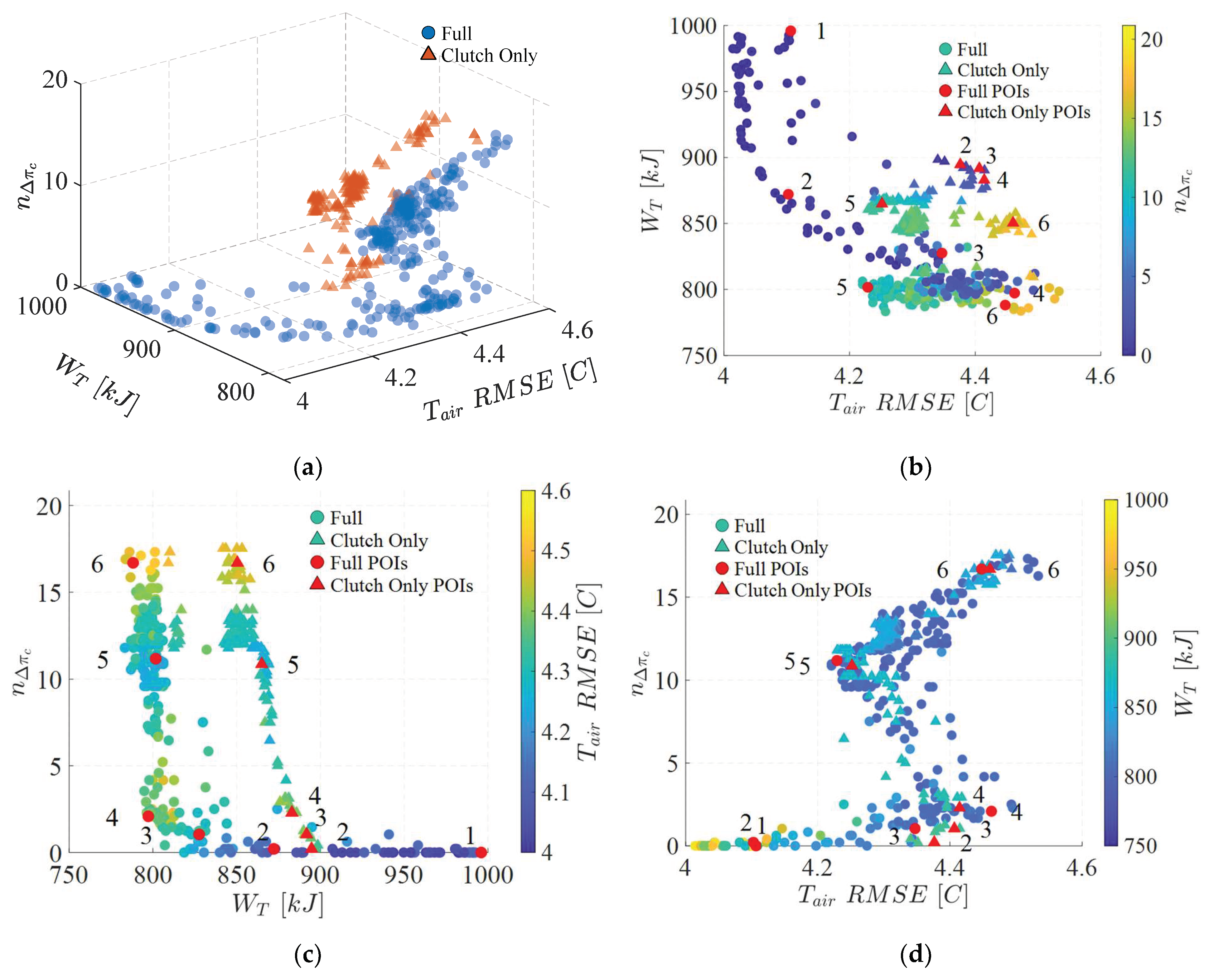
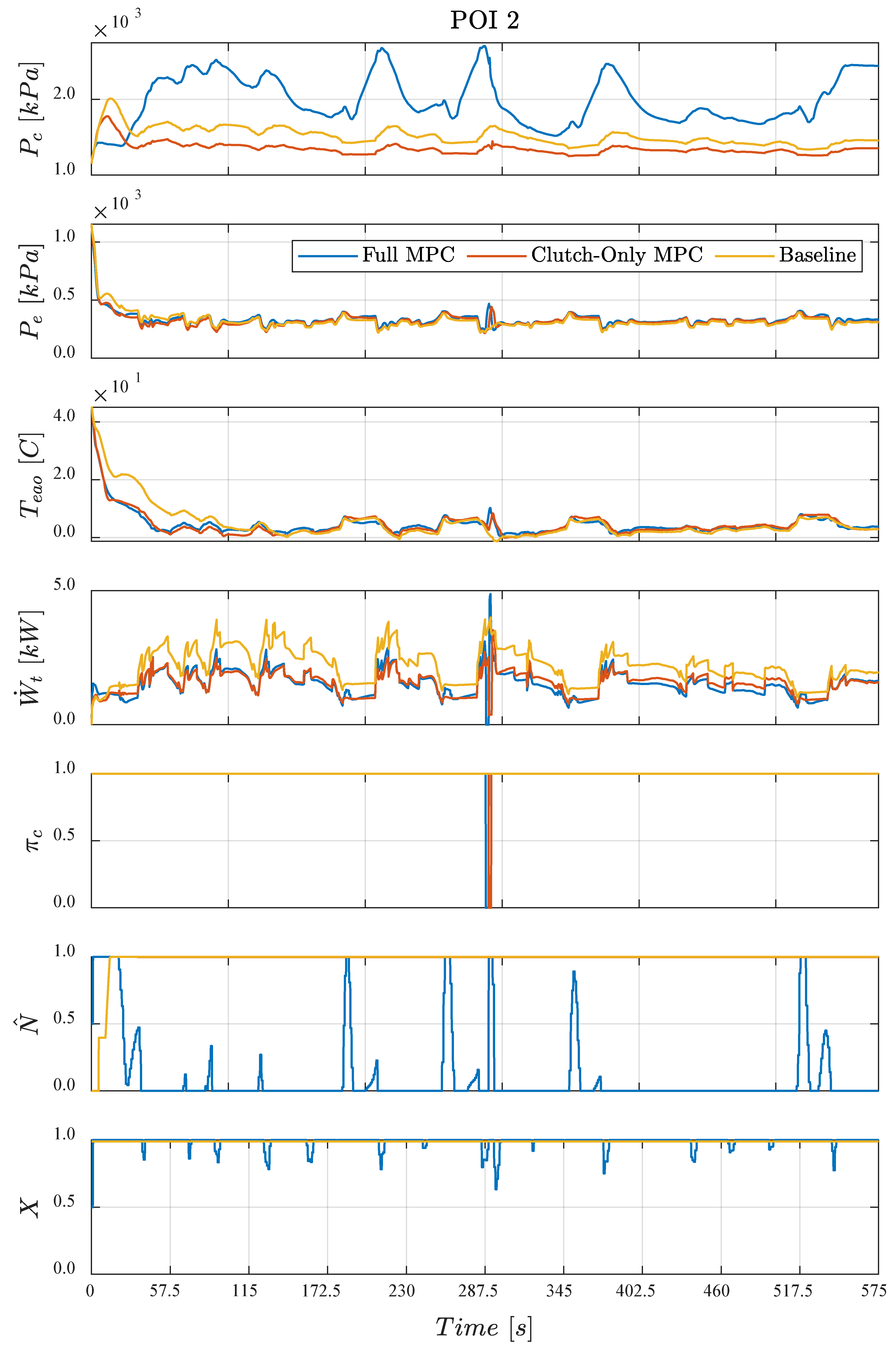
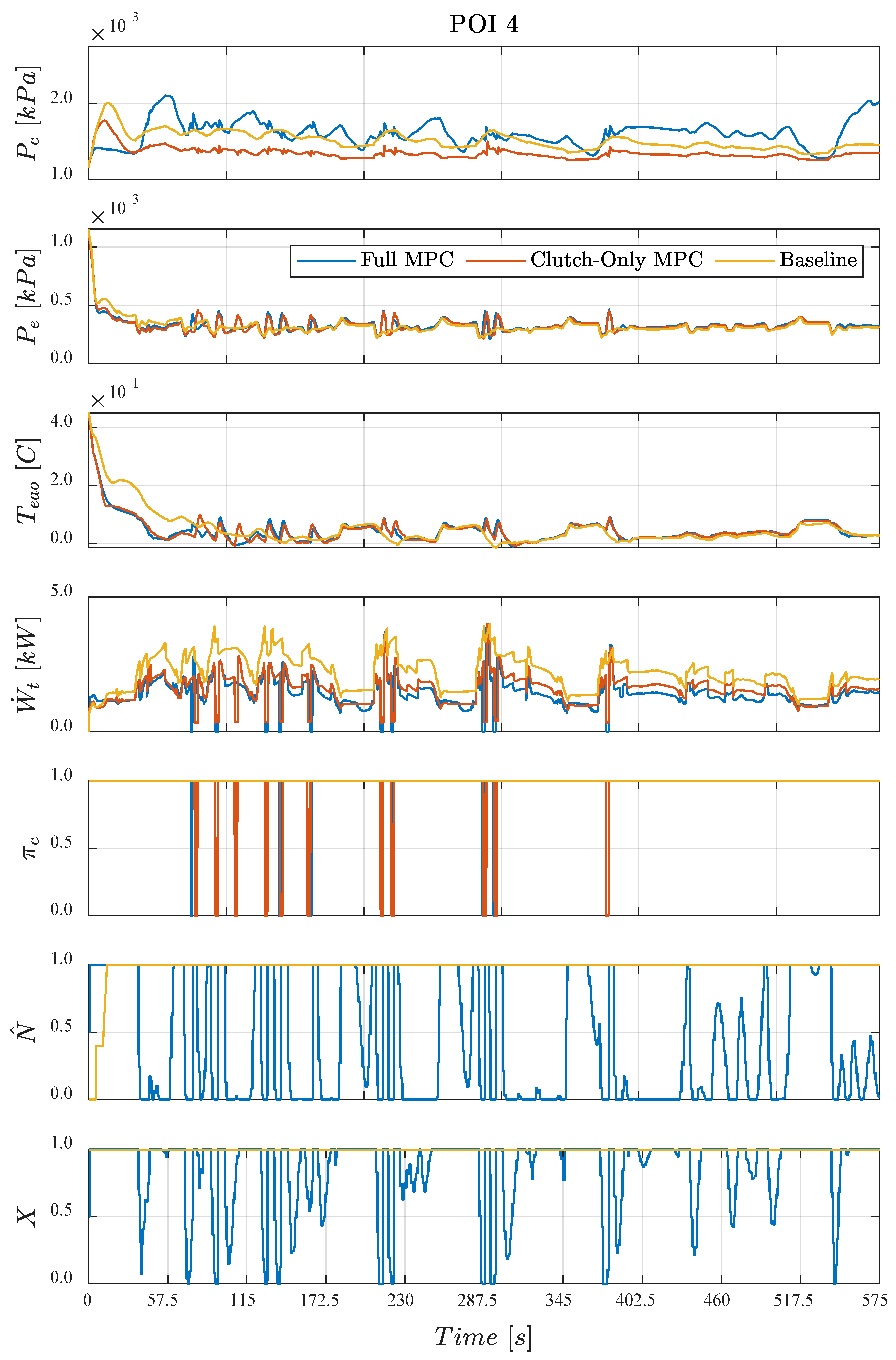
4.2. Points of Interest

First, we examine the three metrics of interest for both MPC configurations, as shown in Figure 4a. Four observations can be made here.
  • First, the upper bound of energy consumption is 1000 kJ, 21% lower than that for the baseline control scheme for the plant. Hence, all assessed MPC configurations significantly reduce A/C system energy consumption.
  • Second, in a similar way, the largest air temperature error is 4.6 ° C , 27% less than that for the baseline controls. This suggests that the model being re-linearized at every operating point is key to good control performance, as the baseline controls do not include this.
  • Third, clutch actuation frequency ranges from 0 (same as baseline) to ~16 actuations per minute over the SC03 cycle, with higher clutch actuations, in general, being traded for lower energy consumption. This suggests there is no single optimal value of the QP weights but rather a trading relationship the control designer must choose within.
  • Finally, the difference between the total energy consumption using clutch-only MPC and full MPC is apparent, with clutch-only MPC yielding higher energy consumption. The impact of the inclusion of two extra actuators into the MPC framework is easier to establish by examining the same data in each of the three two-dimensional views in Figure 4b–d.
In Figure 4b, the data is projected onto the energy–temperature error plane. It is clear that including all actuators in the MPC framework lowers energy consumption for a given temperature error at a comparable or lower clutch actuation frequency. Giving the MPC the control ability over all actuators also enables higher-energy solutions with few to no clutch actuations, which is impossible with clutch-only control.
In Figure 4c, the data is projected onto the clutch actuation frequency–energy plane. The three-actuator MPC is shown to lower energy consumption by 50–100 kJ over the drive cycle at comparable numbers of clutch actuation frequency and again the higher-energy solutions with little to no clutch activation are apparent. In Figure 4d, the data is projected onto the clutch actuation frequency–temperature error plane. Here, it can be readily seen that the three-actuator MPC enables similar temperature errors and clutch actuation frequency but at reduced energy.
Some POIs are gathered in Table 2. When the clutch does not actuate in POI 1 for full control, the energy consumption is at its highest. However, the air temperature’s RMSE is at its lowest. This scenario is most similar to the baseline control since the built-in compressor displacement control is the main driving force for the refrigerant control. As the compressor is active during the entire cycle, the energy consumption is high since the compressor is the primary energy consumption for the A/C system. Comparing this POI with the baseline performance, the energy consumption is reduced by 20.9% and the air temperature’s RMSE is reduced by 34.6%. This demonstrates that, by just using MPC control of the compressor, fan, and AGS, there is a significant improvement to the reference temperature tracking and energy consumption.
For the clutch-only control results, the smallest clutch actuation frequency was found to be 0.2, meaning the clutch has at least one on/off actuation over the 575 s drive cycle. This can possibly be attributed to the fact that the baseline fan and AGS control inside the GT-Suite model are poor, typically running the fan when it is not needed for additional cooling and maintaining the AGS fully open regardless of the cooling requirement, causing the clutch to be more inclined to be the primary source of cooling regulation.
An interesting impact can be observed by increasing the compressor clutch actuation frequency by a small margin, from POI 1 to POI 2 and 3, which is performed by decreasing the weighting value of K Δ π c or increasing the weighting values of K T a i r and K W ˙ T . For full control, by increasing the actuation frequency from zero to 0.2, the energy consumption is decreased by 30.9% compared to the baseline. Similarly, from an actuation frequency of zero to 1.01, the energy consumption is reduced by 34.5% compared to the baseline. However, the RMSE for the air temperature is increased from 4.10 °C to 4.35 °C. POIs 5 and 6 demonstrate that, when the compressor clutch actuation frequency is above 2.03 for full control, no significant improvement to the energy consumption is achieved. However, in this region, the best air temperature’s RMSE is found between a clutch actuation frequency of roughly 9.6–11.2. Comparing the POI results between the full control and clutch-only control clearly shows that, at the same clutch actuation frequency, the control of the fan and AGS provides an additional benefit to power consumption and air temperature tracking. The largest difference between the full and clutch-only control can be seen by comparing both cases at POI 3, where the full-control MPC uses 9.7% less energy compared to the clutch-only control for the same clutch actuation frequency. The weights associated with the POIs gathered in Table 2 are shown in Table 3.
The system behavior for POIs 2 and 4 are shown in Figure 5 and Figure 6, respectively, where they are both compared to the baseline system behavior. By investigating the behavior of the clutch-only MPC results shown in Figure 5 and Figure 6, it can be immediately observed that the condenser fan rotational speed and AGS open fraction are controlled in the same manner as the baseline.
The impact of the full MPC on energy consumption can be recognized by comparing the condenser fan and AGS control to the baseline. For example, in POI 2, the full MPC is able to completely shut off the condenser fan for the majority of the cycle. In order to cause a sharp increase in air temperature, the clutch is disengaged, allowing the system to heat up quickly. However, when doing so, the full MPC controller drives the rotational speed of the condenser fan to its maximum value so as to not cause a significant overshoot in air temperature. This can be seen more often in POI 4, where the clutch actuation frequency is higher. In doing so, more energy is saved by disengaging the clutch and allowing the other two actuators to work toward satisfying the air temperature reference tracking objective. In POIs 5 and 6, the clutch actuation frequency is significantly higher than in POI 4, as seen in Table 2.
The key takeaway is that there are multiple combinations of the weighting parameters which yield good performance, trading mainly between energy consumption and clutch actuation frequency. Choosing one is the designer’s job, depending on the balance desired between energy use and clutch/compressor life longevity. For the vehicle of interest in this work, the fuel economy is 9.8 L/100 km when the A/C system is not active. In terms of fuel economy, the A/C system can typically use roughly 1.0 L/100 km, increasing the fuel consumption to 10.8 L/100 km [42]. In this work, the greatest observed energy savings by the full MPC is 37.6%, which would reduce the fuel economy number to 10.4 L/100 km, roughly yielding a 3.5% savings in fuel economy.

5. Conclusions and Future Work

In this paper, two MPC schemes were applied to the A/C system of a vehicle, that is, one controlling only the compressor clutch and one additionally controlling the condenser fan and AGS. The analysis showed that, by switching to MPC control, an improvement of 32.7% to the air temperature reference tracking and 37.6% to the energy consumption can be achieved. By disengaging the compressor when it is not needed, up to 37.6% in energy savings was recorded using the full-control MPC. However, achieving a steady-state solution at the air temperature setpoint of 4 °C was not achievable by controlling the fan and AGS alone, leading to a cycling behavior of the discrete compressor clutch. By increasing the actuation frequency of the compressor clutch from zero to 2.03, the energy benefit using the full-control MPC was improved from 20.9% to 36.9%. However, increasing the clutch actuation frequency further resulted in no further energy benefit. Nevertheless, the air temperature RMSE was improved by 5.4% by increasing the clutch actuation frequency from 2.03 to 10.7, at the expense of more wear and tear on the clutch itself.
From the analysis done in this work, it can be concluded that switching to an MPC scheme is worthwhile for A/C system control, even if there is no change in the components being actuated. This can be seen by the energy saving and air temperature tracking benefit of 32.6% and 32.2% provided by the clutch-only MPC. Further benefit can be obtained, especially in terms of clutch durability, by including all three actuators in the MPC scheme. The full-control MPC is able to provide a 34.5% energy benefit with a clutch actuation frequency of 1.01, whereas the clutch-only control provides a 32.7% energy benefit with a clutch actuation frequency of 16.2. The discrete number of points investigated in the Latin Hypercube Sampling did not permit formal identification of a Pareto front. However, the trades seen between the outputs strongly suggest such a front could be identified for any given vehicle; thus, optimal weightings could be chosen based on the designer’s choice between clutch actuation frequency, energy consumption, and temperature error.

Author Contributions

Conceptualization, T.P., J.J.D. and A.R.; methodology, T.P., J.J.D. and A.R.; software, T.P. and A.R.; validation, T.P., J.J.D. and A.R.; formal analysis, T.P. and A.R.; investigation, T.P.; resources, J.J.D. and A.R.; data curation, T.P.; writing—original draft preparation, T.P.; writing—review and editing, J.J.D. and A.R.; visualization, T.P. and A.R.; supervision, J.J.D. and A.R.; project administration, J.J.D. and A.R.; funding acquisition, J.J.D. and A.R. All authors have read and agreed to the published version of the manuscript.

Funding

This research was funded by Mitacs Canada and Stellantis Canada, grant number IT25381.

Data Availability Statement

Data are contained within the article.

Acknowledgments

We thank Kevin Laboe, Nandan Sawkar, and Hamed Kharrati for supporting this work by providing insight, experimental data, and guidance.

Conflicts of Interest

The authors declare no conflicts of interest.

Appendix A. Successive Linearization Based MPC

Traditional MPC relies on discrete-time linear models, but most dynamic systems are nonlinear and continuous. To address this, one approach is to employ successive linearization. This involves linearizing the continuous nonlinear system at each sampling time around the current state, discretizing it, and using the resulting model to predict future values. A QP problem is then formulated to find a control sequence that minimizes a cost function. See Figure 3 for an illustration of this MPC approach based on successive linearization. The contents of this appendix are adapted from [29] for completeness of the presented work in this study.

Appendix A.1. Continuous Nonlinear System Linearization

Consider n x , n u , and n o , as states, inputs, and outputs of a system, respectively resulting in state x R n x , input u R n u , and output y R n o vectors. The outputs y i and states x i would be expressed as y i = z i x , u , i = 1 , . . , n o and x i ˙ = f i x , u , i = 1 , . . , n x . The system dynamics in SSR form would be
x ˙ = F x , u , y = Z x , u
Generally, the states and inputs in (A1) can be constrained as x l x x u with the lower and upper bounds as x l , x u , and u l u u u with lower and upper bounds as u l , u u , respectively. One can linearize (A1) by finding Jacobians at a set point as
A c = f 1 x 1 f 1 x 2 f 1 x n f 2 x 1 f 2 x 2 f 2 x n x f n x x 1 f n x x 2 f n x x n x
which can be written in compact form as A c i , j = f i x j . Following the same convention, the remaining SSR matrices can be formed as B c i , j = f i u j , C c i , j = z i x j , and D c i , j = z i u j . Let us denote the desired set point by x o p , with time derivative x ˙ o p , and the control input u o p . The partial derivatives in A c , B c , C c , and D c must be evaluated at x = x o p , x ˙ = x ˙ o p , and u = u o p . If we denote the linearized system state by x L , control by u L , and output by y L , the system evolution can be formulated as
x ˙ L = x ˙ o p + A c ( x L x o p ) + B c ( u L u o p ) .
Gathering the constant terms of (A3) in a new term K = x ˙ o p A c x o p B c u o   R n x , the SSR of the linearized system becomes
x L = A c x L + B c u L + K , y L = C c x L + D c u L .

Appendix A.2. Continuous Linearized System Discretization

The next step in this process is to discretize the continuous linearized system. To do so, let us multiply both sides of (A4) by e A c t
e A c t x L ( t ) = e A c t A c x L ( t ) + e A c t ( B c u L ( t ) + K )
and reorganize (A5) as
d d t ( e A c t x L ( t ) ) = e A c t ( B c u L ( t ) + K )
The analytical solution for (A6) can be obtained as
x L ( t ) = e A c t x L ( 0 ) + 0 t e A c ( t τ ) ( B c u L ( τ ) + K ) d τ
If we denote the discrete-time indices as x L k = x L k T s , with the sampling time T s , and considering t = k T s in (A7), we obtain
x L [ k + 1 ] = e A c T s x L [ k ] + k T s k T s + T s e A c ( k T s + T s τ ) ( B c u L ( τ ) + K ) d τ
With the assumption that u L = u L k does not change throughout a time step and A c is invertible, (A8) becomes
x L [ k + 1 ] = e A c T s x L [ k ] + A c 1 ( e A c T s I ) ( B c u L [ k ] + K )
which gives (A9) as the exact solution of discretized (A4) with the system output as
y L [ k ] = C c x L [ k ] + D c u L [ k ] .
The discrete-time SSR matrices can be defined as A d = e A c T s , B d = A c 1 e A c T s I B c , K = A c 1 e A c T s I K , C d = C c , and D d = D c to write (A9) and (A10) in a compact form. Since we are in the discrete-time domain from here on, we can denote x L k as x D k and u L k as u D k . Hence, the discrete-time linearized SSR yields
x D k + 1 = A d x D k + B d u D k + K , y D k = C d x D k + D d u D k .

Appendix A.3. Quadratic Programming Problem Derivation

In MPC formulation, we compute the system’s future evolution within a finite horizon known as the prediction horizon. Predictions for a given set of control inputs are based on a discrete-time linear system model. The goal is to minimize a cost function to track a reference trajectory while adhering to constraints. At the current time step, k , the cost function typically involves the tracking error, represented by the difference between the output y D k and the desired reference trajectory r k as e k = y D k r k , as well as control inputs u D k . The error’s evolution over the prediction horizon commencing from time step k can be defined as
e k = C d x D k + D d u D k r k e k + 1 = C d x D k + 1 + D d u D k + 1 r k + 1 = C d A d x D k + C d B d u D k + C d K + D d u D k + 1 r k + 1 e k + 2 = C d x D k + 2 + D d u D k + 2 r k + 2 = C d A d 2 x D k + C d A d B d u D k + C d B d u D k + 1 + C d A d K + C d K + D d u D k + 2 r k + 2
The error and control signals over the horizon, spanning n p time steps, can be denoted as e R n p n o and u R n p n u , respectively. Hence, once can write the system’s behavior over the horizon as
e k e k + 1 e k + 2 e k + n p 1 e k = C d C d A d C d A d 2 C d A d n p 1 P R n p n o × n x x D k + D d 0 0 C d B d D d 0 C d A d B d C d B d D d C d A d n p 2 B d C d A d n p 3 B d C d A d n p 4 B d · H R n p n o × n p n u u D k u D k + 1 u D k + 2 u D k + n p 1 u k + 0 C d C d I + A d C d I + i = 1 n p 2   A d i E R n p n o × n x K r k r k + 1 r k + 2 r n p 1 r k
where P , H , and E denote the output prediction matrices, while K represents the constant term from (A11). The vectors e k , u k , and r k encompass the combined error, control input, and reference vectors for the horizon commencing at time k . The concise expression for (A13) would then be as follows
e k = P x D k + H u k + K
where K = E K r k R n p n o collects all constant terms.
The cost function, which quantifies the controller’s performance, is defined as
J = 1 2 ( e k T Q e k + u k T R u k )
where Q R n p n o × n p n o and R R n p n u × n p n u are weight matrices for error and input, respectively. Substituting (A14) into (A15) yields
J = 1 2 ( ( P x D k + H u k + K ) T Q ( P x D k + H u k + K ) + u k T u k )
After eliminating terms unrelated to the control input u k , and combining the quadratic and linear components, we arrive at
J = 1 2 u k T ( H T Q H + R ) G u k + ( x D k T P T + K T ) W T Q H u k
Utilizing matrices G and W , the objective function J becomes
J = 1 2 u k T G u k + W T u k
Nevertheless, when control inputs carry a non-zero weight in the cost function, a steady-state output error may arise. In such cases, it might be more cost-effective to allow this error in J instead of raising the control inputs. A solution is to define the cost function in terms of control input increments rather than their absolute values. This approach minimizes the impact of control input values on J . This requires transforming the control vector elements as u D k = u D k 1 + δ u 1 , u D k + 1 = u D k + δ u 2 = u D k 1 + δ u 1 + δ u 2 , , u D k + n p 1 = u D k + n p 2 + δ u n p = u D k 1 + δ u 1 + + δ u n p or, concisely, as
u D k u D k + 1 u D k + n p 1 u k = u D k 1 u D k 1 u D k 1 u k 1 + I 0 I I I I Δ R n p n u × n p n u δ u 1 δ u 2 δ u n p δ u k
where Δ is a lower diagonal matrix with identity I R n u × n u or a zero 0 R n u × n u matrix of the same size as its elements. Hence, (A14) can be rewritten as
e k = P x D k + H ( u k 1 + Δ δ u k ) + K .
Since u k 1 is constant throughout the horizon, it can be included in K . The objective function J Δ in δ u is formulated as
J Δ = 1 2 δ u k T T G Δ δ u k + W Δ T δ u k
where G Δ = Δ T G and W Δ T = u k 1 T G Δ + W T Δ .
A key aspect of MPC is its ability to handle prescribed constraints on both state variables and control inputs. To enforce constraints on the states, it is essential to establish the state vector’s trajectory over the prediction horizon.
x D k x D k + 1 x D k + 2 x D k + n p x k R n p + 1 n x = I A d A d 2 A d n p P x R n p + 1 n x × n x x D k + 0 0 0 B d 0 0 A d B d B d 0 A d n p 1 B d A d n p 2 B d A d n p 3 B d H x R n p + 1 n x × n p n u . u D k u D k + 1 u D k + 2 u D k + n p 1 + 0 I I + A d I + i = 1 n p 1   A d i E x R ( n p + 1 ) n x × n x K
where x k holds n p + 1 state vectors from the time horizon, and P x , H x , and E x are state prediction matrices. Hence, (A20) becomes
x k = P x x D k + H x u k + E x K
The state constraint x 1 V x k x u can be written as x 1 V P x x D k V E x K V H x u k x u V P x x D k V E x K w h e r e   V R ( n p + 1 ) n c × ( n p + 1 ) n x picks n c states with active constraints. If all states are constrained, then V is an identity matrix. With δ u k and defining U = V H x , the QP problem can be characterized as
arg m i n δ u k J = 1 2 δ u k T G Δ δ u k + W Δ T δ u k s u b j e c t   t o   U l U δ u k U u u l δ u k u u
where U l = x l U k and U u = x u U k , U k = V P x x D k + V E x K + V H x u k 1 , while u l = Δ 1 ( u l u k 1 ) and u u = Δ 1 ( u u u k 1 ) . It is important to highlight that the constraints and bounds in (A22) can be either constant or time-varying.
In a typical QP solver, matrices G and W , in conjunction with constraint and bound information, are employed to determine an optimal solution. In closed-loop MPC, only the first control vector within the horizon is implemented on the system, while the subsequent control inputs are disregarded. Following the current time step, new system measurements are acquired. This iterative process, involving linearization, discretization, prediction matrix generation, and the application of the first control input, is repeated at each time step in a closed-loop manner.

Appendix B. Relaxation of MPC Formulation

The concept of using continuous variables to represent discrete ones is rooted in optimization and relaxation methods. In this approach, discrete variables are temporarily considered as continuous, simplifying the problem into a relaxation of the original. Solving this relaxed problem is more manageable. However, rounding the solution to the nearest integers does not always guarantee an optimal solution for the original problem because the relaxation can overestimate feasible solutions. Consequently, additional techniques like branch-and-bound algorithms are commonly employed to systematically explore and find optimal integer solutions.
In mathematical optimization and related fields, relaxation serves as a modeling strategy to approximate complex problems with more tractable ones. It allows for insights into the original problem. For example, in integer programming, linear programming relaxations enable rational solutions without integer constraints. In combinatorial optimization, Lagrangian relaxations address complex constraints, simplifying problem solutions. These relaxation techniques often complement branch-and-bound algorithms by helping to establish bounds.
Axehill et al.’s work [43] addresses the control of hybrid systems in Mixed Logical Dynamical (MLD) form, particularly those combining continuous and binary control signals. While binary states are not explicitly considered, this problem shares similarities with the finite alphabet control problem.
In standard linear MPC, the control problem is a QP task. In the hybrid context, binary variables are introduced, making it a Mixed Integer Quadratic Programming (MIQP) problem, often called Mixed Integer Predictive Control (MIPC). This shift from QP to MIQP transforms it into a computationally challenging non-convex problem. The contents of this appendix are adapted from [43] for completeness of the presented work in this study.

Appendix B.1. Notation

In this section, S n represents symmetric matrices with n columns and S + + n S + n indicates symmetric positive (semi) definite matrices with n columns. The superscript * denotes values of variables and functions at their optimum. The function d i a g ( ) is defined such that, when applied to a vector, it forms a diagonal matrix with the vector’s elements along the diagonal. When applied to a matrix, it creates a vector consisting of the matrix’s diagonal elements. We frequently use the sets T = { 0 , , N 1 } and I = { 1 , , N m } . Additional notation details can be found in [43].

Appendix B.2. Control Problem

For a system in the following form
x 0 = x 0 x ( t + 1 ) = A x ( t ) + B u ( t ) , t T
where A R n × n , B R n × m , x ( t ) R n is the state, and x 0 R n is the initial state. We consider an MIPC problem over a prediction horizon of length N . We use an all-binary control input u ( t ) { 0,1 } m to keep derivations as simple as possible. It is worth noting that the results remain applicable even when combining real-valued and binary control signals. The objective function to minimize is given by:
J M P C ( x ( ) , u ( ) ) = 1 2 t = 0 N 1     x ( t ) Q x 2 + u ( t ) Q u 2 + 1 2 x ( N ) Q x 2
where v Q 2 = v T Q v , Q x S + n and where Q u S + + m . At each time step, the system is additionally subjected to c linear inequality constraints represented as:
H x x ( t ) + H u u ( t ) + h 0 , t T H x x ( N ) + h 0
where H x R c × n , H u R c × m , and h R c . The MIPC problem can be expressed as an MIQP problem in two equivalent forms. In the first form, the equality constraints representing the system’s dynamics are preserved, resulting in an MIQP problem given as:
m i n i m i z e x , u J M I Q P 1 ( x , u )   s . t .   [ A B ] x T u T T = b , H x H u x T u T T + h 0 u i { 0,1 } , i I
where J M I Q P 1 ( x , u ) = 1 2 x T Q x x + 1 2 u T Q u u for a suitable choice of A , B , H x , H u , h , b , and matrices Q x and Q u . The x R ( N + 1 ) n and u R N m denote system states and control inputs, respectively. In the second form, the equality constraints in (A23) can be employed to remove the states as x = S x x 0 + S u u . This results, with a suitable S x and S u , in an MIQP problem similar to (A26) in a new form as
m i n i m i z e u J M I Q P 2 ( u )   s . t .   H x S u + H u u + h + H x S x x 0 0 , u i { 0,1 } , i I
where J M I Q P 2 ( u ) = 1 2 u T S u T Q x S u + Q u u + S x x 0 T Q x S u u + κ and κ = 1 2 S × x 0 T Q × S × x 0 is a constant. The optimal objective function values for the problems in (A26) and (A27) are equal, i.e., J M P C * = J M I Q P   1 = J M I Q P 2 * .

Appendix B.3. Relaxations

A simple method to relax the integer constraints substituting u i { 0,1 } with the relaxed constraint u i [ 0,1 ] . This results in a QP problem, known as a QP relaxation. Following this approach, the QP relaxation for the problem in (A26) becomes:
m i n i m i z e x , u J Q P 1 ( x , u )   s . t .     A B x T u T T = b , H x H u x T u T T + h 0 0 u i 1 , i I
where J Q P 1 ( x , u ) = J M I Q P 1 ( x , u ) . Hence, the QP relaxation of (A27) yields
m i n i m i z e u J Q P 2 ( u )   s . t .     H x S u + H u u + h + H x S x x 0 0 0 u i 1 , i I
where J Q P 2 ( u ) = J M I Q P 2 ( u ) .
This relaxation is a semidefinite programming (SDP) problem and cannot generally form a QP. The SDP relaxation of (A26) yields
m i n i m i z e U , x , u J S D P 1 ( U , x , u )   s . t .     A B x T u T T = b , H x H u x T u T T + h 0 U i i = u i , i I U u u T
where J S D P 1 ( U , x , u ) = 1 2 x T Q x x + 1 2 t r Q u U , U S N m and where U i i denotes matrix U ’s diagonal element i . The relaxation employed in (A30) is referred to as the equality-constrained SDP relaxation, which can equivalently be rewritten as
m i n i m i z e U ( ) , x ( ) , u ( ) J S D P 1 ( U ( ) , x ( ) , u ( ) )   s . t .     ( A 23 )   and   ( A 25 ) U i i ( t ) = u i ( t ) , t T , i { 1 , , m } U ( t ) u ( t ) u ( t ) T , t T
with
J S D P 1 ( U ( ) , x ( ) , u ( ) ) = 1 2 t = 0 N 1     x ( t ) T Q x x ( t ) + t r Q u U ( t ) + 1 2 x ( N ) T Q x x ( N )
where U S N m in (A30) is substituted by N   U ( t ) S m . Therefore, the number of variables (matrix elements) in (A31) increases linearly with the prediction horizon N, in contrast to the quadratic growth in (A30).
Likewise, the SDP relaxation of (A27) yields
m i n i m i z e U , u J S D P 2 ( U , u )   s . t .     H x S u + H u u + h + H x S x x 0 0 U i i = u i , i I U u u T
where J S D P 2 ( U , u ) = 1 2 t r S u T Q x S u + Q u U +   S x x 0 T Q x S u u + κ , U S N m and κ is a constant. It is important to note that the number of elements in U in (A32) increases quadratically with N . Further proof of the feasibility and quality of the relaxed solution can be found in [43].
Yang et al. [44] focused on developing real-time MPC for embedded systems, incorporating both continuous and discrete control inputs. They cast the online optimization in MPC as a MIQP and employed a branch and bound algorithm that handles multiple relaxed QPs. Due to embedded system constraints, they limited the number of relaxed problems and introduced custom heuristics to generate early feasible solutions.
For problems involving continuous variables in the relaxed states, an additional step is needed to revert the result to the feasible form of the original states, whether continuous or discrete. This process, referred to as “Rounding Heuristics”, plays a crucial role. It involves determining how to round the solution, with an improperly rounded solution causing delays in the optimization process. The most naive rounding is to round obtained solution x ( t ) to 1 x ( t )   0.5 in the relaxed solution where the range for x ( t ) is x [ 0,1 ] in continuous space or x = 0   o r   1 in discrete space. There is a need to reformulate the problem with appropriate weights if there are multiple discrete variables in the system’s operation, as further discussed in [44].

References

  1. Høgh, G.; Nielsen, R. Model Based Nonlinear Control of Refrigeration Systems. Master’s Thesis, Aalborg University, Aalborg Municipality, Denmark, 2008. [Google Scholar]
  2. Koo, B.; Yoo, Y.; Won, S. Super-Twisting Algorithm-Based Sliding Mode Controller for a Refrigeration System. In Proceedings of the 2012 12th International Conference on Control, Automation and Systems, Jeju, Republic of Korea, 17–21 October 2012; pp. 34–38. [Google Scholar]
  3. Liu, J.; Zhou, H.; Zhou, X.; Cao, Y.; Zhao, H. Automative Air Conditioning System Control—A Survey. In Proceedings of the 2011 International Conference on Electronic & Mechanical Engineering and Information Technology, Harbin, China, 12–14 August 2011; pp. 3408–3412. [Google Scholar]
  4. Cvok, I.; Škugor, B.; Deur, J. Control Trajectory Optimisation and Optimal Control of an Electric Vehicle HVAC System for Favourable Efficiency and Thermal Comfort. Optim. Eng. 2021, 22, 83–102. [Google Scholar] [CrossRef]
  5. Kim, N.; Park, Y.; Son, J.E.; Shin, S.; Min, B.; Park, H.; Kang, S.; Hur, H.; Ha, M.Y.; Lee, M.C. Robust Sliding Mode Control of a Vapor Compression Cycle. Int. J. Control Autom. Syst. 2018, 16, 62–78. [Google Scholar] [CrossRef]
  6. Xie, Y.; Liu, Z.; Liu, J.; Li, K.; Zhang, Y.; Wu, C.; Wang, P.; Wang, X. A Self-Learning Intelligent Passenger Vehicle Comfort Cooling System Control Strategy. Appl. Therm. Eng. 2020, 166, 114646. [Google Scholar] [CrossRef]
  7. Huang, Y.; Khajepour, A.; Ding, H.; Bagheri, F.; Bahrami, M. An Energy-Saving Set-Point Optimizer with a Sliding Mode Controller for Automotive Air-Conditioning/Refrigeration Systems. Appl. Energy 2017, 188, 576–585. [Google Scholar] [CrossRef]
  8. Liberati, F.; Giorgio, A.D.; Giuseppi, A.; Pietrabissa, A.; Habib, E.; Martirano, L. Joint Model Predictive Control of Electric and Heating Resources in a Smart Building. IEEE Trans. Ind. Applicat. 2019, 55, 7015–7027. [Google Scholar] [CrossRef]
  9. Borreggine, S.; Monopoli, V.G.; Rizzello, G.; Naso, D.; Cupertino, F.; Consoletti, R. A Review on Model Predictive Control and Its Applications in Power Electronics. In Proceedings of the 2019 AEIT International Conference of Electrical and Electronic Technologies for Automotive (AEIT AUTOMOTIVE), Torino, Italy, 2–4 July 2019; pp. 1–6. [Google Scholar]
  10. Huang, Y.; Wang, H.; Khajepour, A.; He, H.; Ji, J. Model Predictive Control Power Management Strategies for HEVs: A Review. J. Power Sources 2017, 341, 91–106. [Google Scholar] [CrossRef]
  11. Wang, H.; Kolmanovsky, I.; Amini, M.R.; Sun, J. Model Predictive Climate Control of Connected and Automated Vehicles for Improved Energy Efficiency. In Proceedings of the 2018 Annual American Control Conference (ACC), Milwaukee, WI, USA, 27–29 June 2018; pp. 828–833. [Google Scholar]
  12. Pereira, D.F.; Lopes, F.D.C.; Watanabe, E.H. Nonlinear Model Predictive Control for the Energy Management of Fuel Cell Hybrid Electric Vehicles in Real Time. IEEE Trans. Ind. Electron. 2021, 68, 3213–3223. [Google Scholar] [CrossRef]
  13. Xie, Y.; Liu, Z.; Li, K.; Liu, J.; Zhang, Y.; Dan, D.; Wu, C.; Wang, P.; Wang, X. An Improved Intelligent Model Predictive Controller for Cooling System of Electric Vehicle. Appl. Therm. Eng. 2021, 182, 116084. [Google Scholar] [CrossRef]
  14. Glos, J.; Otava, L.; Vaclavek, P. Non-Linear Model Predictive Control of Cabin Temperature and Air Quality in Fully Electric Vehicles. IEEE Trans. Veh. Technol. 2021, 70, 1216–1229. [Google Scholar] [CrossRef]
  15. Kibalama, D.; Liu, Y.; Stockar, S.; Canova, M. Model Predictive Control for Automotive Climate Control Systems via Value Function Approximation. IEEE Control Syst. Lett. 2022, 6, 1820–1825. [Google Scholar] [CrossRef]
  16. Göltz, S.; Sawodny, O. Design and Comparison of Model-Based Controllers for an Automotive Air Conditioning System in an Electric Vehicle. Control Eng. Pract. 2023, 130, 105376. [Google Scholar] [CrossRef]
  17. El-Sharkawy, A.E.; Kamrad, J.C.; Lounsberry, T.H.; Baker, G.L.; Rahman, S.S. Evaluation of Impact of Active Grille Shutter on Vehicle Thermal Management. SAE Int. J. Mater. Manuf. 2011, 4, 1244–1254. [Google Scholar] [CrossRef]
  18. Shigarkanthi, V.; Damodaran, V.; Soundararaju, D.; Kanniah, K. Application of Design of Experiments and Physics Based Approach in the Development of Aero Shutter Control Algorithm. SAE Tech. Paper 2011. [Google Scholar] [CrossRef]
  19. Chen, Y.; Kwak, K.H.; Kim, J.; Kim, Y.; Jung, D. Energy-efficient Cabin Climate Control of Electric Vehicles Using Linear Time-varying Model Predictive Control. Optim. Control Appl. Methods 2023, 44, 773–797. [Google Scholar] [CrossRef]
  20. Coppola, A.; Lui, D.G.; Petrillo, A.; Santini, S. Eco-Driving Control Architecture for Platoons of Uncertain Heterogeneous Nonlinear Connected Autonomous Electric Vehicles. IEEE Trans. Intell. Transport. Syst. 2022, 23, 24220–24234. [Google Scholar] [CrossRef]
  21. He, H.; Jia, H.; Sun, C.; Sun, F. Stochastic Model Predictive Control of Air Conditioning System for Electric Vehicles: Sensitivity Study, Comparison, and Improvement. IEEE Trans. Ind. Inf. 2018, 14, 4179–4189. [Google Scholar] [CrossRef]
  22. Huang, Y.; Khajepour, A.; Bagheri, F.; Bahrami, M. Optimal Energy-Efficient Predictive Controllers in Automotive Air-Conditioning/Refrigeration Systems. Appl. Energy 2016, 184, 605–618. [Google Scholar] [CrossRef]
  23. Parent, T. Developing a Compressor, Fan, and Active Grille Shutter Control Strategy for Air Conditioner Duty Cycles to Improve Overall Vehicle Power Consumption. Master’s Thesis, University of Windsor, Windsor, ON, Canada, 2023. [Google Scholar]
  24. Parent, T. Developing a Compressor, Fan, and Active Grille Shutter Control Strategy for Air Conditioner Duty Cycles to Improve the Overall Vehicle Power Consumption. Master’s Thesis, Politecnico di Torino, Torino, Italy, 2023. [Google Scholar]
  25. Zhang, Q.Z. Modeling, Energy Optimization and Control of Vapor Compression Refrigeration Systems For Automotive Applications. Ph.D. Thesis, Ohio State University, Columbus, OH, USA, 2014. [Google Scholar]
  26. Dhar, A.; Bhasin, S. Indirect Adaptive MPC for Discrete-Time LTI Systems with Parametric Uncertainties. IEEE Trans. Automat. Contr. 2021, 66, 5498–5505. [Google Scholar] [CrossRef]
  27. Hu, D.; Li, G.; Deng, F. Gain-Scheduled Model Predictive Control for a Commercial Vehicle Air Brake System. Processes 2021, 9, 899. [Google Scholar] [CrossRef]
  28. Parent, T.; Defoe, J.J.; Rahimi, A. Nonlinear Modeling of an Automotive Air Conditioning System Considering Active Grille Shutters. Modelling 2023, 4, 70–86. [Google Scholar] [CrossRef]
  29. Zhakatayev, A.; Rakhim, B.; Adiyatov, O.; Baimyshev, A.; Varol, H.A. Successive Linearization Based Model Predictive Control of Variable Stiffness Actuated Robots. In Proceedings of the 2017 IEEE International Conference on Advanced Intelligent Mechatronics (AIM), Munich, Germany, 3–7 July 2017; pp. 1774–1779. [Google Scholar]
  30. Alhajeri, M.; Soroush, M. Tuning Guidelines for Model-Predictive Control. Ind. Eng. Chem. Res. 2020, 59, 4177–4191. [Google Scholar] [CrossRef]
  31. Gajić, Z. Linear Dynamic Systems and Signals; Pearson Education: Upper Saddle River, NJ, USA, 2003; ISBN 978-0-201-61854-9. [Google Scholar]
  32. Rawlings, J.B.; Mayne, D.Q. Model Predictive Control: Theory and Design; Nob Hill Pub: Madison, WI, USA, 2009; ISBN 978-0-9759377-0-9. [Google Scholar]
  33. EPA SC03 Supplemental Federal Test Procedure (SFTP) with Air Conditioning. Available online: https://www.epa.gov/emission-standards-reference-guide/epa-sc03-supplemental-federal-test-procedure-sftp-air (accessed on 1 February 2021).
  34. Dhar, A.; Bhasin, S. Adaptive MPC for Uncertain Discrete-Time LTI MIMO Systems with Incremental Input Constraints. IFAC-PapersOnLine 2018, 51, 329–334. [Google Scholar] [CrossRef]
  35. De Prada, C.; Grossmann, I.; Sarabia, D.; Cristea, S. A Strategy for Predictive Control of a Mixed Continuous Batch Process. J. Process Control 2009, 19, 123–137. [Google Scholar] [CrossRef]
  36. Karer, G.; Mušič, G.; Škrjanc, I.; Zupančič, B. Model Predictive Control of Nonlinear Hybrid Systems with Discrete Inputs Employing a Hybrid Fuzzy Model. Nonlinear Anal. Hybrid Syst. 2008, 2, 491–509. [Google Scholar] [CrossRef]
  37. Rawlings, J.B.; Risbeck, M.J. Model Predictive Control with Discrete Actuators: Theory and Application. Automatica 2017, 78, 258–265. [Google Scholar] [CrossRef]
  38. Takács, G.; Rohal’-Ilkiv, B. Stability and Feasibility of MPC. In Model Predictive Vibration Control; Springer: London, UK, 2012; pp. 253–285. ISBN 978-1-4471-2332-3. [Google Scholar]
  39. Vazquez, S.; Marino, D.; Zafra, E.; Peña, M.D.V.; Rodríguez-Andina, J.J.; Franquelo, L.G.; Manic, M. An Artificial Intelligence Approach for Real-Time Tuning of Weighting Factors in FCS-MPC for Power Converters. IEEE Trans. Ind. Electron. 2022, 69, 11987–11998. [Google Scholar] [CrossRef]
  40. Yamashita, A.S.; Martins, W.T.; Pinto, T.V.B.; Raffo, G.V.; Euzébio, T.A.M. Multiobjective Tuning Technique for MPC in Grinding Circuits. IEEE Access 2023, 11, 43041–43054. [Google Scholar] [CrossRef]
  41. Huntington, D.E.; Lyrintzis, C.S. Improvements to and Limitations of Latin Hypercube Sampling. Probabilistic Eng. Mech. 1998, 13, 245–253. [Google Scholar] [CrossRef]
  42. Mogro, A.E.; Huertas, J.I. Assessment of the Effect of Using Air Conditioning on the Vehicle’s Real Fuel Consumption. Int. J. Interact. Des. Manuf. 2021, 15, 271–285. [Google Scholar] [CrossRef]
  43. Axehill, D.; Vandenberghe, L.; Hansson, A. Convex Relaxations for Mixed Integer Predictive Control. Automatica 2010, 46, 1540–1545. [Google Scholar] [CrossRef]
  44. Yang, L.; Katnik, A.; Ozay, N. Quickly Finding Recursively Feasible Solutions for MPC with Discrete Variables. In Proceedings of the 2019 IEEE Conference on Control Technology and Applications (CCTA), Hong Kong, China, 19–21 August 2019; pp. 374–381. [Google Scholar]
Figure 1. MPC block diagram.
Modelling 05 00008 g001
Figure 2. Simple A/C system diagram.
Modelling 05 00008 g002
Figure 3. Successive Linearization Based MPC block diagram [22].
Modelling 05 00008 g003
Figure 4. Evaluation of full control and clutch-only control MPCs for SC03 cycle: (a) 3D space with all three key metrics, (b) air temperature RMSE vs. total energy side profile, (c) total energy vs. clutch actuation frequency side profile, (d) air temperature RMSE vs. clutch actuation frequency side profile.
Modelling 05 00008 g004
Figure 5. System behavior for baseline vs. clutch-only MPC vs. full MPC for POI 2.
Modelling 05 00008 g005
Figure 6. System behavior for baseline vs. clutch-only MPC vs. full MPC for POI 4.
Modelling 05 00008 g006
Table 1. Baseline VEM model performance metrics.
Model T e a o R M S E [C] W T [kJ] n Δ π c
Baseline GT-Suite6.27 1.26 × 10 3 0
Table 2. MPC performance comparison to baseline control’s performance.
ModelFull ControlClutch-Only Control
T e a o R M S E [C] W T [kJ] n Δ π c T e a o R M S E [C] W T [kJ] n Δ π c
Baseline GT-Suite6.271262.806.271262.80
POI 14.10998.60
POI 24.10872.10.204.38894.70.20
POI 34.35827.61.014.40891.71.01
POI 44.46797.32.034.41882.92.03
POI 54.22797.010.74.25864.910.7
POI 64.44788.216.24.46850.416.2
Table 3. Weighting parameters for MPC simulations.
ModelFull ControlClutch-Only Control
K T a i r K W ˙ T K Δ π c K T a i r K W ˙ T K Δ π c
POI 11.035.3956.4
POI 23.828.7371.50.518.153.4
POI 37.235.6837.10.820.0223.5
POI 45.84.7624.46.636.4929.3
POI 522.43.1551.416.435.4563.3
POI 632.015.637.749.512.451.8
Disclaimer/Publisher’s Note: The statements, opinions and data contained in all publications are solely those of the individual author(s) and contributor(s) and not of MDPI and/or the editor(s). MDPI and/or the editor(s) disclaim responsibility for any injury to people or property resulting from any ideas, methods, instructions or products referred to in the content.

