1. Introduction
Unmanned Aerial Vehicles (UAVs) have received considerable attention in a myriad of operations due to their enhanced stability and endurance. Despite being initially developed for military purposes [
1], there has been a notable upsurge in the civilian market for UAVs [
2]. A survey on the safety aspects of civilian drones concluded that UAVs present a high collision risk across most applications [
3]. Due to their ability to work in a collaborative and cooperative manner, swarms of drones are typically used for surveillance purposes, i.e., tracking and localizing objects, and this is reflected in another survey [
4]. One of the most significant challenges regarding the navigation of a swarm of agents is collision avoidance [
5]. Collision avoidance systems are responsible for guiding an autonomous agent to safely and reliably avoid potential collisions with other agents in the swarm, as well as with other objects in the environment. The capacity to locally sense and avoid items in the environment becomes more crucial for agents to be fully autonomous and, in turn, for systems to be more robust. Drones are also required to exhibit a practical resolution for a Sense and Avoid feature as part of the NextGen [
6] strategy for integrating UAVs into the U.S. National Airspace System (NAS). In fact, all UAVs must deploy an automated Sense and Avoid intelligent system that provides safety levels comparable to, or even superior to, those of manned aircraft [
7].
Fittingly, this work specifically addresses the safety enhancement of small fixed-wing UAVs (a maximum take-off weight of <25 kg, a range of <10 km, an endurance of <2 h, and a flight altitude of <120 m), particularly with regard to the detection of obstacles during flight and the automatically triggered collision avoidance maneuver. In contrast to rotary-wing UAVs (multiropters), whose hovering capabilities facilitate collision avoidance strategies and for which many solutions are available, fixed-wing UAVs (conventional aircraft with unmovable lifting surfaces) pose a greater challenge and fewer solutions exist for it.
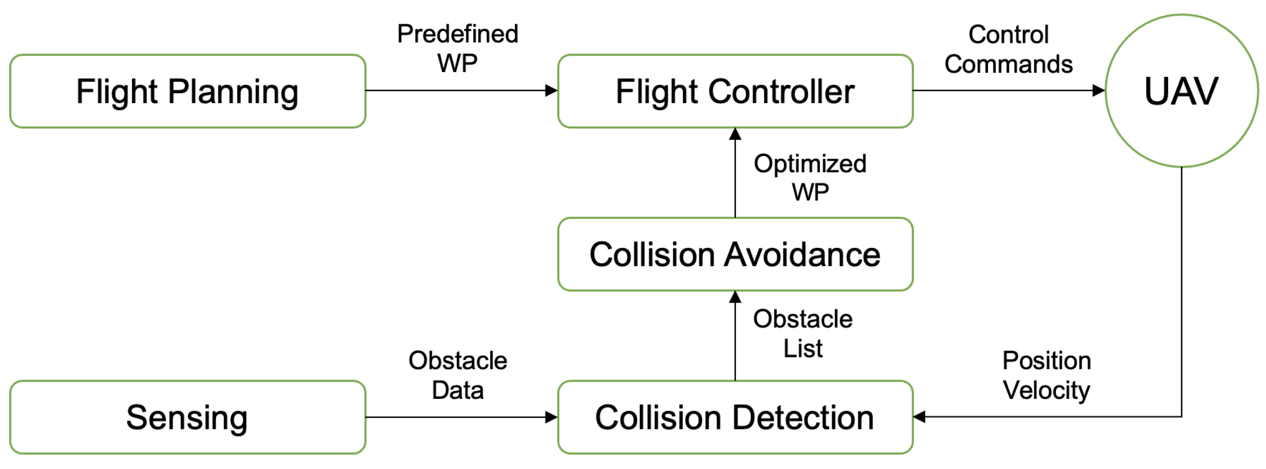
This work aims to address parts of a comprehensive obstacle detection and collision avoidance system, thereby representing a two-stage “sense” and “avoid” problem. The generic Sense and Avoidance (S&A) system architecture is depicted in
Figure 1. Notice that the outcome of the system is to feed updated flight trajectory information to the flight controller, such that the UAV can continue to navigate safely. This all starts with the sensing system, so its definition and performance are critical.
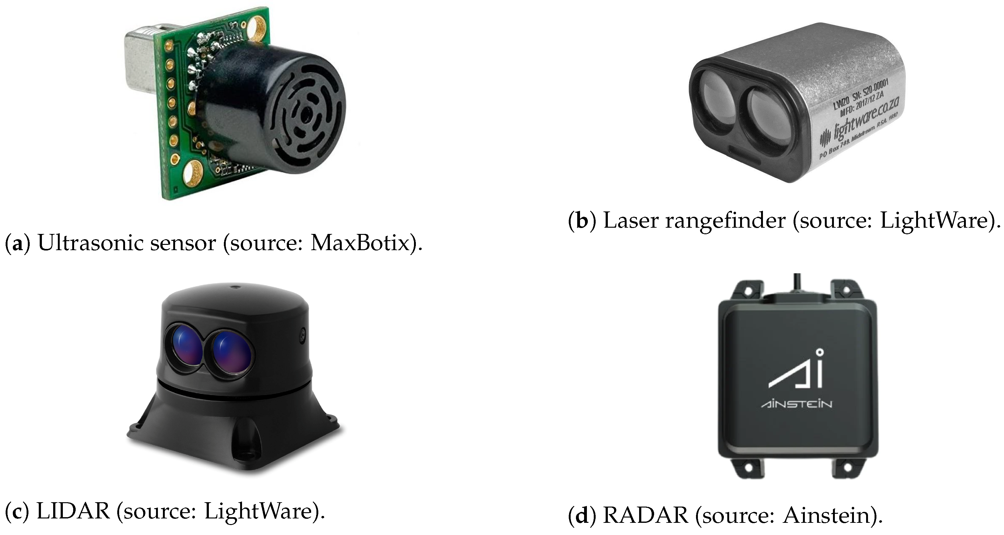
In this study, the sensors used to gather obstacle data are the ultrasonic sensor, laser rangefinder, Light Detection and Ranging (LIDAR) sensor, and Radio Detection and Ranging (RADAR) sensor.
Ultrasonic sensors generate sound waves, which are then reflected by the obstacle and recorded by the sensor. In knowing the speed of the radiated sound in the air medium, the distance from the point of greatest reflection to the obstacle can be calculated. Using these sensors proves to be advantageous mainly due to the ease at which this simple technology can be sized down, which is why ultrasonic-based systems were proposed for a similar application [
8]. However, because these are proximity sensors, their signal quickly attenuates and their capacity to measure distance is typically limited to less than 10 m [
9].
Laser rangefinders are able to compute the distances to obstacles by emitting a laser pulse and measuring the time it takes for the reflected beam to be detected (given that laser light beams move at a known speed). This principle is quite common among sensors, and it accounts for lightweight, low-cost technology [
10]. However, it is limited by weather conditions, as laser light might scatter in the presence of clouds, fog, or atmospheric attenuation.
The Light Detection and Ranging (LIDAR) working principle is similar to the laser rangefinder, except it is multi-directional thanks to an oscillatory base; thus, its execution goes beyond simply detecting an obstacle’s range, and a 2-D point cloud can be acquired through a vast array of distance and azimuthal measurements pairs. LIDARs installed on UAVs can accurately delineate the shapes of objects at fair distances, (more than 30 m), as demonstrated on a LIDAR-based system for tree measurements [
11], thus making them main candidates to incorporate an obstacle detection system.
Radio Detection and Ranging (RADAR) is one of the most popular sensing technologies. It consists of a transmitting antenna that produces electromagnetic waves (in the radio or microwave spectrum) and a receiving antenna, which collects waves echoed from static or dynamic obstacles [
12]. Despite being very similar to LIDAR, RADAR technology is distinguished by the frequency of the emitted radiation. The distance between the sensor and the target is also computed by measuring the time lapse between the transmitted and received signal since radio waves also move at a known speed.
Vision technology can acquire richer information from surroundings, involving color and texture, while being cheaper and easier to deploy in comparison to the aforementioned sensors [
13]. However, image sensors face challenges in achieving high accuracy due to their dependency on texture, lighting, and weather conditions. Furthermore, all cameras rely on real-time heavy image processing to extract useful information from the chunks of raw data being provided by the sensor [
14], thereby greatly increasing the computational complexity of this application. Therefore, vision-based sensors were deemed unsuitable for the present study.
It is important to note that most research in this field focuses on multirotor UAVs. Among these, solutions typically include cameras [
15], LIDAR technology [
16], or both [
17]. That was not the case for the solution presented in [
18], where the solution was specifically designed to map indoor spaces with planar structures through graph optimization. Using many 1D lasers to maximize the orientations that are being covered, as opposed to using a single 2-D LIDAR, allows for a more accurate hypothesis of the planar structures—one that is free of assumptions about the horizontal and vertical planes. Furthermore, the viability of an acoustic-based collision avoidance system for a fixed-wing UAV that resorts to microphone data as the main input was also investigated with limited success [
19].
Regarding flight planning and collision avoidance, a recent work aimed at implementing UAV path re-planning and evasion maneuvers through deep reinforcement learning [
20]. A deep reinforcement learning approach for three-dimensional path planning by using local information and relative distance without global information, i.e., resorting to a partially observable Markov decision process, was proposed [
21]. In contrast, the present solution focuses primarily on the detection capacity of different sensors and how to optimize their resources, thus resorting to a simpler Potential Fields collision avoidance method.
Preceding this work, different detection systems were simulated using laser rangefinders and RADARs in different configurations [
22]. Through the Potential Fields method and resorting to an optimization algorithm, a possible configuration of a UAV detection system was reached. Subsequently, ultrasonic sensors and laser rangefinders have been employed in the hardware implementation of an effective sense and avoid system on a simple rover [
23].
The main goals are to (1) perform a comprehensive study of the four main, active non-cooperative sensor types (ultrasonic sensor, laser rangefinder, RADAR, and LIDAR); (2) develop models for each type and embed them in an obstacle detection and avoidance simulation tool; and (3) perform off-line simulations using randomly generated collision scenarios to obtain optimal multi-sensor configurations in terms of sensor types, positions, and orientations that maximize the obstacle sense and avoidance success rate for a given set of performance parameters of a small fixed-wing UAV.
The current work is limited to 2-D problems, and it is assumed that the UAV is in level flight (constant altitude) at cruise conditions and remains so during the obstacle detection and avoidance stages. For fixed-wing aircraft, this might represent the vast majority of its flight.
2. Sensor Modeling
The next subsections describe the models of active non-cooperative sensors: the ultrasonic sensor, the laser rangefinder, the LIDAR (Light Detection and Ranging) sensor, and the RADAR (Radio Detection and Ranging) sensor. These are illustrated in
Figure 2, and are followed by a comparative analysis, as shown in
Table 1. Certain models were developed by [
24] and are further adapted to the present work.
The relevant sensor specifications are summarized in
Table 1. Although the obstacle detection capability depends greatly on the range, field-of-view (FOV), accuracy, and update rate of the sensors, other aspects should also be taken into account during the selection of parts. The size and weight of sensors are crucial factors to consider when designing a S&A system for small UAVs since it may be counterproductive to add detection capability at the cost of reduced vehicle maneuverability. This is likely not the case for the particular set of sensors in this study, with the MB1242 sonar being the smallest and lightest; followed by the slightly larger and heavier LW20/C laser; then the SF45/B LIDAR that is almost double in size; and the US-D1 RADAR, which—while the largest and heaviest—is still sufficiently compact for application in small UAVs. Power consumption can be particularly important since most UAVs are battery powered; thus, LIDAR and RADAR are at a clear disadvantage compared to the ultrasonic sensor. Regarding acquisition cost, the ultrasonic sensor is the cheapest sensor, while the laser-based and RADAR sensors are considerably more expensive. Unexpectedly, the SF45/B LIDAR with a variable FOV is more costly than the LW20/C one-dimensional laser rangefinder, and the US-D1 RADAR is the most expensive at twice the cost of the laser due to its pricier technology.
2.1. Ultrasonic Sensor
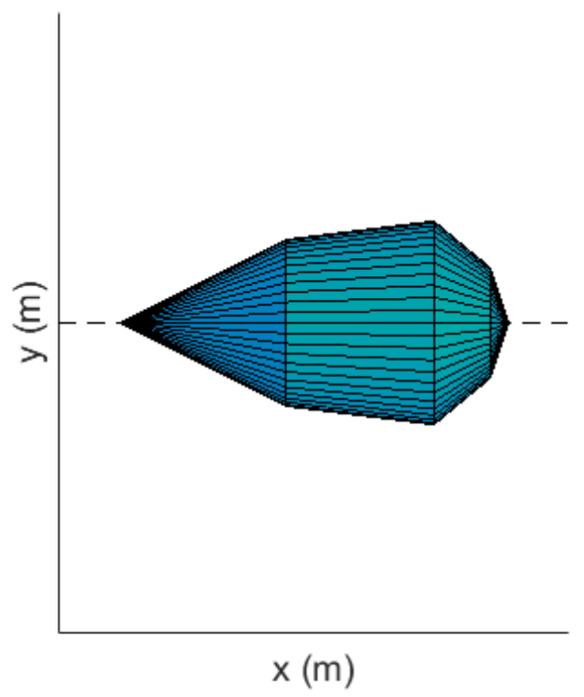
This type of sensor has a wide FOV that translates to a beam pattern with axial symmetry, as represented in
Figure 3.
Since the ultrasonic sensor only outputs a distance, it leaves all the interior beam points located at a specific distance from the UAV as potential object positions. This results in errors that can be avoided, as well as other issues that arise from sound reflection. The sound reflection law states that the reflected sound wave’s angle with the normal of the surface is preserved. Thus, the ultrasonic sensor requires a perpendicular surface in order to detect an object, which, in turn, implies that the targets format is crucial to the mission’s success. It is vital to recognize that the final results can only be used as a reference given that these simulations only use spherical shape targets (and different target formats could either improve or worsen the outcome). In short, the model must check for the following possibilities at all times:
Verifying these conditions requires considerable computing time. Therefore, a progressively complex approach was implemented [
23]. First, the beam pattern is reduced to a cylinder. When the center of the obstacle is found to be inside the cylinder, a more thorough analysis is performed to identify which portion of the spherical surface, if any, is in fact inside the beam pattern. The last stage addresses the perpendicularity issue. The final surface computed in the preceding phase is defined as a list of points. The aim is to calculate the angle between the direction of the sound wave and the tangent surface of the sphere at that precise location. The point is deemed to have been picked up by the sonar if the angle is close to 180
(with a 5
tolerance). Although the vast majority of the final surface points were inside the beam pattern, all of the points that were designated as detectable required a second examination. The closest point to the UAV position (among those that passed these filters) was chosen as the detected point. The UAV reference point, which will serve as the reflection point for the trajectory re-planning algorithm, will be situated on the beam pattern axis at the same distance from the UAV as the detected point.
2.2. Laser Rangefinder
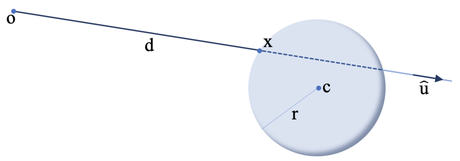
Considering the obstacles as spheres, the reflection point can be modeled as a simple interception between a line and a spherical surface in
Figure 4, which is given by
where
is the detection point on the line and/or sphere,
is the center point of the sphere,
r is its radius,
is the unit vector that defines the line direction in
space, and
d is the distance from the origin of the line
. Combining both equations leads to an easily solvable quadratic equation,
which returns a solution
d if
, where
is the sensor detection range. In real conditions, the laser would not reach the furthest point, it would instead reflect on the closest one. Therefore, if there are two solutions in this interval, only the smallest one prevails. The reflection point with a spherical surface can be easily obtained from Equation (
2).
2.3. LIDAR
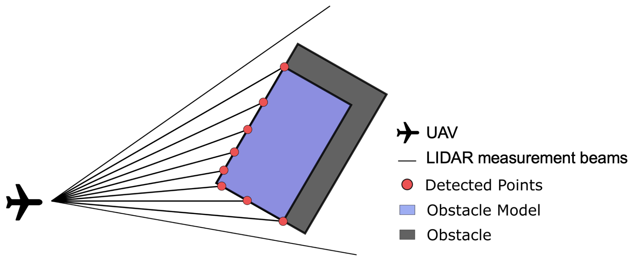
This type of sensor is not limited to a distance output as it can also provide the system with an azimuthal angle where the distance was measured, i.e., the LIDAR model has to account for outputs with polar coordinates. The LIDAR model is very similar to the laser rangefinder’s, in which it makes only the points that are closest to the sensor detectable. This implies that if an object is completely visible, then only half is detected, and the remaining half of the obstacle is reconstructed via symmetry, where the center of symmetry is the medium point of the segment connecting the first and last point of the cluster. In the present simulations, this distance corresponds to the diameter of the obstacle. The symmetry assumption brings no drawbacks since the LIDAR is continuously scanning and updating the detected points, thus providing an up-to-date front-facing geometry of the obstacle. The model discards obstacles that are hidden or outside the field of view (FOV).
A common issue lies within higher distances between consecutive points in farther obstacles, which results in smaller detected dimensions (compare Obstacle and Obstacle Model in
Figure 5). To solve this problem, the measured diameter is passed through the time filter, as proposed in [
29],
where
is the filter gain,
is the filtered diameter at instant
is the filtered diameter at instant
, and
is the measured dimension at instant
. The gain must be carefully chosen because it affects how quickly the dimensions change. While a small gain (i.e., a slow variation) is better for noisy surroundings, it is not appropriate for objects with high relative speeds. The gain is given by
where
p corresponds to a fraction that represents the desired accuracy of the dimensions and
n corresponds to the number of filter cycles required to get an accuracy of
p. Classic Kalman filters [
30] were employed for the tracking phase, where the motion of obstacles was assumed to be two-dimensional, linear, and constant over successive scans. This simplification, which takes into account a high scanning frequency, accurately captures the targets’ state.
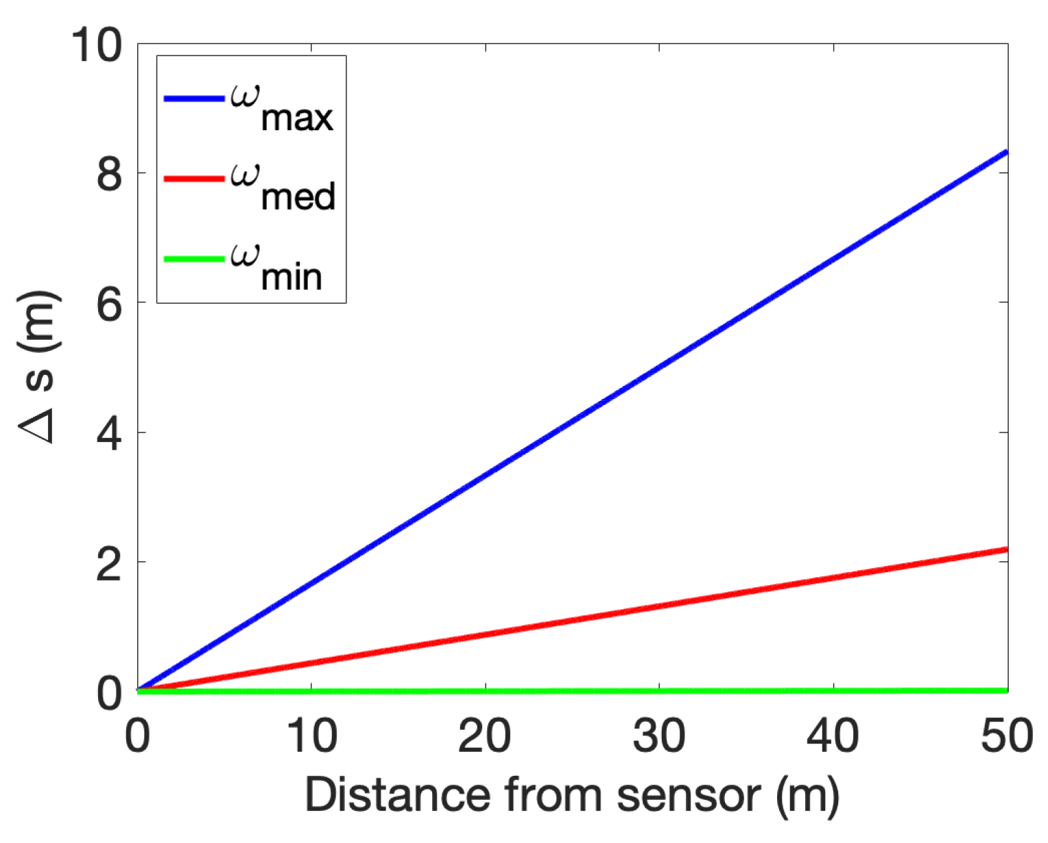
The LIDAR model in use (based on the LightWare’s SF45/B) has a specific update rate, but it is possible to set its angular velocity (scanning speed) up to a maximum of 6.3 rad/s. However, by choosing faster sweep speeds, the arc of circle that is not being detected between each measurement increases, thus increasing the likelihood of missing an obstacle smaller than that arc. This effect is illustrated in
Figure 6, where the length of the arc traversed
varies analytically with the distance to the sensor and the angular velocity. At maximum scanning speed (
), this 45 m range LIDAR might not detect obstacles that are smaller than 8 m wide at this distance. However, if covering a larger area quickly is more important, sacrificing some visibility at the maximum range might be acceptable. Ultimately, the compromise should be based on the specific needs and constraints of the system.
2.4. RADAR
In this case, the state estimation is more complex than the one employed in the LIDAR model (given the RADAR sensor provides the distance, azimuth, and elevation of the observed obstacles). These outputs are spherical, but only the polar components (distance and azimuth) are considered in the 2-D model. Since the intruder dynamics are best described in rectangular coordinates, the converted measurement Kalman filter (CMKF) was used to convert the measurement data in polar coordinates into a Cartesian coordinate system, so that the tracking could be realized through a linear Kalman filter [
31]. The 2-D model used in the simulations was then represented by
where
are the measurements converted to the Cartesian frame,
is the measured range,
is the measured azimuth, and
is the bias compensation factor expressed as
where
is the standard deviation of the noise in the azimuth measurements. The compensation of the bias is multiplicative due to the use of the unbiased conversion and modeling the measurement errors as Gaussian white noise. The covariance matrix used in the Kalman Filter is given by
with the details of the computation of these variances found in [
32].
2.5. Multi-Sensor Data Fusion
All of these sensors (and respective models) provide inputs that allow the avoidance system to actuate. However, if the system’s architecture is composed by more than one sensor, the data provided must be merged in some way. The sensor models previously described provide the required mutual transformation of their measurements into one global Cartesian coordinate system. Also, synchronization is guaranteed by the time schedule used for retrieving the obstacle sensing data from models.
Following the best practices proposed in a similar application [
33], the weighted filter method was used in the present study for data fusion. The principle behind this method is simple: each sensor is given a weight that is based on how reliable it is. Reference data sensors that provide information about the UAV state must be installed. Considering that changes in the distance to obstacles correspond to changes in the UAV location, reference data sensors like IMUs and optical flow sensors are used to assess the accuracy of the main data and aid in selecting the best sensor. In the particular case of fixed obstacles, the aforementioned variances in distance ought to match. The weights are then calculated by applying a differential norm to compare all of the conceivable sensor combinations of the main data and reference data. In each instant, the obstacle distance measurement corresponding to the sensor with the lowest weight is chosen, and the remaining measurements are discarded on the grounds that they are corrupted. Nonetheless, the sensor readings are fused in accordance with their weights if the computed weights have a low variation.
4. Optimal Sensing System
An optimization study was conducted to find the types of sensors and respective orientations relative to the UAV longitudinal axis that result in the best collision avoidance performance. To do so, a set of randomly generated collision scenarios with both fixed and moving obstacles were generated. The sensors modeled in
Section 2 were tested for each of these scenarios, and their orientations were varied until optimal configurations were found.
4.1. Scenario Generation
To create scenarios suitable for this study, a scenario generation algorithm was used, in which the predetermined path and waypoints of the UAV as an input was accepted before combining them with a list of moving and static obstacles to produce a scenario [
23]. Each scenario must specify the obstacle’s initial position, velocity, and radius. It should also include a pre-planned path and waypoints that the UAV must follow.
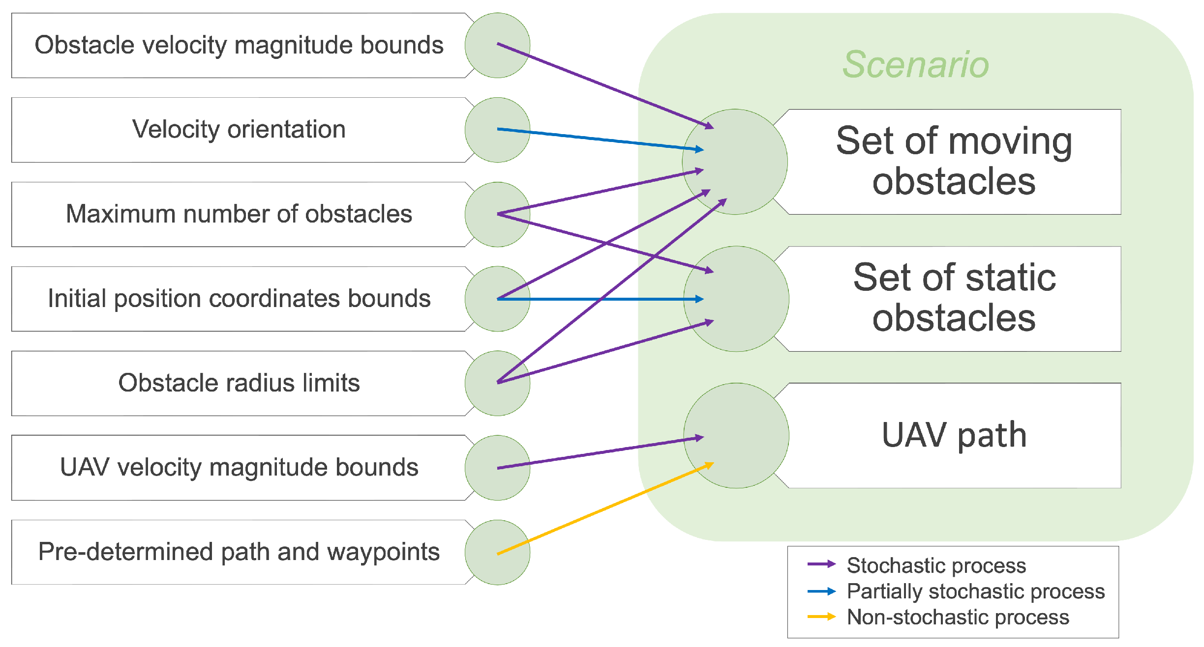
Different bounds were defined regarding the kinematic and dimensional properties of the obstacles and the UAV itself. Various stochastic and partially stochastic processes were then extracted from these intervals, creating random values for the different variables, as depicted in
Figure 10. Partially stochastic processes were used in two different cases: determining the velocity orientation of moving obstacles and setting the position of static obstacles. In the former, the goal was to ensure that, initially, the direction of the obstacle’s velocity should point to the center of the domain rather than pointing outward, thus increasing the possibility of collision. In the latter, the position of any static obstacle must not be within a determined safety radius around the waypoint given that the UAV must pass through it. All remaining bounds but one were used to select a completely random value that ultimately defined each set of obstacles. In addition, a pre-determined flight path was loaded, which accounted for a non-stochastic process, into each scenario.
Finally, each scenario was tested for potential collisions using a flight simulator without any sensors (with the obstacle avoidance strategy turned off). This was then discarded if the UAV did not go beyond any obstacle’s safety radius throughout the whole flight simulation. This function was repeated until n scenarios with an impending collision were generated.
In this study, forty collision-leading scenarios were randomly generated, with obstacle parameters varying according to the limits set in
Table 2 for the UAV speed, number, and size of fixed and moving obstacles, as well the velocity of the latter. The UAV speed and maneuvering capabilities were based on the Tekever AR4 small fixed-wing model, in which a maximum turning rate of 45
/s [
36] was assumed.
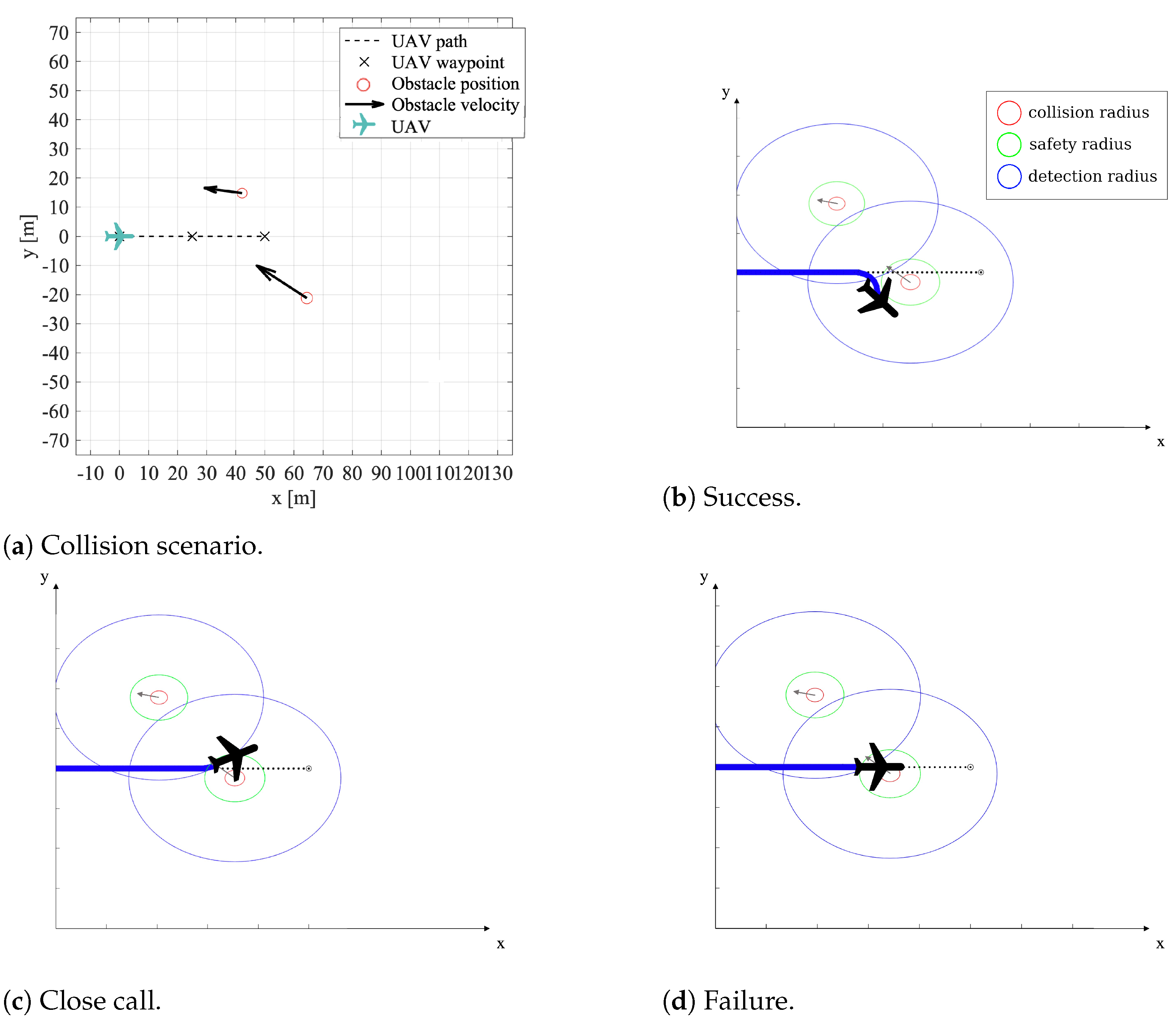
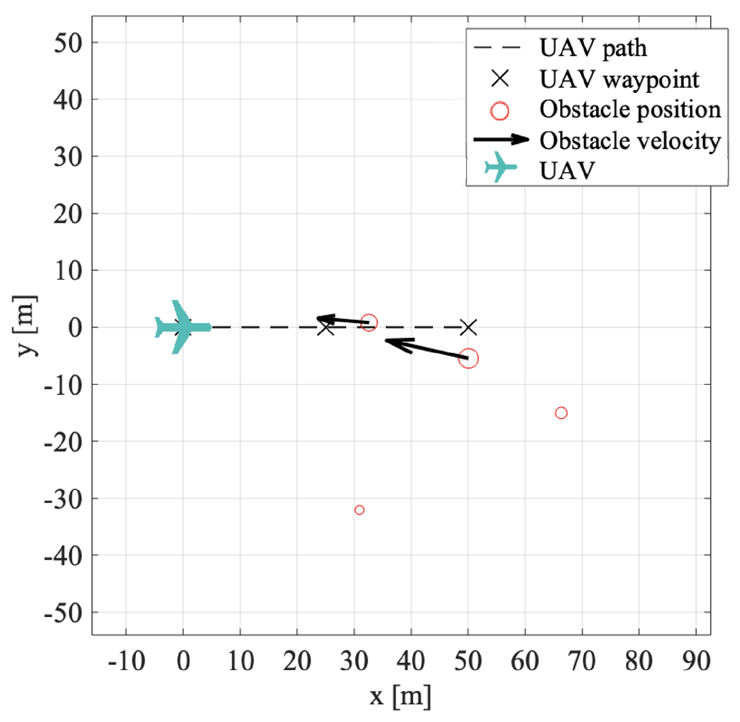
An example of a resulting collision scenario is plotted in
Figure 11, where two moving obstacles in a collision course with the planned UAV flight path can be observed.
4.2. Optimization Technique and Problem Formulation
To determine the optimal sensor configuration, different sensor sets were tested. The parameters that characterize each sensor model were obtained from their technical manuals or inferred from the available data summarized in
Table 1. Since our simulations were restricted to the horizontal plane of motion, the vertical FOV was not relevant.
Given that all sensors may be mounted at an angle relative to the UAV longitudinal axis, our model assumed the use of two symmetrical sensors at the angles and whenever .
In order to optimize the sensor orientation
, a Sense and Avoidance (S&A) metric function
was minimized and defined as
where the first term drives the evasion maneuver to maximize the minimum distance
between the UAV and the obstacle
i, the second term represents the penalty when the minimum distance violates the safety radius
, and the last term represents the penalty when the minimum distance violates the obstacle collision radius
. The metric accumulates not only for every obstacle
i in each scenario, but also for all scenarios
j. In order to penalize collision cases more than close calls, the weights were set to
and
. Notice that the sensor orientation
was kept fixed during the simulations with the 40 scenarios, and it was only considered variable when determining the best installation orientation of the sensor attached to the aircraft (Equation (
12)).
The deceptive look of the metric function defined in Equation (
11), might suggest that least-squares or quadratic programming methods would be adequate. However, the metric is far from satisfying the required properties since the terms
vary in a highly non-linear fashion with variable
.
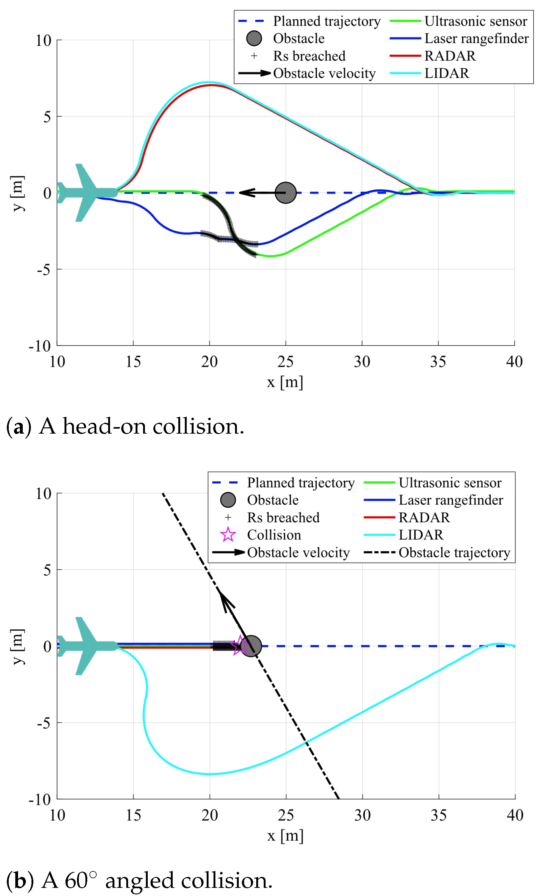
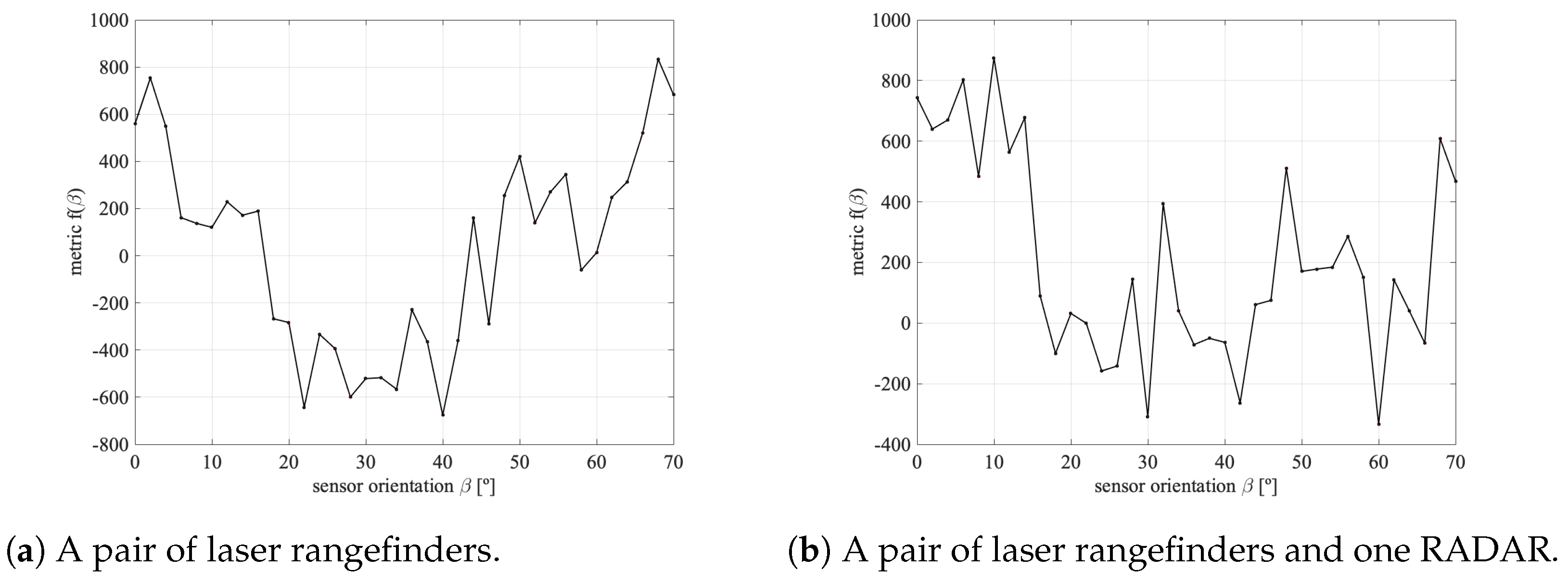
Figure 12 shows the metric function value defined in Equation (
11) for two particular sensor sets: (i) using only a pair of laser rangefinders with a 100 m range that symmetrically pointing forward with an angle
with respect to the UAV longitudinal axis; and (ii) adding a RADAR with a 120 m range pointing in the direction of the UAV longitudinal axis. In both cases, the metric function
proved to be multimodal and noisy.
These identified metric function properties conditioned the choice of the optimizer. Gradient-based optimization methods were discarded since they would struggle in the presence of noise and would become stuck in local minima. Among the vast choice of gradient-free (or derivative-free) methods available in the literature [
37], in particular those that find near-global solutions for non-convex problems, the Genetic Algorithm (GA) implemented in MATLAB was selected in this work. While there are other newer and better performing methods, its ease of implementation prevailed when making the choice. Its higher computational cost is acceptable since its usage occurs in the design stage of the obstacle detection system, i.e., prior to the installation of the sensors and pre-flight. The stochastic nature of GA, as it involves crossover (exploitation) and mutation (exploration) operators over a population of solutions, allows for it to explore a broader solution space and adapt to the challenges posed by noise and multimodality, as well as allows for it to handle the uncertainty introduced by noisy objective functions more effectively. Additionally, the exploration–exploitation balance in the GA enables it to navigate multimodal landscapes by maintaining a diverse population and evolving solutions over generations (iterations).
The problem can be posed as a non-linear-bound-constrained optimization,
where
and
are the lower and upper bounds of
, respectively, to be defined for each particular case. Notice that
is a vector if multiple sensors are used.
The initial GA population was set to be created with a uniform distribution. The crossover function was set to create of the population in each generation. Moreover, because the variables were bounded, the mutation function randomly generated directions that were adaptive with respect to the last successful or unsuccessful generation, where the chosen direction and step length satisfied the set bounds. The convergence criteria were set such that the global minimum was found in a timely but accurate manner: a function convergence of was used with 10 stall generations, and a maximum of 50 generations were prescribed. The population size was set to 30 individuals. These parameters were chosen following best practices. Larger populations and stricter convergence criteria were also tested but led to no significant impact on the results presented. The simulations were run on an 1.4 GHz Intel quad-core i5 with 8 GB 2133 MHz RAM.
4.3. Optimal Sensing Configurations
The following subsections are dedicated to detailing the proposed sensing architectures, in which further explanations of each solution and the respective optimal results are detailed. In the end, the performance of the different sensor sets are summarized and compared in order to implement the best solutions.
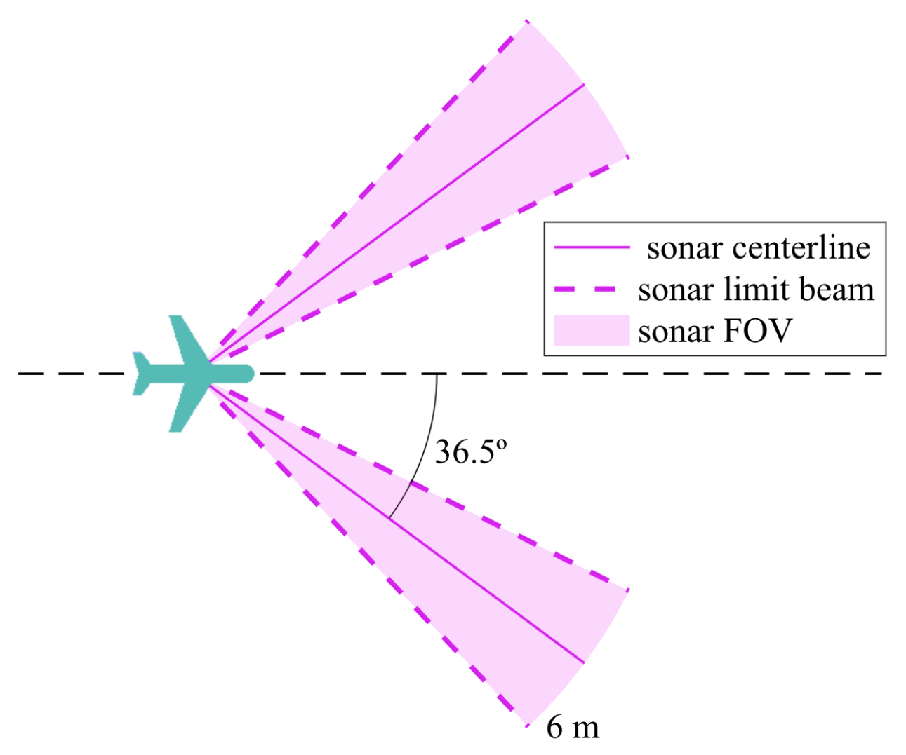
4.3.1. Two Ultrasonic Sensors
For a set of two ultrasonic sensors, the orientation of each sensor was bounded between and from the longitudinal axis, and the range was set to 6 m. To simplify the problem, the two sonars were considered to have a symmetrical orientation, resulting in just one design variable. A narrow beam pattern was adopted to reduce computational cost.
The GA minimization terminated after 20 iterations due to average changes in the fitness value being less than the specified tolerance. It performed 592 function evaluations in 18 h and 36 min, and it reached an optimal orientation of
(see
Figure 13).
The results, summarized in the second line of
Table 3, were far from satisfactory since the safety radius was breached many times, thus leading to a collision rate of 10 %. Compared to a single sonar pointing forward (see first line in
Table 3), a pair of sonars brought little to no gains in the detection performance for the type of UAV under study. This was expected due to the short range of ultrasonic sensors, which makes it impossible for the UAV to detect the obstacle, re-plan its trajectory, and perform the avoidance maneuver in a timely manner.
When considering a UAV traveling at maximum speed (15 m/s), the ultrasonic range (6 m) was traversed in 0.4 s. In the worst case with an obstacle moving at 15 m/s head on, the available reaction time of just 0.2 s was clearly insufficient.
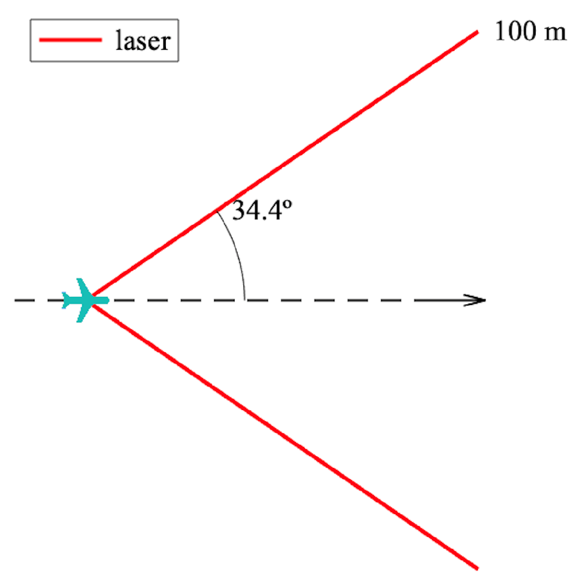
4.3.2. Two Laser Rangefinders
Analogous to the previous case, a set of two laser rangefinders with symmetrical orientations but with a sensing range of 100 m was considered.
After 19 generations, the GA optimization algorithm finished having completed 564 function evaluations in a computing time of 1 h 25 min. The optimal sensor orientation was
, which corresponds well with one of the approximate minimums shown in the preliminary study, as shown in
Figure 12. The optimal two laser rangefinder sensor configuration is illustrated
Figure 14.
The performance of this optimal configuration is summarized in the fourth line of
Table 3. Although the optimal configuration only failed once in 40 scenarios, the safety radius was breached in 23 of them. This result was expected since a UAV equipped only with two laser rangefinders (with extremely narrow FOVs) is not capable of properly tracking moving obstacles when collisions are imminent. Also, there were gains when using more than one laser (see third line of
Table 3), which made up for the reduced, almost zero, individual FOVs.
Compared to the previous case of ultrasonic sensors, these simulations demonstrated that laser rangefinders not only prevent more collisions, but also more close calls. This is mainly a consequence of their large detection range advantage (100 m), which prevail over their almost zero FOV. Overall, these sensors perform better under the given circumstances.
When considering a UAV traveling at 15 m/s, the laser range was traversed in 6.7 s. If an obstacle was also moving at 15 m/s head on, the available reaction time was 3.3 s, so it was typically enough to track an obstacle and re-route, provided it was tracked because of a reduced FOV.
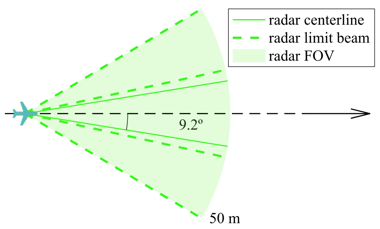
4.3.3. Two RADARs
Once again, the two RADAR sensors were considered to be symmetrical on the UAV longitudinal axis and the orientation spanned from to . Each RADAR had a range of 50 m, an accuracy of 0.04 m, and a FOV of .
After 11 generations, the optimizer finished 340 function evaluations and a computing time of 1 h 11 min. The optimal RADAR orientation was
, as illustrated in
Figure 15.
Another configuration worth studying would be a sensor orientation that is close to
, which would yield the same result as if the UAV were equipped with a single RADAR with a double FOV (
).
Table 3 includes a comparison of a single RADAR pointing forward and a solution with two RADARs in the seventh to eighth lines.
Regarding actual collisions, obstacles that approach the UAV from an angle are more likely to be detected by the optimal solution rather than by the single-RADAR configuration. As can be seen in
Table 3, the number of failures increased as the orientation decreased (for this particular case), which in turn made the success rate decrease.
By overlapping the FOV of the two sensors, the accuracy was reduced through the data fusion algorithm. Thus, in this case, having a narrower FOV () and, in turn, the juxtaposition of both RADARs proved to be almost as effective as the double FOV configuration ().
These simulations showed that the accuracy of RADAR proved to be impactful on the precision of obstacle tracking compared to that of the laser sensors. The latter’s accuracy can not be reduced through the data fusion algorithm since a laser FOV would not overlap (). Despite having a broader FOV and resulting in less close calls, the RADAR solution led to just as many collisions, which means that the two-laser rangefinder configuration displayed the same success rate. It is reasonable to say that, while RADAR FOVs are more crucial for detecting obstacles, the sensor’s accuracy is the most significant factor for effective collision avoidance.
When considering a UAV traveling at 15 m/s, the RADAR range (50 m) was traversed in 3.3 s. If an obstacle was moving at 15 m/s head on, the available reaction time was 1.7 s, which might be a challenging time to successfully complete an evasion maneuver. However, the tracking is likely to be more successful given the large FOV.
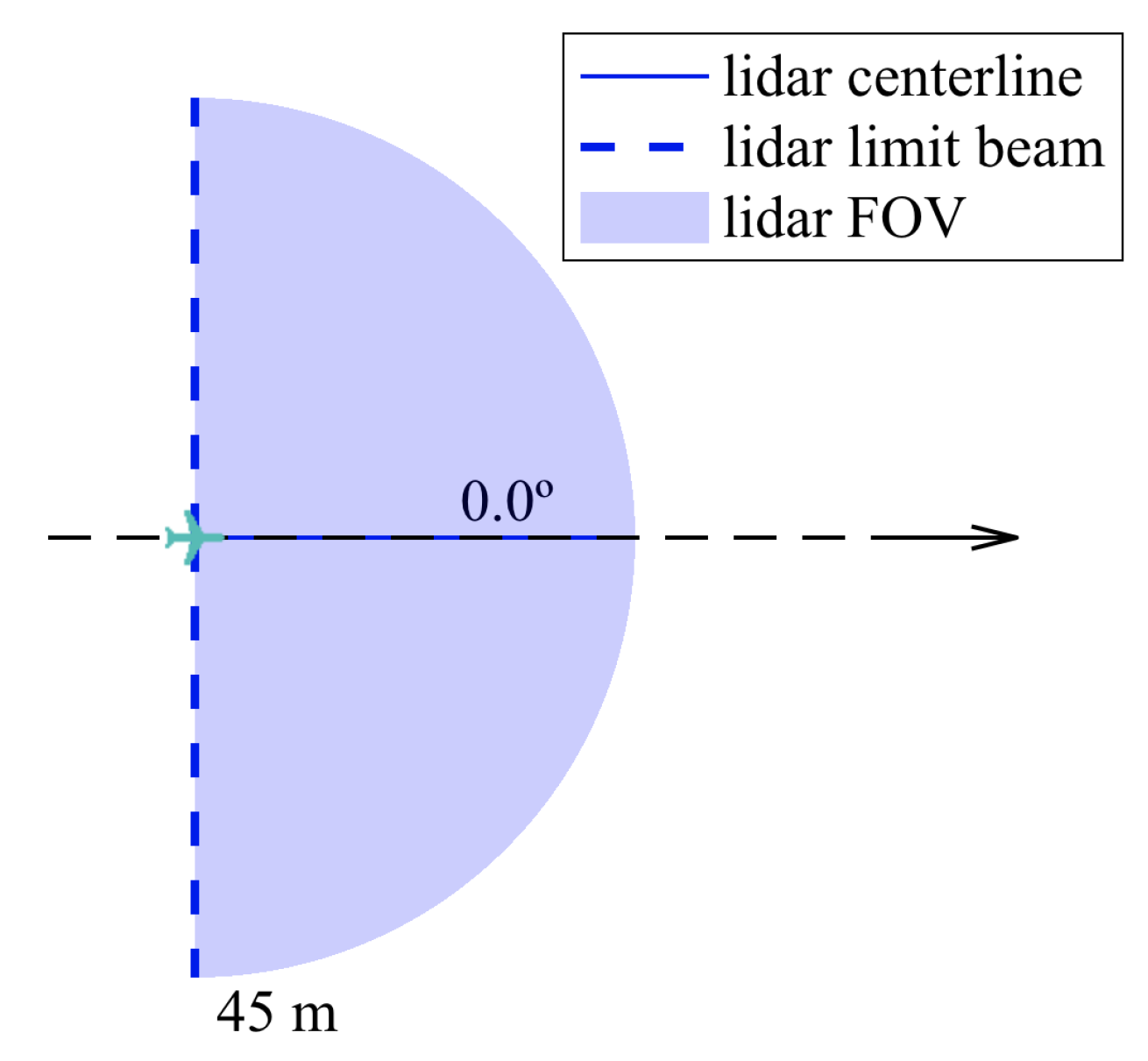
4.3.4. Two LIDARs
Each LIDAR was modeled with a range of 45 m, an accuracy of 0.1 m, and a variable FOV. According to hardware specifications (see
Table 1), this FOV can range from
to
; thus, a FOV of
was chosen. This value ensures a reasonable trade-off between timely scanning frequency and a broad scope.
However, this makes optimization redundant due to the nature of the scenario generation algorithm used: because the obstacles spawn inside the limits of the scenario, it is worthless to track the area behind the UAV in the initial instant. Furthermore, from this instant on, if an obstacle was positioned behind the UAV, it would have already been tracked before due to the wide FOV and long range of the LIDAR. The overlapping of the FOV in the case of a two-LIDAR solution did not prove to be advantageous either. (Note that this was only verified for a FOV of
). The problem would only arise if a narrow FOV was set due to measurement speed considerations (see
Section 2.3). For a smaller FOV, it would be convenient to optimize the sensor orientation.
In this particular case, it is fair to state that the most beneficial solution would be to use a single LIDAR pointing forward since it decreases hardware cost. This configuration is illustrated in
Figure 16.
The last line of
Table 3 includes the performance of the single-LIDAR configuration. Compared to the previous types of sensors studied, the LIDAR performed better overall. The reasonable detection range and the wide FOV reduces the chances of close calls and eliminates the possibility of failure.
When considering a UAV traveling at 15 m/s, the LIDAR range (45 m) was traversed in 3 s. If an obstacle is moving at 15 m/s head on, the available reaction time is 1.5 s, so a similar obstacle detection and avoidance performance to the RADAR is expected.
4.4. Performance Comparison of Sensor Sets
Other solutions that involved three sensors were optimized; for example, two laser rangefinders that were symmetrical about the UAV longitudinal axis and whose orientations were bonded between
and
, and one fixed RADAR pointing forward. This configuration was also replicated with two lasers and one LIDAR; two RADARs and one laser; and two RADARs and one LIDAR. The performance of the optimal version of these sets of sensors, as well as the results from the solutions with only one type of sensor that are discussed in the previous subsections, is summarized in
Table 3. Optimizations with different sets of sensors were performed but left out of this table in order to avoid redundancy in the results.
As seen before, for the set of scenarios tested, RADAR performed better than the laser rangefinder, which, in turn, performed better than the ultrasonic sensor if only one sensor type was to be used. Nonetheless, this is tightly dependent on the sensor characteristics, such as range, FOV, and accuracy. Furthermore, a single LIDAR was enough to outperform all other types of sensors.
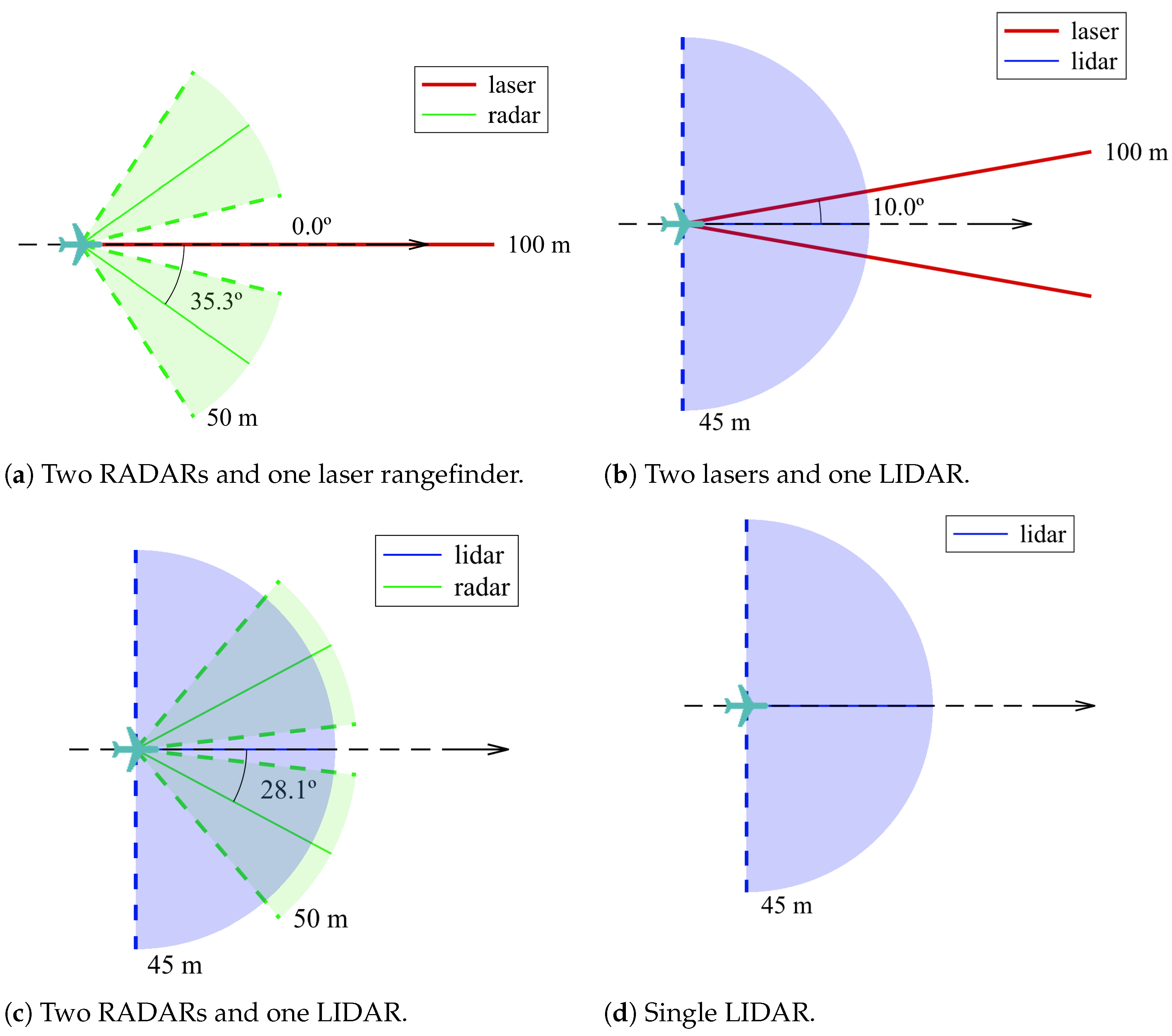
As expected, all the solutions that present a 100% success rate include either a RADAR or a LIDAR in their configuration, thus attesting the importance of sensor range and FOV for a timely trigger of the avoidance maneuver. If the LIDAR is kept out, it is the two-RADAR and one-laser rangefinder solution represented in
Figure 17a that produced the least collisions and led to the least close calls. From these findings, and because of the
FOV of a laser rangefinder, it is expected that increasing the number of sensors even more would lead to an even better performance, though at a higher hardware cost.
When comparing the solutions that include a LIDAR, it was proved that it is not significantly advantageous to pair it with other types of sensors since it already performs distinctively well on its own. The single-LIDAR solution, as shown in
Figure 17d, exhibited a 100% success rate. This meant that no collisions were registered due to its wide FOV and considerable range, thus making it able to detect obstacles before they become a threat without the aid of additional sensors. Regardless, the two-laser (
Figure 17b) and the two-RADAR (
Figure 17c) solutions were beneficial for also reducing the likelihood of close calls. Despite the LIDAR configuration having a wide FOV that was not increased by either configuration, the chances of breaching the safety radius decreased because the other sensors provided additional detection capacity, i.e., since the LIDAR swept the designated area at a certain frequency, there were time instants when a fraction of the area within the LIDAR FOV was ’unsupervised’. Therefore, it is useful to have another set of sensors that track obstacles approaching from that specific area.
To summarize, the optimized configuration had a very similar performance in four different cases (reflected in the Metric column). The most promising one (with the smallest metric value) was composed of one LIDAR pointing forward complemented by two laser rangefinders pointing at 10
sideways. That was the only configuration that resulted in only 8 close calls out of 40 maneuvers. The other three configurations, also with which no collisions registered, resulted in 9 close calls. It is also interesting to note that, in the configurations listed in the last three lines of
Table 3—despite having the exact values for failure, close call, and success rate—the metric function value varied. Recalling that not only does the metric function penalize breaching the safety and collision radii, but also accounts for the maximization of the minimum distance between the UAV and obstacles (see Equation (
11)), then the lowest metric value of the two-RADAR and one-LIDAR solution reflected its ability to maintain a greater distance to the surrounding obstacles among these three configurations.
5. Conclusions
This work presents a comprehensive solution for enhancing the safety of small fixed-wing UAVs by addressing the critical issue of obstacle detection during flight. A set of select sensors, namely the ultrasonic sensor, laser rangefinder, LIDAR, and RADAR, were identified and further employed in modeling collision detection and avoidance simulations using the Potential Fields method.
To determine the best combination of sensors and their orientations, these simulations were used in an optimization study. The study revealed that relatively simple detection configurations can yield a high success rate in collision avoidance. While the ultrasonic sensor was found to be inadequate due to its limited range, the laser rangefinder benefited from a long range but had a restricted FOV. On the other hand, both the LIDAR and RADAR configurations proved to be the most promising options, offering not only a substantial range, but also a wide FOV. Based on the optimization study, the recommended multi-sensor configurations consist of a front-facing LIDAR accompanied by either two laser rangefinders pointing sideways at or two RADARs at .
The two most promising solutions included a LIDAR, so it is important to note that the practical implementation of this type of sensor brings forth a set of challenges that must be carefully navigated for optimal performance in real-world scenarios. Cost is a critical factor influencing the feasibility of LIDAR-based obstacle detection systems. While LIDAR technology has advanced rapidly, the associated costs can be prohibitive, especially for smaller UAVs with limited budgets, so striking a balance between affordability and performance is crucial to ensure the widespread adoption of obstacle detection systems. Also, the compromise between sweep angle and speed is a nuanced consideration in optimizing collision avoidance systems since a wider sweep angle with faster sweeping speeds enhances coverage at the expense of possible missed detections, thus limiting the system’s ability to identify threats.
While the particular solutions found here are strictly valid for the set of UAV flight performance parameters used, this work provides a generic comprehensive methodology for determining an optimized multi-sensor system configuration that holds great potential for enhancing the safety of small fixed-wing UAVs in flight.
Future work is twofold. Firstly, the extension to 3-D problems, both in terms of obstacle detection and collision avoidance maneuvers, adds an additional degree-of-freedom to the sensors’ optimal orientation and elevation angle, as well as allows for climb and descent maneuvers. Lastly, the validation of the proposed multi-sensor system configurations implies challenging hardware and flight controller software implementations for flight testing. The collision avoidance method is then meant to run real time on board, and it is fed by live distance sensor data.


