Autoignition Problem in Homogeneous Combustion Systems: GQL versus QSSA Combined with DRG

Abstract

The global quasi-linearization (GQL) is used as a method to study and to reduce the complexity of mathematical models of mechanisms of chemical kinetics. Similar to standard methodologies, such as the quasi-steady-state assumption (QSSA), the GQL method defines the fast and slow invariant subspaces and uses slow manifolds to gain a reduced representation. It does not require empirical inputs and is based on the eigenvalue and eigenvector decomposition of a linear map approximating the nonlinear vector field of the original system. In the present work, the GQL-based slow/fast decomposition is applied for different combustion systems. The results are compared with the standard QSSA approach. For this, an implicit implementation strategy described by differential algebraic equations (DAEs) systems is suggested and used, which allows for treating both approaches within the same computational framework. Hydrogen–air (with 9 species) and ethanol–air (with 57 species) combustion systems are considered representative examples to illustrate and verify the GQL. The results show that 4D GQL for hydrogen–air and 14D GQL ethanol–air slow manifolds outperform the standard QSSA approach based on a DAE-based reduced computation model.

1. Introduction

The mathematical model for a combustion system typically consists of a system of ordinary differential equations (ODEs) that govern the chemical evolution of the system. Since the elementary reactions involved are based on the law of mass action and the reaction constants based on the Arrhenius equation, the system itself tends to be complex and have a high degree of nonlinearity and stiffness [1,2,3]. This characteristic of detailed chemical mechanisms leads to the presence of multiple time scales of reactions involved in the chemical kinetics.

When a large number of such reactions between lots of species are considered, the computational costs required to integrate numerically such systems can be quite high [4,5]. In such circumstances, reduction methods offer a methodology to formulate simpler models that reduce both the dimension and the stiffness of such systems without too much loss of accuracy and performance.

Although the existence of multiple time scales complicates numerical treatment enormously, it possesses the existence of low-dimensional manifolds of relatively slow and fast motion [6,7,8,9,10]. These low-dimensional manifolds allow us to construct reduced models that approximate the behavior of the detailed model using fewer dimensions. Moreover, keeping the processes with only the relevant time scales may reduce stiffness as well. For example, the QSSA (quasi-steady-state assumption) [11] and PEA (partial equilibrium assumption) represent the standard well-known approaches that make use of the above property to simplify the system. In the case of the QSSA, one assumes that some species are already in steady states, while the PEA applies the assumption that some reactions equilibrate; e.g., the rates of forward and backward reactions balance [1,5].

Formal usage of such assumptions offers a possibility to construct such low-dimensional manifolds that approximate the system behavior using a system of equations that has fewer dimensions than the original model.

Now, once the assumptions above are valid, one might already have a good candidate for a low-dimensional manifold and can use the constraints given by assumptions to describe a manifold. However, in many practical situations, the choice of either species or reactions is not generic and trivial. Hence, this a priori choice and postulating the assumptions requires much experience and demanding knowledge about the system. In contrast, the global quasi-linearization approach makes use of the time scale hierarchy [7] inherent in the system. Following fruitful ideas of the intrinsic low-dimensional manifold (ILDM) concept [6], the GQL approach looks for steady states for combinations of variables that are most suitable to describe characteristic time scales obtained by, e.g., local Jacobian analysis. Therefore, the determination of the fast (relaxing/equilibrating and remaining equilibrated throughout the entire coarse of chemical reaction) and slow combinations of species (represented by subspaces) will be identified simultaneously with the assumption validation (about fast/slow decomposition) and determination of a reduced dimension (for which the assumption needed is actually valid) [7]. In this way, shortcomings of the standard approaches, i.e., identification of the QSS species [5], which are typically valid for a certain stage of the progress of reaction [12], can be overcome.

In this paper, we illustrate the GQL approach with the well-known Davis and Skodje model [9] and employ the method for hydrogen–air and ethanol–air ignition problems. For an additional validation of the GQL, it will also be compared with and implemented in combination with the so-called directed relation graph (DRG) approach [13] aiming at generating the skeletal mechanism by neglecting and removing “unimportant” species. In other words, the DRG-based skeletal mechanism will be generated first, and the GQL method will be used for further subsequent dimension reduction.

In order to demonstrate the advantages of the GQL approach, the following questions will be addressed:

• What is the accuracy of the GQL reduced model compared with the standard QSSA reduced model?
• If the GQL reduced model was generated for one specific combustion configuration (e.g., isochoric homogeneous system), can this also be used for other combustion configurations (e.g., isobaric homogeneous system)?
• How accurate is the GQL reduced model compared with the DRG method?
• How efficient is a subsequent implementation of the DRG combined with the GQL reduced modeling?

All the results from this work are produced by using the in-house GQL_RedChem, which can be found in GitHub [14].

2. Mathematical Models, Combustion Systems, and GQL

2.1. Combustion Systems/Configuration

The detailed description for the global quasi-linearization (GQL) can be found, e.g., in [7]. Therefore, we only briefly outline some important aspects from the theory of GQL for completeness and readability. A homogeneous reacting system (without convection and diffusion processes) is considered, and the GQL is implemented to reduce a system of ordinary differential equations (ODEs) representing a source term governing chemical reactions only. Hence, the corresponding mathematical model can be represented by the following system [1]:

$$\begin{array}{cc}\hfill \frac{\mathrm{d}\overrightarrow{\psi }}{\mathrm{d}t}& =\overrightarrow{F}\left(\overrightarrow{\psi }\right),\hfill \\ \hfill \overrightarrow{\psi }{\mid }_{t=0}& ={\overrightarrow{\psi }}_0\hfill \end{array}$$

(1)

where $\overrightarrow{\psi }$ is the vector of the thermokinetic states, and the term $\overrightarrow{F}$ stands for the source term. Depending on the considered homogeneous system, a different choice of thermokinetic states can be chosen [1,2]:

• Isochoric, closed, adiabatic, homogeneous reacting system
  The isochoric reacting system with fixed mass is considered. This reactor is described by a closed spatially homogeneous adiabatic system with constant volume conditions and is isolated with no mass and energy transfer with the surroundings. In this case, Equation (1) can be written as

  $$\frac{\mathrm{d}}{\mathrm{d}t}\left[\begin{array}{c}u\\ V\\ w_i\end{array}\right]=\left[\begin{array}{c}0\\ 0\\ \frac{M_i·{\dot{\omega }}_i}{\rho }\end{array}\right],$$

  (2)

  where u is the specific internal energy, V the system volume, $\rho$ the density of mixture gas, $w_i$ the mass fraction of $i-$th species, $M_i$ the molar mass, and ${\dot{\omega }}_i$ the molar rate for the formation of a chemical species due to the chemical reaction.
• Isobaric, closed, adiabatic homogeneous reacting system
  In this case, the pressure is kept constant, and the reactor is again described by a spatially homogeneous adiabatic system with no mass and energy transfer with the surroundings. Equation (1) can be written as

  $$\frac{\mathrm{d}}{\mathrm{d}t}\left[\begin{array}{c}h\\ p\\ w_i\end{array}\right]=\left[\begin{array}{c}0\\ 0\\ \frac{M_i·{\dot{\omega }}_i}{\rho }\end{array}\right],$$

  (3)

  where h is the specific enthalpy, and p the system pressure.

Remark that there can be other possible representations for the description of the species composition of the mixture, such as specific mole numbers $\varphi =w_i/M_i$ or volumetric mole numbers $c_i=n_i/V$ ($n_i$ is the mole number). The same is true for thermodynamic parameters; any two independent quantities (i.e., density, temperature or entropy, pressure) may be used. Note that if the system is not adiabatic, the enthalpy may also change in time ($\mathrm{d}h/\mathrm{d}t\ne 0$).

2.2. Time Scale Decomposition, GQL

Typically, the presence of different time scales in a combustion system is an indicator that decomposition into fast and slow subsystems is possible. A reduction methodology like the QSSA requires accurate identification of the QSS species to define the fast relaxation of the system and accurate representation of the slow manifold. The identification and subsequent validation of the assumed QSS species can require additional pre- and postprocessing and numerical simulations. The GQL method, however, uses the inherent time scale hierarchy of a combustion system to generically obtain a decomposition. Similar to the ILDM [6], the main idea used is the time scale separation observed by applying eigenvalue decomposition to the Jacobian of the source term. Such a decomposition also reflects the dynamical properties of the system while providing an accurate approximation of the slow manifold. Hence, the GQL method relies on two important assumptions [7]:

• There exists a decomposition of fast and slow processes of the system.
• The decomposition of fast and slow processes is valid everywhere inside a combustion-related domain.

Based on these two assumptions, the following procedure allows us to find a global linear approximation of the vector field defined by the right-hand side of (1) that results in the dynamical decomposition. If matrix ${\mathbf{T}}_{\mathrm{GQL}}$ is a valid linear approximation of right-hand side of (1) as follows:

$$\overrightarrow{F}\left(\overrightarrow{\psi }\right)\approx {\mathbf{T}}_{\mathrm{GQL}}·\overrightarrow{\psi },$$

(4)

we say that ${\mathbf{T}}_{\mathrm{GQL}}$ has a simple geometrical interpretation, and it is a simple linear mapping that transforms state vectors $\overrightarrow{\psi }$ to vectors $\overrightarrow{F}\left(\overrightarrow{\psi }\right)$. Note, however, that the source term $\overrightarrow{F}\left(\overrightarrow{\psi }\right)$ is strongly nonlinear, and the linearization procedure used in Equation (4) is a strong approximation; this global linear transformation matrix ${\mathbf{T}}_{\mathrm{GQL}}$ aims at finding out the fast and slow invariant subspaces by using the algorithm similar to the ILDM method [6]. Namely, the eigenvalue/-vector decomposition allows us to obtain two groups of eigenvalues consisting of different time scales:

$${\mathbf{T}}_{\mathrm{GQL}}=\mathbf{Z}\Lambda {\mathbf{Z}}^{-1}=\left(\begin{array}{cc}{Z}_s& Z_f\end{array}\right)·\left(\begin{array}{cc}{\Lambda }_s& 0\\ 0& {\Lambda }_f\end{array}\right)·\left(\begin{array}{c}{\tilde{Z}}_s\\ {\tilde{Z}}_f\end{array}\right)$$

(5)

Here, the subscript c stands for conserved, s for slow, and f for fast. $\mathbf{Z}$ represents the slow ($Z_s$) and fast ($Z_f$) invariant subspaces. $\Lambda =\mathrm{diag}({\Lambda }_s,{\Lambda }_f)$ contains the eigenvalues with their absolute real parts ordered from the smallest to the largest and provides the information of the time scales for the corresponding conserved, slow, and fast processes. If one has $m_s$ slow and $m_f$ fast time scales ($m_s+m_f=n$), then $Z_s$ has the dimension of $n\times m_s$ and $Z_f$ of $n\times m_f$.

2.3. Generation of the GQL Linearization Matrix

In our previous papers, different algorithms including global analysis [7], local analysis [12], and the combination of both [15] have been proposed and validated for different reaction systems. The interested readers are referred to the references mentioned. However, there are several points needed to be addressed here:

• The selection of sample points to generate ${\mathbf{T}}_{\mathrm{GQL}}$ is a stochastic process, and we will obtain bunches of possible ${\mathbf{T}}_{\mathrm{GQL}}$ candidates. We select the one that has the best performance for our application range.
• ${\mathbf{T}}_{\mathrm{GQL}}$ can be obtained by only considering a certain condition (a certain initial temperature, pressure, and mixture composition). The corresponding fast and slow subspaces can be only valid for this certain condition, if the dimension of slow invariant manifold is low. With the increase in the slow invariant manifold dimension, the valid application range can be extended.
• A valid ${\mathbf{T}}_{\mathrm{GQL}}$ candidate is defined in the way that some certain target quantities predicted by the GQL are within user-defined tolerance errors (say, e.g., 5%). The target quantities must be selected as combustion-related important quantities, such as the ignition delay time (IDT), the NO${}_{t}extx$ emission at the IDT, or the maximum of some minor species such as OH and H radicals during the time integration.

Note that the quality of the GQL reduced chemistry is largely affected by the predefinition of the application range and the target quantities. The GQL reduced chemistry can fail to give accurate prediction if it is used outside the application range or some other target quantities are examined. In this case, the GQL reduced chemistry must be generated again so that it is suitable for the new application range or other target quantities.

2.4. Generic Implementation Scheme

According to the standard QSSA, the original variables are used to decompose the system into fast and slow subsystems, and all states of the system are confined to the manifold

$${\mathcal{M}}_{QSSA}^{0,s}=\{\overrightarrow{\psi }:{\overrightarrow{F}}^{fast}\left(\overrightarrow{\psi }\right)=0\}$$

(6)

defined by the fact that fast variables are at QSS. Hence, the original ODE system then becomes a differential algebraic equation (DAE) system that can be formulated as

$$\begin{array}{cc}\hfill \frac{\partial {\overrightarrow{\psi }}^{slow}}{\partial t}& ={\overrightarrow{F}}^{slow}\left(\overrightarrow{\psi }\right)\hfill \\ \hfill 0& ={\overrightarrow{F}}^{fast}\left(\overrightarrow{\psi }\right)\hfill \end{array}$$

(7)

where ${\overrightarrow{\psi }}^{slow}$ and ${\overrightarrow{\psi }}^{fast}$ are those variables that correspond to QSS and describe fast relaxation of the system solution trajectory and the remaining variables denoted as “slow” ones, which might include the conserved quantities.

In the case of the GQL, the decomposition given by Equation (5) is used, similar to the ILDM method [6], where the slow manifold is the manifold where the reaction rates in the direction of the fast invariant subspaces vanish:

$${\mathcal{M}}_{GQL}^{0,s}=\{\overrightarrow{\psi }:{\tilde{Z}}_f·\overrightarrow{F}\left(\overrightarrow{\psi }\right)=0\}$$

(8)

The original ODE system can be transformed into the following system of DAEs, where the GQL slow manifold Equation (8) is implicitly used similar to Equation (7).

$${\mathbf{Q}}_s·\frac{\mathrm{d}\overrightarrow{\psi }}{\mathrm{d}t}=\overrightarrow{F}\left(\overrightarrow{\psi }\right),\mathrm{where}:{\mathbf{Q}}_s=\left(\begin{array}{cc}{Z}_s& Z_f\end{array}\right)·\left(\begin{array}{c}{\tilde{Z}}_s\\ 0\end{array}\right).$$

(9)

In this respect, in the case of the QSSA, the so-called mass matrix ${\mathbf{Q}}_s$ comprises only a diagonal matrix with zero and one on a diagonal corresponding to indices of the fast and the slow variables. It opens possibility to compare the performances of different manifolds within the same numerical framework by using systems of DAEs’ Equation (9) and robust implicit integration packages.

From the generic implementation of the GQL discussed in this section, we can observe the major advantage of the GQL over the ILDM; namely, the invariant subspace is only computed for one time and is kept constant. Therefore, using the GQL reduced chemistry, the governing equation can be easily written in a DAE system, in which the mass matrix ${\mathbf{Q}}_s$ is a constant matrix. This leads to the fact that no tabulation strategy is required for the GQL reduced chemistry, and a high-dimensional GQL reduced chemistry can also be easily used for the numerical simulation.

3. Results and Discussion: Benchmark: Davis–Skodje Model

In order to demonstrate how the GQL performs, the simple Davis–Skodje model proposed in [9] is presented here. This model has major advantages; namely, (i) It has the exact analytical solution. (ii) It is represented such that the QSSA is valid in the original coordinates, and (iii) it has an exact slow invariant manifold, which can be used to compare with slow manifolds obtained by using different methodologies. The corresponding ODE system describing the homogeneous reactor for the state vector $\overrightarrow{\psi }={({\psi }_1,{\psi }_2)}^{\mathrm{T}}$ is

$$\frac{\mathrm{d}}{\mathrm{d}t}\left(\begin{array}{c}{\psi }_1\\ {\psi }_2\end{array}\right)=\left(\begin{array}{c}{\mathrm{F}}_1\left(\overrightarrow{\psi }\right)\\ {\mathrm{F}}_2\left(\overrightarrow{\psi }\right)\end{array}\right)=\left(\begin{array}{c}-{\psi }_1\\ -\gamma {\psi }_2+\frac{(\gamma -1){\psi }_1+\gamma {\psi }_1^2}{{(1+{\psi }_1)}^2}\end{array}\right),$$

(10)

where $\gamma \gg 1$ natural large parameter of the system, it describes the time scales difference and leads to the stiffness of the ODE such that the system possesses the fast and slow dynamics, and the larger the $\gamma$, the larger the time scale difference is.

The system shown above starts from the point $({{\psi }_1}^0,{\psi }^0)$ and moves towards equilibrium at $(0,0)$. The exact solution is given by

$$\begin{array}{cc}\hfill {\psi }_1\left(t\right)& ={{\psi }_1}^0{e}^{-t}\hfill \\ \hfill {\psi }_2\left(t\right)& =\left({{\psi }_2}^0-\frac{{{\psi }_1}^0}{1+{{\psi }_1}^0}\right)e^{-\gamma t}+\frac{{{\psi }_1}^0{e}^{-t}}{1+{{\psi }_1}^0{e}^{-t}}\hfill \end{array}$$

(11)

3.1. Comparison between Different Standard Methodologies for the Generation of Slow Manifolds

As discussed in [9], the following exact invariant and/or approximated slow manifolds using different approaches can be determined:

• The exact slow invariant manifold (SIM):

  $${\mathcal{M}}_{\mathbf{SIM}}=\{\overrightarrow{\psi }:{\psi }_2=\frac{{\psi }_1}{1+{\psi }_1}\},$$

  (12)
• The slow manifold according to the quasi-steady state (QSS) [11], in which the variable ${\psi }_2$ is assumed to be in QSS:

  $${\mathcal{M}}_{\mathbf{QSS}}=\{\overrightarrow{\psi }:{\psi }_2=\frac{{\psi }_1}{1+{\psi }_1}-\frac{{\psi }_1}{\gamma {(1+{\psi }_1)}^2}\},$$

  (13)
• The intrinsic low-dimensional manifold (ILDM) [6], in which the chemical time scale separation is defined by a ration of eigenvalues of the Jacobian under the condition that $\gamma \gg 1$:

  $${\mathcal{M}}_{\mathbf{ILDM}}=\{\overrightarrow{\psi }:\frac{{\psi }_1}{1+{\psi }_1}+\frac{2{\psi }_1^2}{\gamma (\gamma -1){(1+{\psi }_1)}^3}\}.$$

  (14)

Under the assumption $\gamma \gg 1$, the solutions given by the ILDM and QSS algorithms are good approximations of the SIM. The slow manifold representations from the different methods are nearly identical as $\gamma \stackrel{}{\to }\infty$. This would imply that the manifolds computed using the ILDM and QSS methods have an additional term that accounts for the influence of the time scale separation, or $\gamma$. With a larger time scale separation, i.e., $\gamma \gg 1$, the second term in both QSS and ILDM manifolds becomes progressively smaller, indicating the increased suitability/usability of these manifolds under such conditions. 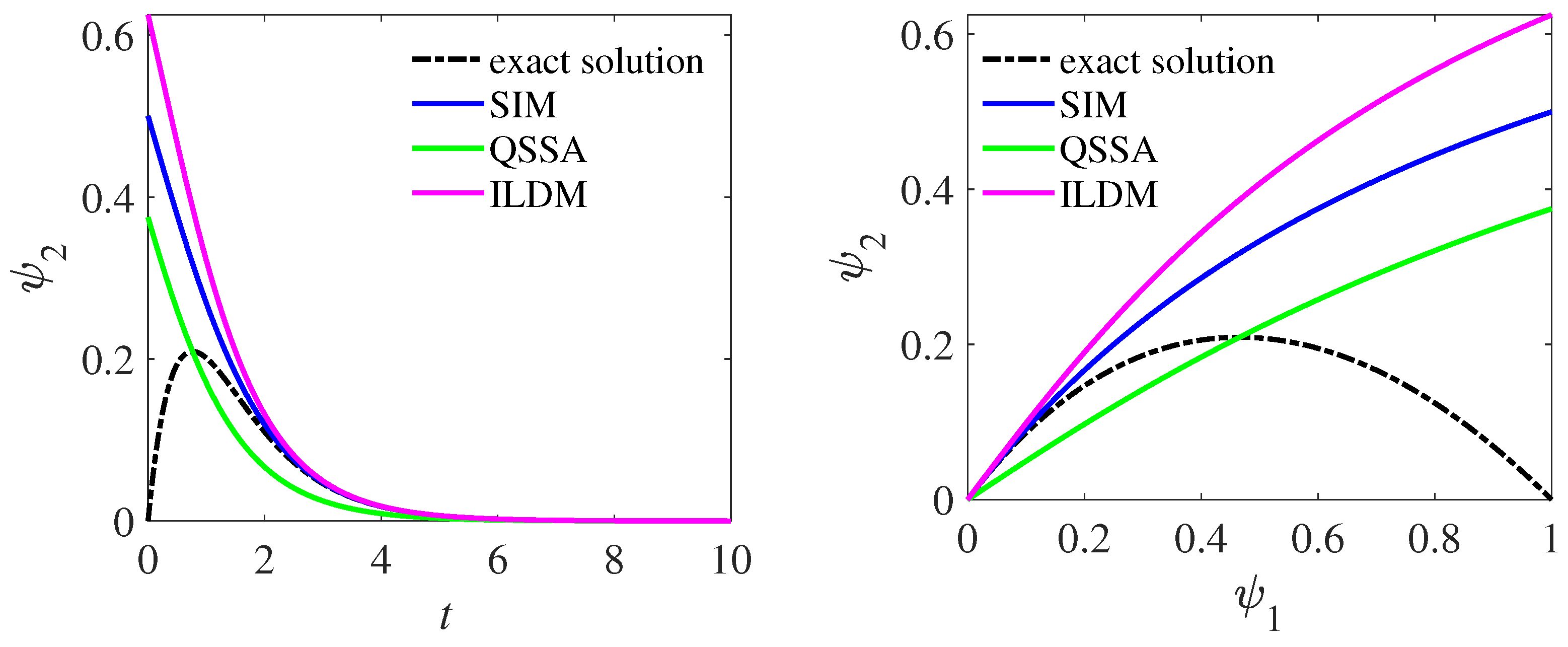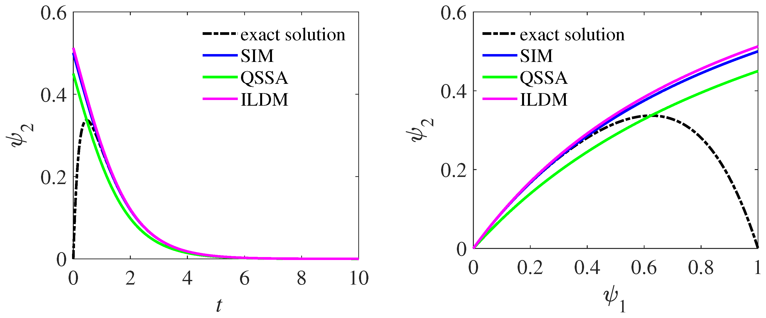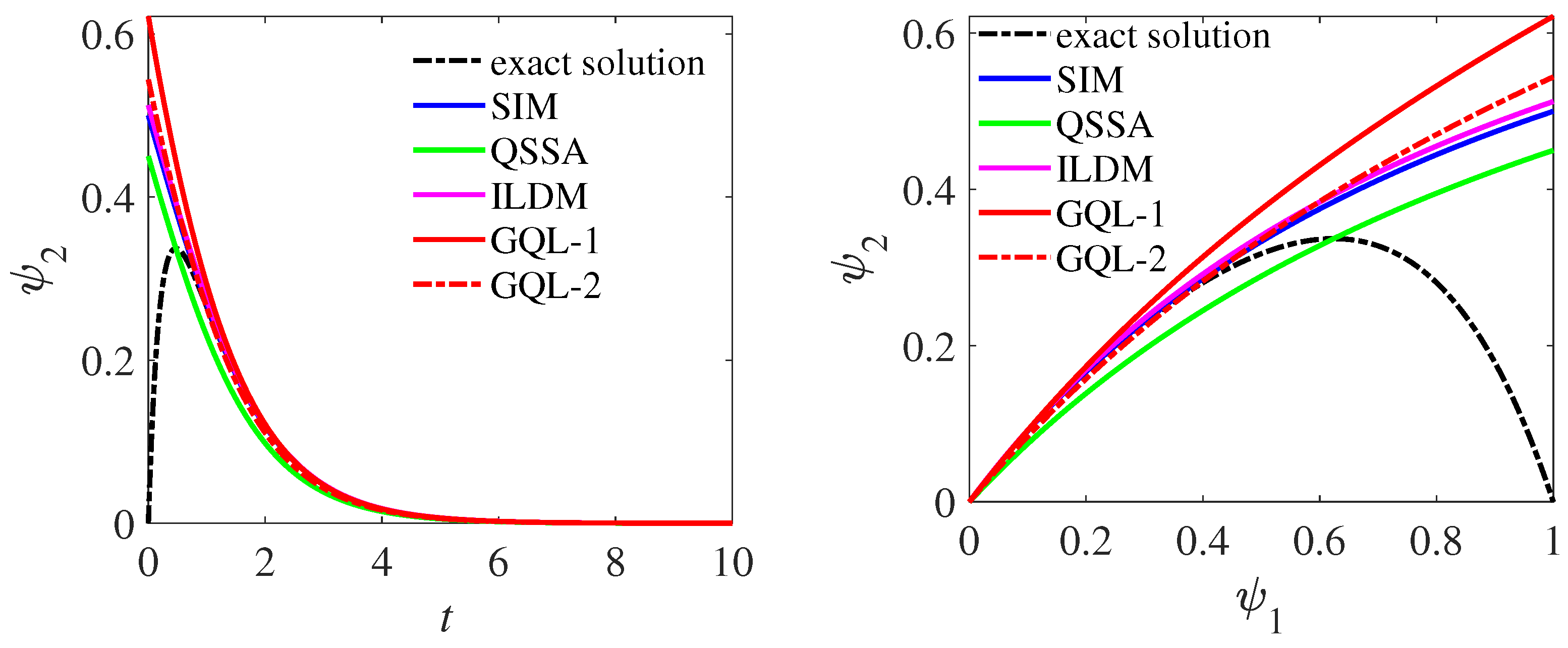Figure 1, Figure 2 and Figure 3 show the time development of ${\psi }_2$ (left) and the state space (right) by using the QSSA and ILDM method, compared with the exact slow invariant manifold (SIM) and the detailed solution. We notice that, as we already explained earlier, the slow manifold by small $\gamma$ (here $\gamma =2.0$ in Figure 1) shows inaccurate approximation by using the QSSA and less accurate approximation by using the ILDM. However, as $\gamma$ increases to a large value (here $\gamma =10.0$ in Figure 3), all manifolds almost overlap with each other, and even the QSSA gives a very good result. This indicates that, as discussed, for a large time scale separation, most reduction methods work very well, while for a small time scale separation, the conventional methods, such as QSSA here, fail to predict the slow manifold accurately.

Another interesting point must be emphasized here. Since the initial conditions are usually not located on the slow manifold, the errors of using a slow manifold at the initial time could be large. Dynamically speaking, the initial conditions will be relaxed onto the slow manifold, and then move along the tangential subspace of the slow manifold. For a large time scale separation (e.g., Figure 3 with $\gamma =10.0$), the time scale for fast relaxation is very fast compared with the time scale for a slow process; therefore, the whole process is dominantly controlled by a slow process, and the time development of ${\psi }_2$ can be predicted solely by the slow process (slow manifold) sufficiently. However, for a small time scale separation (e.g., Figure 1 with $\gamma =2.0$), the time scales for fast relaxation and a slow process are in the same order of magnitude. Thus, both fast and slow processes are important for the description of ${\psi }_2$, and the dynamic of ${\psi }_2$ described solely by a slow process (slow manifold) is not sufficient. Generally, there are two approaches to deal with the initial conditions:

• The dimension of the slow manifold can be increased so that the initial conditions are closer to the slow manifold. Consequently, the errors at the initial stage will be reduced. However, for the proposed Davis–Skodje model, the increase in dimension of a slow manifold is not possible.
• The fast process can also be identified by the GQL approach. According to the GQL concept, during the fast process, the initial conditions relax onto the manifold in the direction where the value of slow variables does not change. Mathematically, one can formulate the algebraic equation at the initial stage as ${\tilde{Z}}_s\overrightarrow{\psi }={\tilde{Z}}_s{\overrightarrow{\psi }}_0$, where ${\psi }_0$ is the initial condition. However, the identification of the fast process by other methods, such as the QSSA and ILDM, is not considered in their corresponding work.

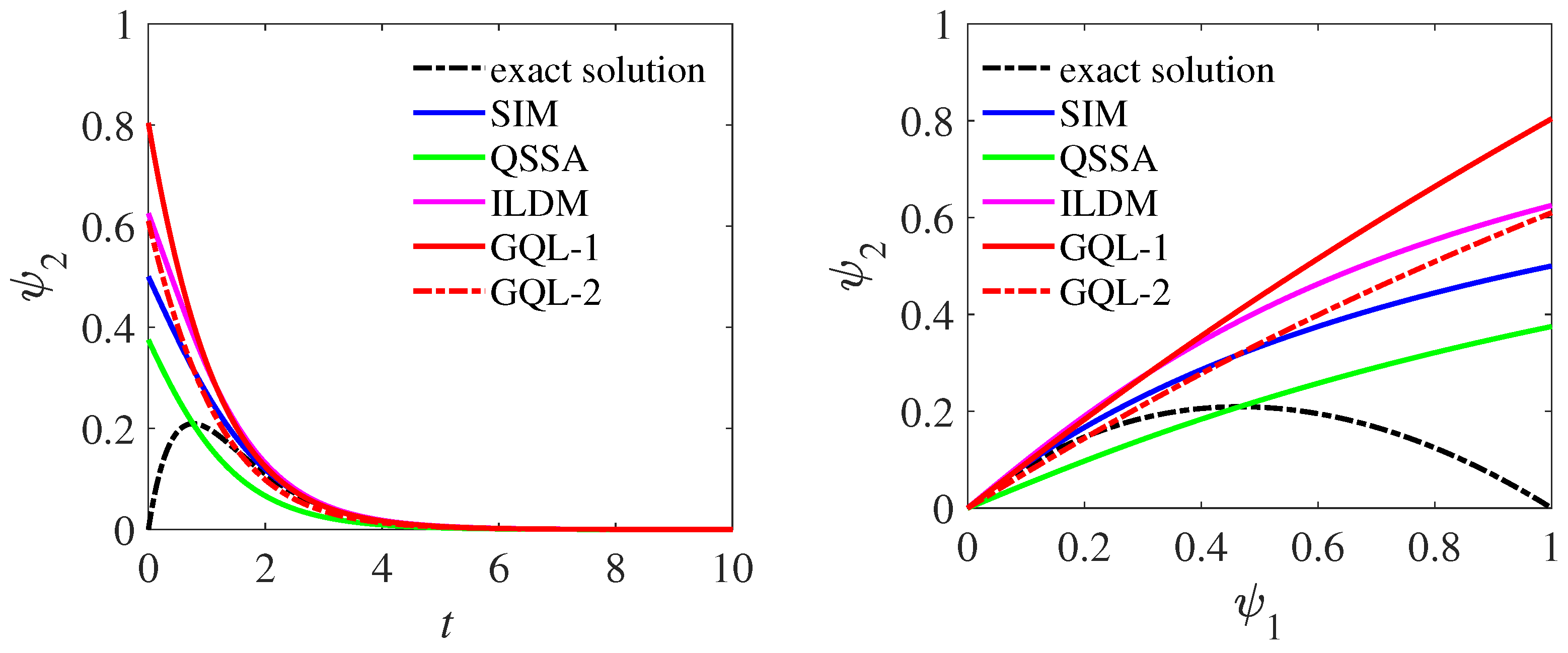
3.2. Application of the GQL

Now, the procedure proposed in [12] is implemented, and the GQL is computed. The latter is based on the local Jacobian, which can be used to approximate the global linearization matrix ${\mathbf{T}}_{\mathrm{GQL}}$ due to the mean value theorem. The local Jacobian of the source term $\overrightarrow{F}$ can be determined analytically:

$$\mathbf{J}=\left(\begin{array}{cc}{J}_{11}& J_{12}\\ J_{21}& J_{22}\end{array}\right)=\left(\begin{array}{cc}-1& 0\\ \frac{\gamma -1+(\gamma +1){\psi }_1}{{(1+{\psi }_1)}^3}& -\gamma \end{array}\right),$$

(15)

leading to the left eigenvectors:

$$\left(\begin{array}{c}{\tilde{Z}}_s\\ {\tilde{Z}}_f\end{array}\right)=\left(\begin{array}{cc}1& 0\\ -\frac{\gamma -1+(\gamma +1){\psi }_1}{(\gamma -1){(1+{\psi }_1)}^3}& 1\end{array}\right).$$

(16)

If the fast invariant subspace is given as ${\tilde{Z}}_f={(Z_{f1},Z_{f2})}^{\mathrm{T}}$, then the GQL slow manifold is

$${\mathcal{M}}_{GQL}=\{\overrightarrow{\psi }:{\tilde{Z}}_f·\overrightarrow{F}\left(\overrightarrow{\psi }\right)=Z_{f1}·{\mathrm{F}}_1\left(\overrightarrow{\psi }\right)+Z_{f2}·{\mathrm{F}}_2\left(\overrightarrow{\psi }\right)=0\}.$$

(17)

Following the GQL algorithm, the basis for the GQL decomposition can be computed at representative states. Two different GQLs are selected for further consideration and discussion. Both ${\mathbf{T}}_{\mathrm{GQL}}$ are given as

$${\mathbf{T}}_{\mathrm{GQL}\text{-}1}=\left(\begin{array}{cc}-1.0& 0.0\\ 4.1172& -5.8\end{array}\right),{\mathbf{T}}_{\mathrm{GQL}\text{-}2}=\left(\begin{array}{cc}-1.0& 0.0\\ 1.3252& -3.82\end{array}\right).$$

(18)

For the generation of the GQL reduced chemistry, the target quantity is selected as the ${\psi }_2$ value at $t=2$. Both GQL candidates are so selected that GQL-1 has a larger user-defined error (5%) and GQL-2 a smaller user-defined error (2%). Note that, here, this selection of target quantity is arbitrary, and other target quantities of interest can be chosen. Additionally, the user-defined errors here are also arbitrarily selected, and the main purpose is only to show how the quality of the GQL matrix is affected by the user-defined error. Figure 4 and Figure 5 show again the time evolution and phase plane for $\gamma =2.0$ and $\gamma =5.0$, together with the above-mentioned two GQL candidates. We observe clearly that both GQL reduced chemistries are valid candidates, and for $\gamma =5.0$, both GQL candidates give good results. GQL-2 (with smaller user-defined error) is almost identical to the SIM and ILDM results. GQL-1 (with larger user-defined error) gives also an accurate result near the equilibrium point. For both GQL candidates, they are much accurate than the QSSA trajectory.

3.3. Some Conclusions and Comments

In this section, the simple Davis–Skodje model has been demonstrated to discuss different reduction methods, namely, SIM, QSSA, ILDM, and GQL. The variation effect of time scale separation, namely, the parameter $\gamma$, has been investigated. It was shown that the larger the time scale separation is, the better the performance of the reduction methods is. For a small time scale separation, where the QSSA fails to give an accurate slow manifold, the GQL can still give good prediction and has a similar accuracy as the ILDM method. Additionally, these conclusions are also valid for the more complicated system proposed in the following two sections.

4. Results and Discussion: Hydrogen–Air Homogeneous Reaction System

In this section, the hydrogen–oxygen isochoric homogeneous reacting system is considered a simple but representative example. This system has a total of 11 dimension, including 2 thermodynamic parameters and 9 reactive species. It has been intensively investigated in our previous works [12,16], showing the advantage of the GQL over the QSSA for leading order approximation. There, and also in other previous works, one looks for an optimal GQL reduced model. In this part, the GQL reduced chemistry used in [16] is applied to test a wider range of applications and different combustion system configurations. The target quantity to define the error of the GQL reduced model is based on the comparison of ignition delay time, an important quantity describing the reactivity of the combustion system.

4.1. Isobaric Homogeneous Reacting System

In this part, results are demonstrated by using an optimized 4D GQL reduced model. The 4D GQL reduced model is optimized such that the relative errors of the reduced solutions for the user-defined range of interest (initial temperature 800 K $\le T_0\le$ 2000 K, pressure $p_0=1$ bar, fuel/air equivalent ratio $\Phi =1.0$) are below 2%. This 4D GQL reduced model has been validated in our previous work [16] for an isobaric homogeneous reacting system. Now, it is shown that it also works for a much wider range of system parameters.

In Figure 6, therefore, several representative predictions of ignition delay times (IDTs) are shown by using a detailed chemistry (symbols) and GQL reduced model (solid lines) and the corresponding relative errors of the reduced solutions as well. It is shown that even if the GQL reduced chemistry is optimized for a system with $p_0=1$ bar and a stoichiometric mixture only, it also works for higher pressures and other fuel/air equivalent ratios. However, the same isobaric homogeneous reacting system is considered. Remark that the relative errors grow, reaching a maximum of around 8% at high initial temperatures. However, it should be emphasized that such relative errors can be further reduced, if one considers these ranges in the optimization of GQL reduced chemistry.

4.2. Isochoric Homogeneous Reacting System

The GQL reduced model is now tested for the homogeneous reacting system under an isochoric condition. Such test can further support the observation made that the GQL is invariant with respect to the change of system parameters. This extends the observation made that the GQL is invariant with respect to the mechanism as it was demonstrated in [16].

Figure 7 shows the predicted IDTs over initial temperatures based on detailed chemistry (symbols) and 4D-GQL reduced chemistry (solid lines), and the corresponding relative errors of the reduced results. Furthermore, the reduced model is also applied for four other mechanisms, and the maximal deviation between different detailed mechanisms is also shown in Figure 7 (right) for references. It should be mentioned here that the maximum deviation at some ranges is well beyond 20%, which is therefore not shown in the figure. In order to show the performance of the GQL reduced model, in Figure 8, the prediction of IDTs based on the QSSA for O and OH as QSS species was implemented, which has been also validated in [12]. Several major observations can be drawn, namely,

• The 4D QSSA reduced model, which considers O and OH as QSS species, provides similar accuracy for different mechanisms. Such QSSA is reasonable for low temperatures, but gives high errors (around 15%) at high temperatures (similar order of magnitude as maximal deviation between different mechanisms).
• The GQL reduced model, which is optimized for an isobaric system, works also for an isochoric system. The relative errors of the reduced results are much smaller than the deviation between different mechanisms for the whole temperature range.
• Consistent with our earlier observation in [16] in which the isobaric system is considered, the GQL reduced model, which is optimized for one mechanism, is also valid for other mechanisms. We see that the errors are well below 5% in Figure 7. This shows the intrinsic property of the chemical reactions that the invariant subspace is not dependent on the mechanism.

Figure Figure 9 gives more results by applying the same 4D GQL reduced model for different mechanisms under different pressures and fuel/air equivalent ratios for an isochoric system, which additionally confirm the observations mentioned above.

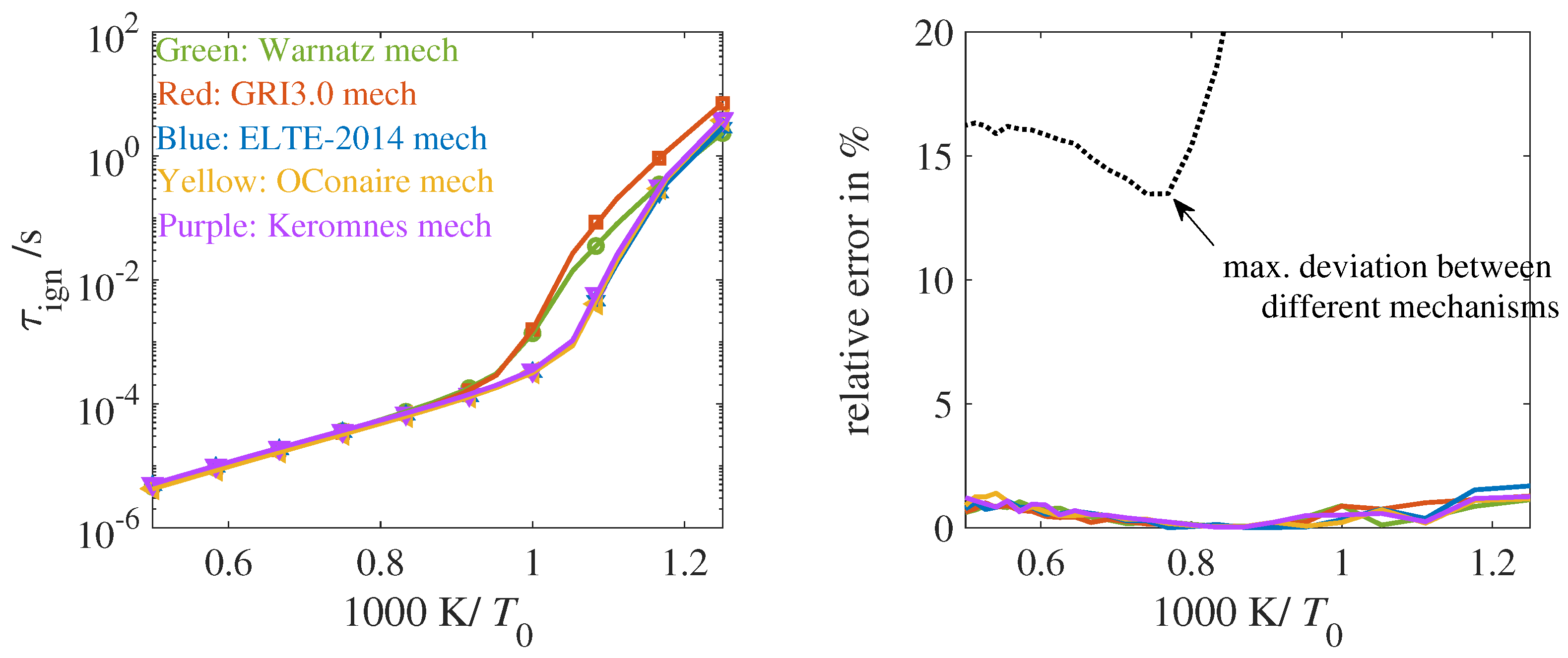
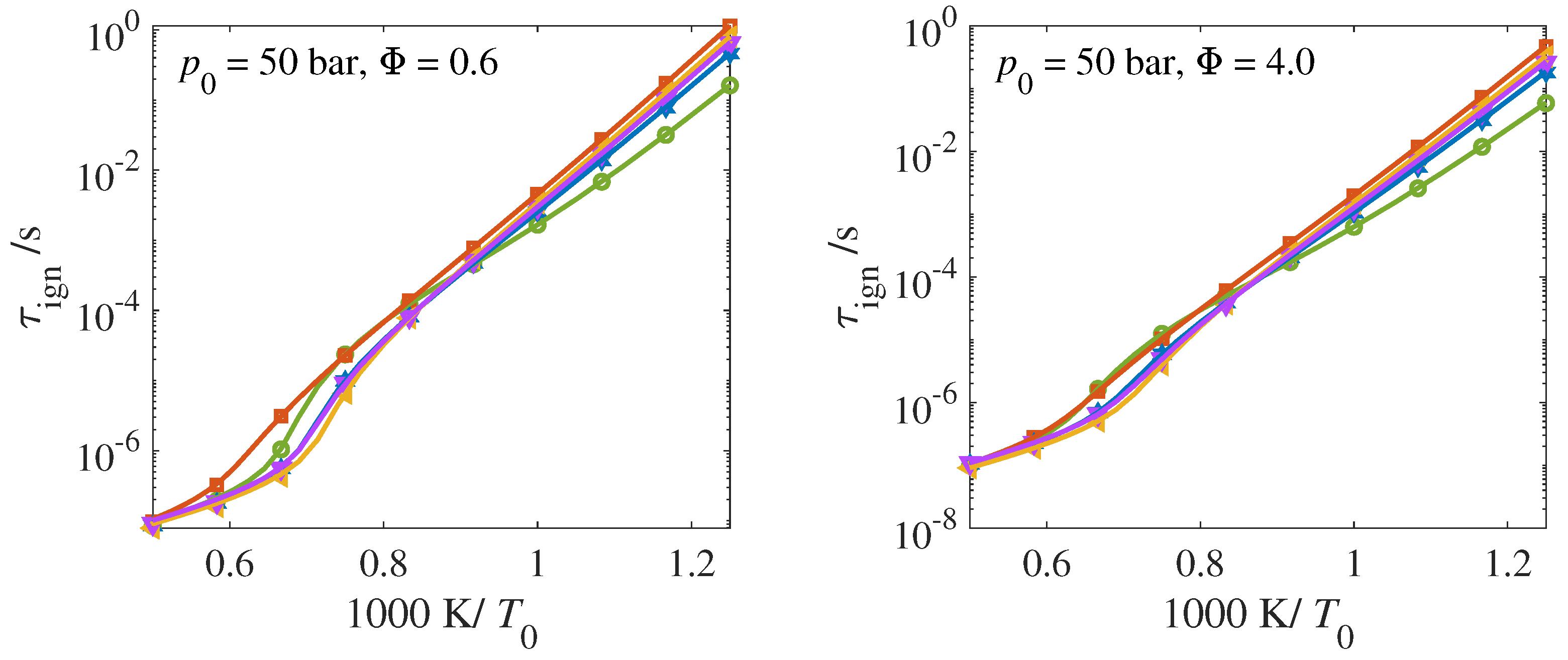
5. Results and Discussion: Ethanol–Air Homogeneous Reaction System

The hydrogen–air combustion system discussed in the last section provides some useful aspects for the performance of the GQL method. In this part, an ethanol–air combustion system is considered, which is considered low-carbon biofuel for the reduction of global CO${}_2$ emission [17,18,19]. The corresponding full chemical mechanism consists of 57 species [20]. The reduction for such relative large mechanism can be achieved in different ways, e.g.,

• The most general way is to directly use the QSSA or GQL to reduce the original full mechanism.
• Another possible way is to first generate the skeletal mechanism using, e.g., DRG-based methodologies [13,21,22] to reduce the number of species, and then use the QSSA to further reduce the dimension. The combination DRG-QSSA has been successfully applied in, e.g., [23].

In this section, the second way is explored; namely, the original full mechanism is first reduced to a skeletal mechanism with a smaller number of species using the DRG, and then the GQL is performed for this skeletal mechanism for further dimension reduction.

The DRG has been applied for the ethanol chemical mechanism, and the corresponding skeletal mechanism with 37 species (DRG-37D) is obtained in [24]. The skeletal mechanism has been tested for an autoignition process in terms of ignition delay times, premixed flat flames in terms of laminar burning velocity, and non-pre-mixed counterflow diffusion flames in terms of flame structure.

The GQL method is compared now with the standard QSSA method, as it was compared for hydrogen–air system above. The QSSA reduced results are also presented. From [25], the CSP approach confirms 10 QSS species: C${}_2$H${}_3$, CH${}_2$OH, CH${}_3$CHOH, CH, C${}_2$H, C${}_2$H${}_5$, HCO, CH${}_3$O, CH${}_3$CH${}_2$O, CH${}_3$CO. This results in a 23-dimensional DRG-QSSA reduced model, which is denoted as DRG-QSSA-23D in the following.

Furthermore, following the procedure in [12], a 14-dimensional GQL reduced chemistry has been obtained from the skeletal mechanism, and this is referred to as DRG-GQL-14D. This GQL reduced model has been so selected that tests for the whole studied temperature under $p=1$ bar and a stoichiometric mixture condition show all the relative errors of the predicted ignition delay time ${\tau }_{\mathrm{ign}}$ under 5% (note that other GQL reduced models can be obtained once other test conditions and relative errors are selected).

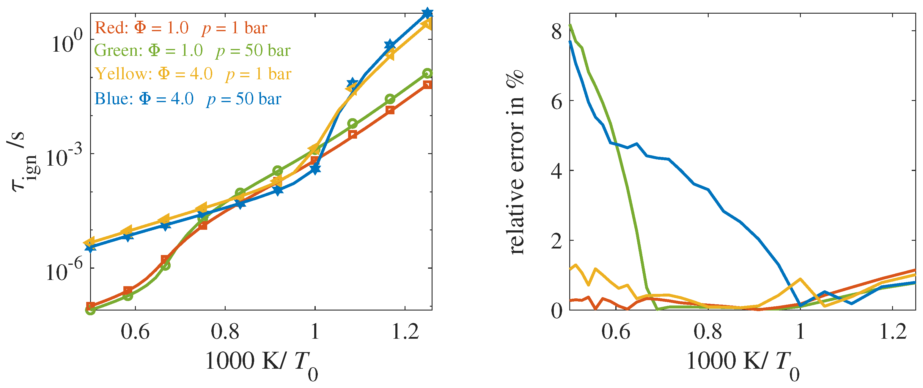
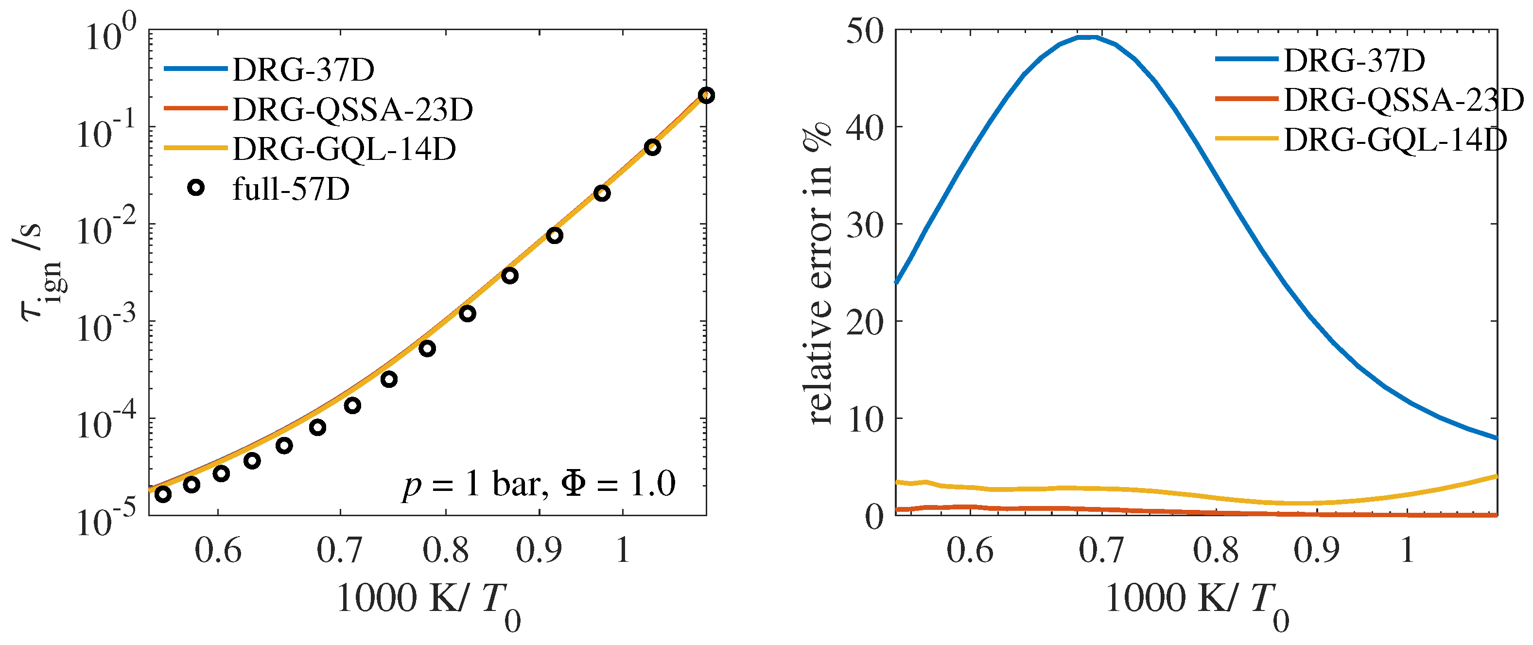
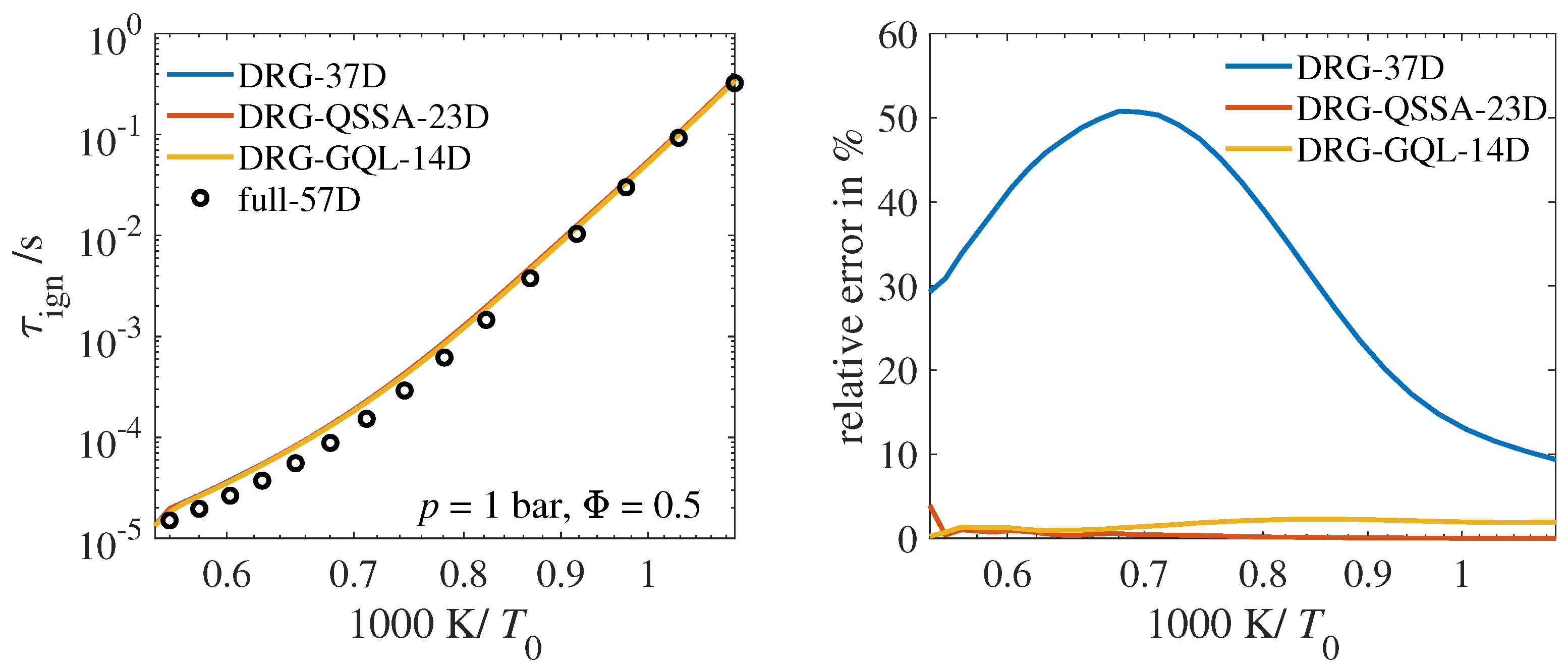
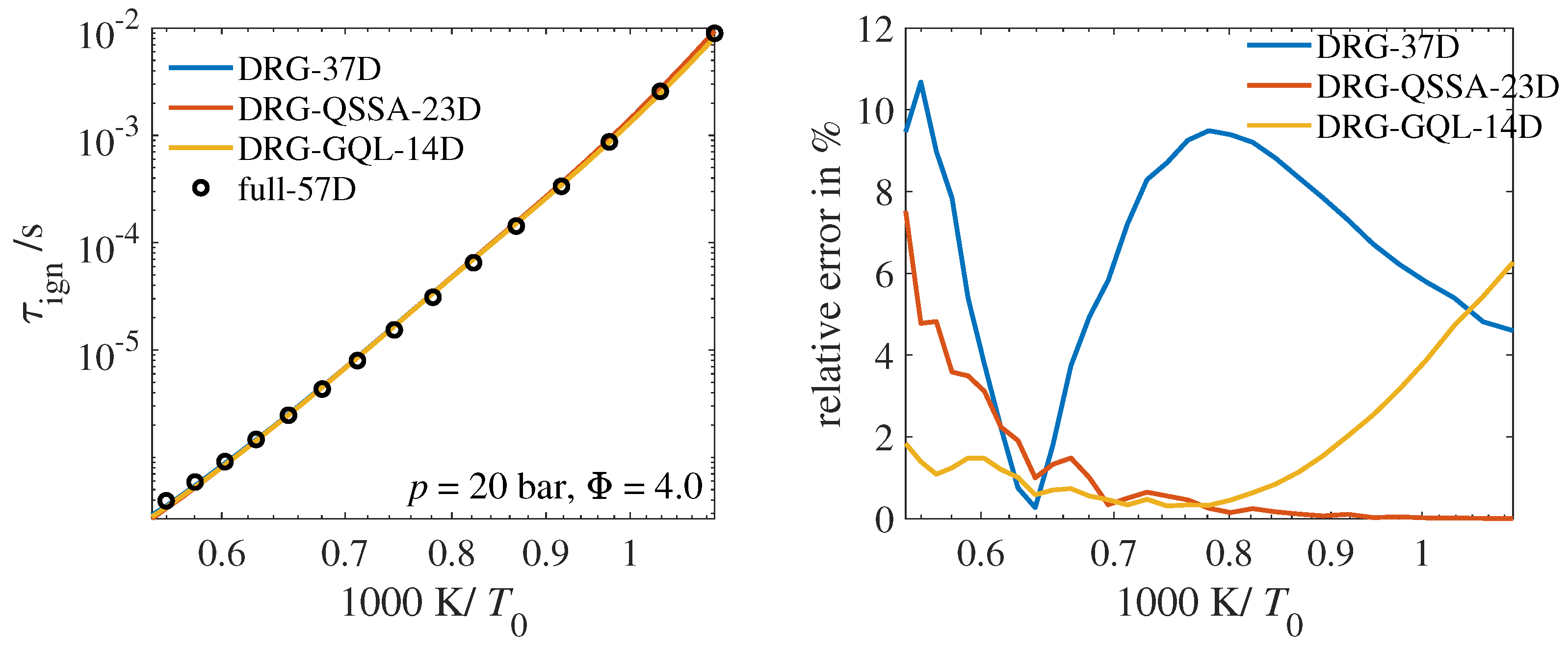
Figure 10, Figure 11 and Figure 12 show a comparison of the IDTs using 57-dimensional (57D) full chemistry and different reduced models. The relative errors are also presented to provide a direct comparison. Note here that the relative errors for DRG-37D are determined by referring to a full mechanism, and the relative errors for DRG-QSSA-23D and DRG-GQL-14D referring to a DRG-37D skeletal mechanism. Notice that the DRG-37D skeletal mechanism causes large errors, while the further reduction based on QSSA and GQL methods causes only additional 8% relative errors in these examples, much smaller than the errors induced by the DRG method implementation. It should be especially mentioned here that DRG-QSSA-23D has lower relative errors compared with DRG-GQL-14D, only because DRG-QSSA-23D has higher dimension. If the 23-dimensional (23D) GQL reduced chemistry is generated, the corresponding relative errors decrease dramatically. However, at some conditions, such as here for $p_0=$ 20 bar and $\Phi =4.0$, DRG-GQL-14D can also result in smaller relative errors compared with a DRG-QSSA-23D reduced model.

6. Conclusions

In this study, the global quasi-linearization (GQL) approach has been presented with a simple Davis–Skodje model and two practical/realistic homogeneous reaction systems: hydrogen–air and ethanol–air systems. The benchmark model has been used to illustrate the accuracy and the performance of the suggested approach to treat the systems when the assumption about an existing decommission is not asymptotically valid. It has been demonstrated how the GQL can be used to obtain the decomposition and the approximation for the slow invariant manifold automatically.

The ignition problem has been considered to treat practical combustion systems. The ignition delay times have been considered the representative quantities to quantify the performance of the GQL reduced models and compute relative errors for comparison. The GQL reduced model has been compared with the standard QSSA. For all three different (in terms of complexity and dimension) systems, the GQL better approximates a slow manifold and shows either higher accuracy than the QSSA or lower dimension than the QSSA, but with similar accuracy. Additionally, it was demonstrated how the DRG method, a representative method to generate the skeletal mechanism, can be applied in combination with the GQL. It has been shown that the DRG skeletal mechanism can lead to large relative errors. Though the GQL approach brings small additional errors, it considerably reduces the dimension. The suggested combination for the ethanol–air system in the autoignition problem reduces the full mechanism with 57 species to 37 species with the DRG, which is further reduced to 14 dimensions with the GQL.