1. Introduction
Subsea pipelines and cables in ice-prone regions are crucial components of offshore infrastructure for industries such as oil and gas production, electric power transmission, and telecommunications. However, in arctic and subarctic regions, these vital structures may face potential threats from icebergs, especially when pipelines are not buried and may come into direct contact with iceberg keels. Understanding the types and magnitudes of the interactions between icebergs and subsea cables is essential for assessing risks and developing effective mitigation strategies.
The study of cable damage by icebergs relies mainly on physical experiments [
1,
2], which provide the most accurate and reliable estimates of the interaction forces. Such tests are expensive, time-consuming, and challenging to conduct under controlled conditions that mimic the ice-structure interaction in the natural environment. Furthermore, these experiments are limited in the scales and shapes of the investigated samples.
Numerical modeling techniques have emerged as valuable tools for investigating various engineering problems. Techniques like finite element analysis (FEA) and cohesive zone (CZ) method offer established tools for numerical investigation of various engineering problems. This approach may allow researchers to simulate iceberg–cable interactions, explore various scenarios, and assess the resulting forces and damage.
Ice fracture presents a complex challenge for numerical modeling due to various fracture modes, such as crushing and spalling, which are inherently difficult to capture within a single modeling approach. Additionally, the random nature of fracture introduces significant uncertainties, making it impossible to predict the precise trajectory of every crack. Consequently, the primary objective of this work is to investigate the influence of geometric factors on the fracture process rather than predict the exact loads. By focusing on the effects of geometry, numerical models contribute to a deeper understanding of ice loads on subsea pipelines.
Cohesive zone models use a variety of traction-separation laws [
3], the simplest being a three-parameter bilinear cohesive law. The three parameters are (1) initial elasticity, (2) cohesive strength, and (3) fracture energy, which is the integral under the traction-separation curve. The fracture energy determines the maximal separation of the CZ that should be similar to the size of the fracture process zone. Cohesive strength is also known as failure stress or nominal stress and determines the maximum traction that CZ may transmit. Usually, there are separate values for normal and tangential cohesive strengths. Initial CZ elasticity has to be set significantly higher than the elastic modulus of the bulk material, otherwise the presence of CZs will decrease the average elastic modulus of the bulk material. While the shapes of traction-separation curves may vary significantly, the above-mentioned parameters are common for most formulations.
1.1. Related Work
Recent studies apply the CZ approach to model ice fracture. The works by Lu et al. [
4] and Wang et al. [
5] investigate the interaction between sloping marine structures and uniform ice sheets. In both works, ice is represented by triangular prism finite elements. There is one vertical layer of such elements, and all triangles are equilateral. Cohesive zones are inserted between the prism elements, allowing for crack propagation at 60° angles. The work by Lu et al. [
4] mitigates such anisotropy by randomizing the fracture energy of cohesive zones. While the simulation is three-dimensional, crack propagation is limited to two dimensions—The plane of the ice sheet. Such model limitation is reasonable, because it focuses on flexural ice failure.
Work by Kuutti et al. [
6] investigates ice sheet crushing from a different perspective. Here, the ice block is represented by an unstructured triangular mesh, with one vertical and one horizontal dimension. Cohesive zones are inserted between all elements, so the cracks can propagate parallel to the plane of the ice sheet. Since the mesh is unstructured, the fracture directions are not limited to specific angles. The work investigates how the simulation results are affected by the mesh size and the type of CZ formulation. The results are compared with laboratory studies.
The work by Gribanov et al. [
7] models the fracture of polycrystalline cylindrical samples under uniaxial loading. The ice is represented by three-dimensional geometry that is partitioned into separate polygonal grains. The grains are meshed by tetrahedral elements, and cohesive zones are inserted at grain boundaries. Due to the randomized nature of the grains, crack propagation is not limited to specific angles. One disadvantage of such an approach is its computational complexity due to the use of 3D meshes.
In the above-mentioned studies, the geometries, their scales, and the selected model parameters vary. Simulation parameters and characteristic sizes of the geometries are summarized in
Table 1. Elastic modulus and material density can be measured directly in experiments, but results may vary depending on the type of ice. Fracture energy could also be measured experimentally, but in the simulation, this quantity refers to individual cohesive elements rather than bulk material, so it does not directly correspond to measured values. Fracture energy should be higher than the experimentally measured energy of decohesion of two surfaces because a single cohesive element may represent a volume of material rather than a single surface. Finally, different studies use different values for the failure stress parameters, and such discrepancies are due to the differences in geometries, types of experimentally obtained data, and calibration approaches.
1.2. Experimental Data for Calibration
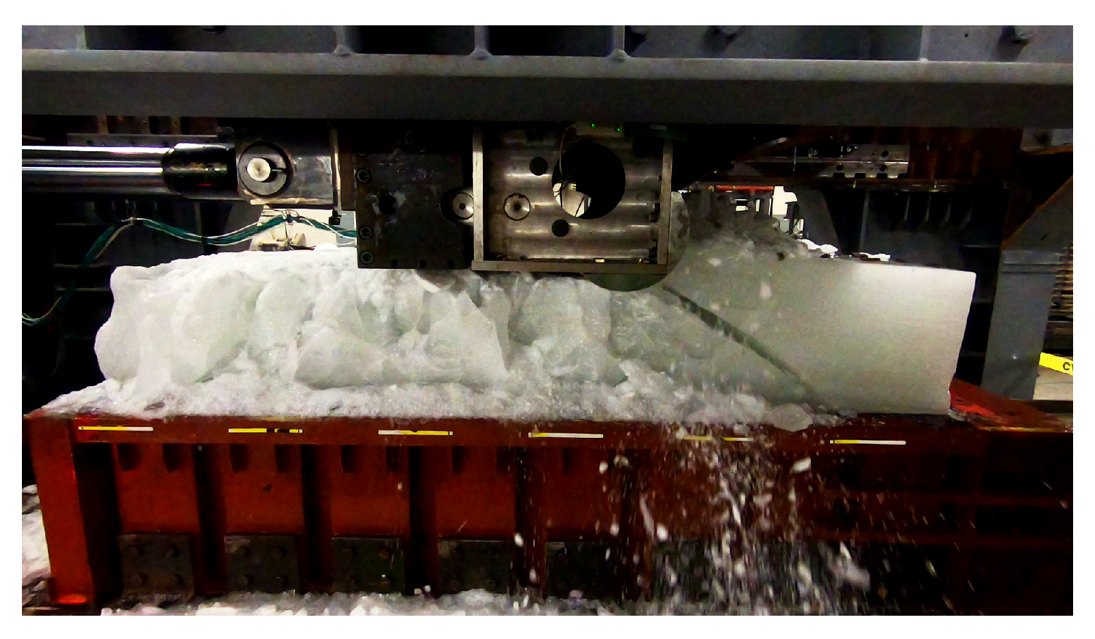
In a recent series of experiments, medium-scale indentation tests were conducted with rigid indenter and laboratory-grown samples of freshwater ice [
8]. The diameter of the indenter is 32.4 cm, which is intended to mimic a pipeline. The ice sample measures
cm (W × H × L), with the bottom half partially embedded in a confinement frame. Indentation rate is 20 cm/s, which is the typical speed of ice drift for the east coast of Canada. The indenter is driven by a set of accumulators, servo valves and hydraulic cylinders. The applied load is controlled to maintain the constant indentation rate.
Figure 1 shows the test apparatus with the ice sample at the conclusion of the experiment, and the characteristic end spall is visible on the right side of the block.
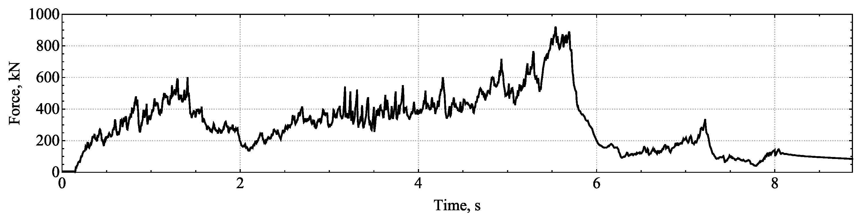
The testing apparatus is equipped with load cells, as well as tactile pressure sensors on the surface of the indenter. A typical reaction force plot is shown in
Figure 2, with the force magnitude exceeding 0.9 MN in this particular case. Several tests, including the one in
Figure 2, show gradually increasing force up until a large spall occurs at the end of the test. The vertical indentation depth is controlled by the height of the ice block sample. Out of nine conducted tests, six had an indentation depth of 2
(5.08 cm), two had a depth of 4
(10.16 cm), and one had a depth of 6
(15.24 cm). The values were selected by considering the capabilities of the testing apparatus, i.e., its power output. Experiments showed that the indentation depth in the studied range had no significant effect on the measured reaction forces [
8].
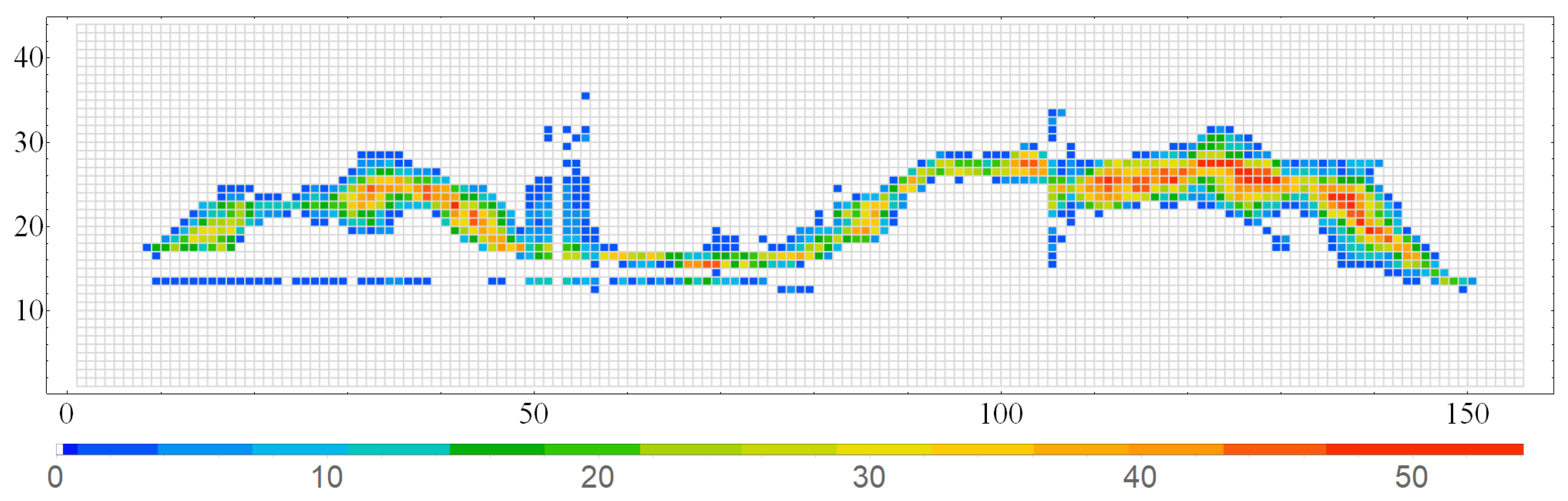
While most of the indenter’s surface is constantly in contact with the ice, the pressure on the surface varies. At the ice-indenter interface, the force is transmitted via several small regions, known as high-pressure zones [
9,
10]. A flexible pressure sensor was installed on the surface of the indenter. It consists of
elements (sensels) and covers > 95% of the ice-pipe interface.
As the indenter moves and comes in contact with intact ice, readings show rapid changes in pressure distribution on its surface. At any given time, typically a narrow region transmits the forces (
Figure 3). During the test, the angle of force application oscillates between nearly horizontal and nearly vertical. For model calibration, we rely on the data presented in
Figure 2 and
Figure 3, which are representative of the RHITA tests. Details about the remaining experimental tests are available in the publication [
8].
2. Formulation and Parameters
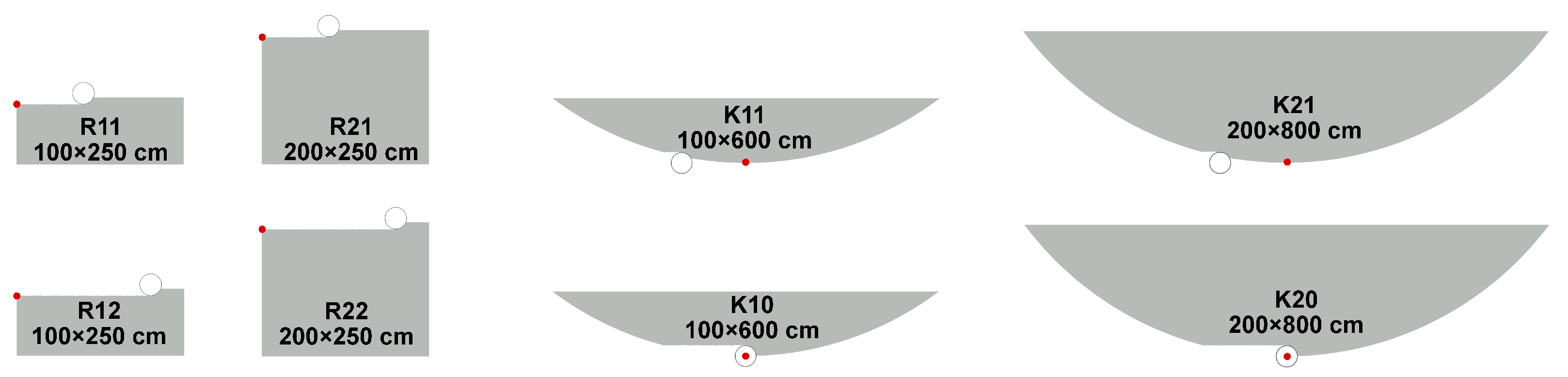
In this work, numerical simulations are carried out using the commercial FE package Abaqus with explicit time integration. A two-dimensional model is selected to maximize the resolution of the mesh and ensure adequate discretization of the surface curves. Two types of geometry are investigated—Rectangular blocks (R) and round keels (K).
Figure 4 shows the shapes with their corresponding codes, where the letter reflects the geometry of the sample, the first number is the height in meters, and the second number is the horizontal offset of the indenter from the axis origin. The goal is to estimate how different sample shapes and the indenter location affect the fracture force.
Sample shapes correspond to RHITA ice blocks that are halfway through the test. That is, an indenter crushed some of the intact ice, arriving to some midpoint on the surface of the block. Each investigated sample has surface of indenter contact with a diameter of 32.4 cm, to which the force is applied. The indentation depth for rectangular samples is 10.1 cm. For keel samples, the center of the indenter is vertically aligned with the bottom of the sample. The force is applied directly to the surface nodes with the magnitude linearly increasing at 10 MN/s. Fracture typically occurs at time between 0.05 and 0.20 s. Up until the point of fracture, the process is quasi-static, i.e., the sample remains immobile. The intent is to simulate a single fracture event somewhere in the middle of a RHITA experiment.
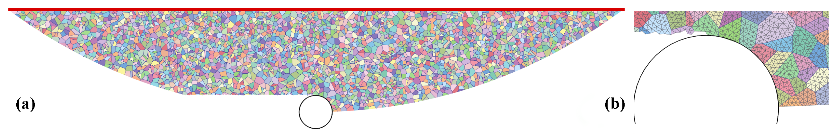
2.1. Mesh Generation
The investigated shapes are partitioned into a grain-like structure (
Figure 5). Due to computational limitations, the sizes of these grains are much larger than the typical sizes of natural ice grains. This tessellation and subsequent meshing are performed with open-source software Neper [
11]. Zero-thickness cohesive zones are inserted between the grains, and the resulting geometry is imported into Abaqus using a custom Python script. For each shape type, e.g., R11, R12, ten sample meshes are generated with the randomized arrangement of grains.
Table 2 shows the approximate node, element, and grain counts for each class. Element sizes and the number of grains were selected by considering the limitations of the computing hardware and the amount of compute time available. On one hand, higher resolution is desirable as it provides higher computation accuracy, more options for crack paths, and allows for finer fragmentation. On the other hand, finer mesh resolution results in longer compute time. In comparison with similar computational approaches [
4,
5,
6] that use structured grids with 60° angles, the non-structured grain geometry allows for more natural crack paths and, consequently, more accurate representation of the observed fracture phenomena.
Since the generated grain sizes are larger than that of natural grains, several consequences are expected. The main consequence is that the fragment size in the simulation is limited by the grain size, hence no crushing effects are reproduced in the simulation. As a result, the new surface area due to crushing in the model is lower than experimentally observed. The energy, which dissipates during crushing, must be accounted for in the simulation. The relevant model parameter is the fracture energy, and its value must be adjusted to account for the dissipation during crushing. Such an approach works well to capture large-scale processes, such as spalling.
2.2. Boundary Conditions
In the RHITA experiments [
8], the ice block is grown in a container that is one meter tall. Side walls are subsequently removed to expose the top half of the sample. The ice is bonded to the bottom of the container, but a gap remains between the ice and the remaining side walls, so the sides are not bonded. In the simulations, we impose the ‘encastre’ boundary condition on the bottom nodes to mimic the experimental setup. Similarly, keel shapes are constrained on their top side (
Figure 5a).
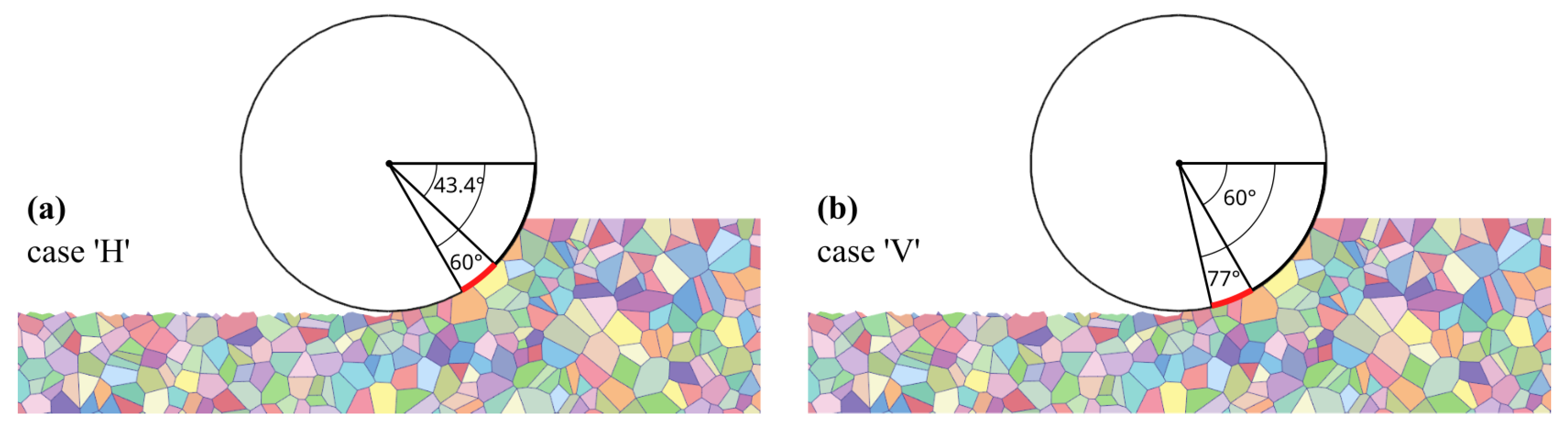
Two types of loading forces are investigated. In the first case, denoted as ‘H’ (more horizontal), the force is applied to the nodes between angles 43.4° and 60°. In the second case, ‘V’ (more vertical), the nodes are between 60° and 77° (
Figure 6). These angles were selected by inspecting Tekscan plots (
Figure 3) of several experiments. Typically, at least ten nodes receive the force application, which is distributed uniformly between the nodes. For keels, the angles of force application are the same, i.e., ‘H’ is the horizontal case, and ‘V’ is the vertical case with the same angles.
The experiments showed that the force is applied at angles from almost vertical to nearly horizontal. By selecting the fixed ‘V’ and ‘H’ cases, we intend to investigate how the application angle affects the maximal force that a sample can sustain.
2.3. Mathematical Framework and Parameter Selection
Abaqus is a closed-source tool, but some information about its inner workings is provided in its user’s manual. For example, the explicit time stepping uses the central difference integration rule, also known as leapfrog integration:
Here, denotes the nodal displacement vector, and its subscript denotes the time step number. Mass matrix is lumped for computational efficiency. Applied and internal forces are denoted as , and the time step is . The forces are computed according to the elastic response of the bulk elements, i.e., triangular elements that represent the material, and the response of cohesive elements.
For the scales and speeds considered in this analysis, ice may be reasonably approximated as a linearly elastic material. Cohesive zones limit the maximal applied load and, consequently, the maximal deformation of the bulk elements. Given that the deformation is small, the linear elastic model performs similarly to any other formulation of elastic behavior.
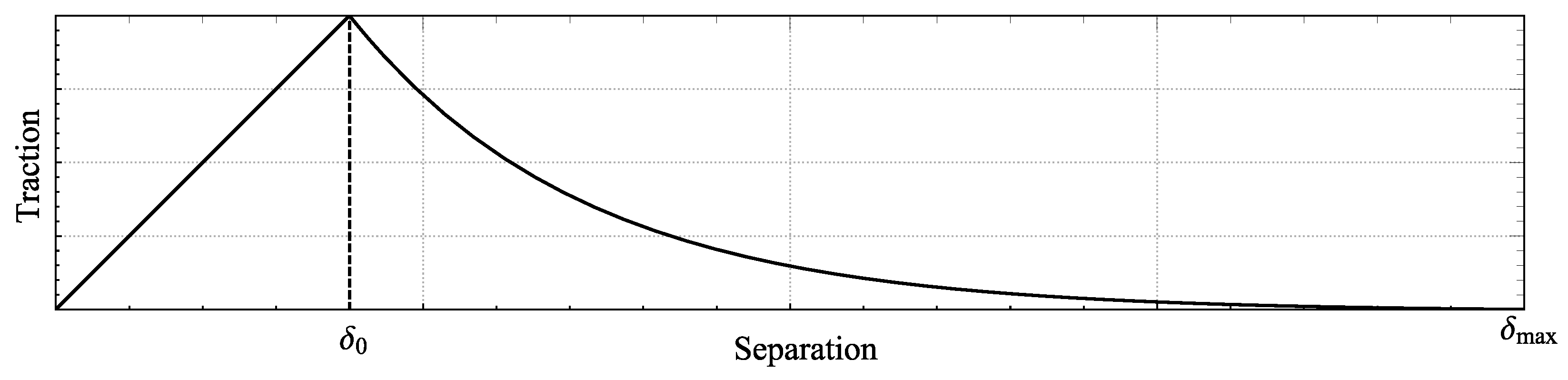
Abaqus provides a variety of formulations for cohesive zones. This work uses CZs with linear elastic traction-separation behavior, maximum nominal stress criterion for damage initiation, and exponential damage evolution. Linear traction-separation behavior is formulated as
where
is the linear traction function,
is the opening (separation) of the cohesive zone, and
is the initial CZ elasticity in the normal direction (for simplicity, this discussion only considers the normal direction). The influence of damage is given by the following expression:
where
is the resulting traction, and
D is the damage function, whose form depends on the damage model, damage initiation criterion, and CZ loading history. In the maximum nominal stress criterion, the damage function is zero until the traction reaches a given threshold—Failure stress. After passing the threshold, exponential damage evolution is given by the following equation:
where
is a dimensionless parameter that affects the shape of the traction-separation curve,
is the opening distance at which the CZ fails,
is the separation at which the maximum stress threshold is reached (the elastic limit of the CZ), and
is the maximal opening that a particular CZ ever reached (each cohesive element keeps track of this parameter separately).
The resulting traction-separation curve (
Figure 7) consists of the initial elastic range (separation below
), and the softening part (separation up to
). In Abaqus, the user does not directly specify the parameters
and
. Instead, they are calculated from the initial CZ elasticity
(the slope in the elastic portion of the curve), maximal stress, and the fracture energy
. The latter is the area under the traction-separation curve and represents the energy of surface decohesion. Parameters must be selected in such a way that allow the softening portion of the curve to be present. Also, the maximal opening of the cohesive zone
cannot be too large, as that would cause non-physical forces in the simulation.
Table 1 shows the range of cohesive zone parameters used in the previous studies. The values vary because the strength and density of natural ice also vary. Additionally, the scale of the studied geometry may affect the fracture energy
. Experiments showed that both freshwater and sea ice have a constant specific fracture energy
[
12]. Therefore, the parameter
should be adjusted depending on the area of cohesive zones per volume of the material. The selected model parameters are summarized in
Table 3.
Failure stress parameters (both tension and shear) directly affect the fracture force of a sample. That is, adjusting these parameters by a given amount would affect all simulations in a similar way. The values are selected to match the experimentally recorded fracture forces, but we only aim to set one significant figure for each parameter.
2.4. Post-Processing
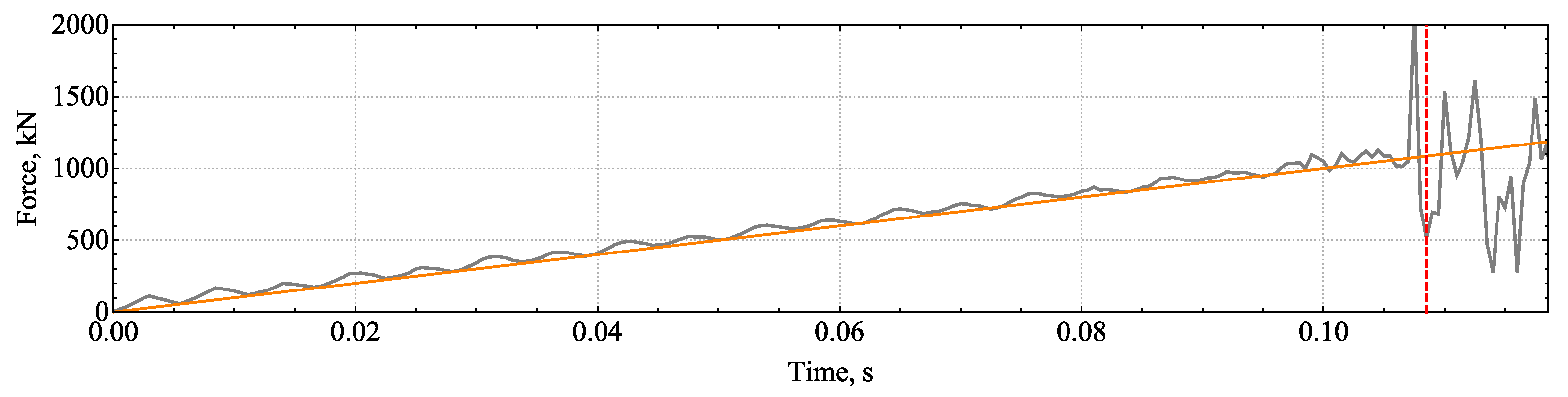
The applied pressure temporarily drops after each fracture event during the experiment. In the simulation, the force is applied directly to nodes and continues to be applied after the fracture event. Because of this, the results after the fracture event are not considered in the analysis. However, detection of the moment of fracture and the corresponding maximal force is necessary. After the computation job is finished in Abaqus, the results are exported to a custom binary format and analyzed with custom software. In particular, we export mesh displacements, per-element stress values, damage level of cohesive zones (‘SDEG’ parameter), and the active/failed state of cohesive zones (‘STATUS’ parameter).
The moment of sample failure is visually apparent, but we formalize the fracture detection algorithm to exclude subjective judgment. The approach is to compare the reaction force of the constrained surface of the block (
Figure 5) to the applied force at the indentation site. The fracture is detected when the reaction force is lower by 20% than the applied force. Such an event means that the indentation site is fragmented, and the fragments no longer transmit the indentation force to the block. To ensure that fragmentation is present, at least one cohesive zone is required to be broken. The complexity of the fracture detection algorithm arises from the noise and oscillations of the reaction force plot (
Figure 8).
3. Results
For each of the shape types (
Figure 4), ten samples with randomized grain arrangements are generated. Samples are subjected to two types of force application (
Figure 6), denoted as ‘H’ and ‘V’.
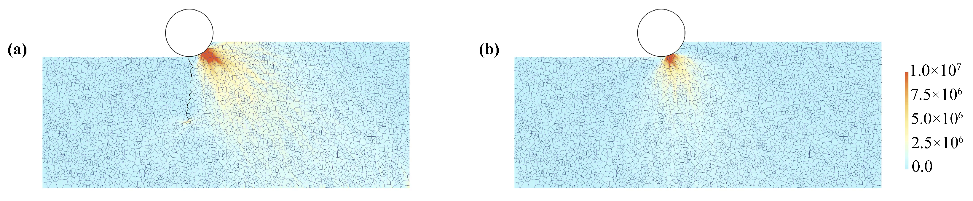
Figure 9 illustrates typical stress distributions just before fracture in the same sample but with different angles of force application. Results of the simulations are listed in
Table 4 for rectangular samples and in
Table 5 for keels. Detailed statistical analyses of the sample groups are presented in subsections below.
The results show substantial variability of fracture forces within the defined batches. For example, batch K21H has fracture forces that range from 905 kN to 1690 kN (
Table 5). Within the same batch, all simulation parameters remain constant except for the geometrical arrangement of grains. Natural and laboratory-grown ice has variability in its structure as well. Depending on the growth conditions and other factors, there may be imperfections, inclusions, and variations in grain structure, among other things. One can expect a certain degree of variability in the material itself.
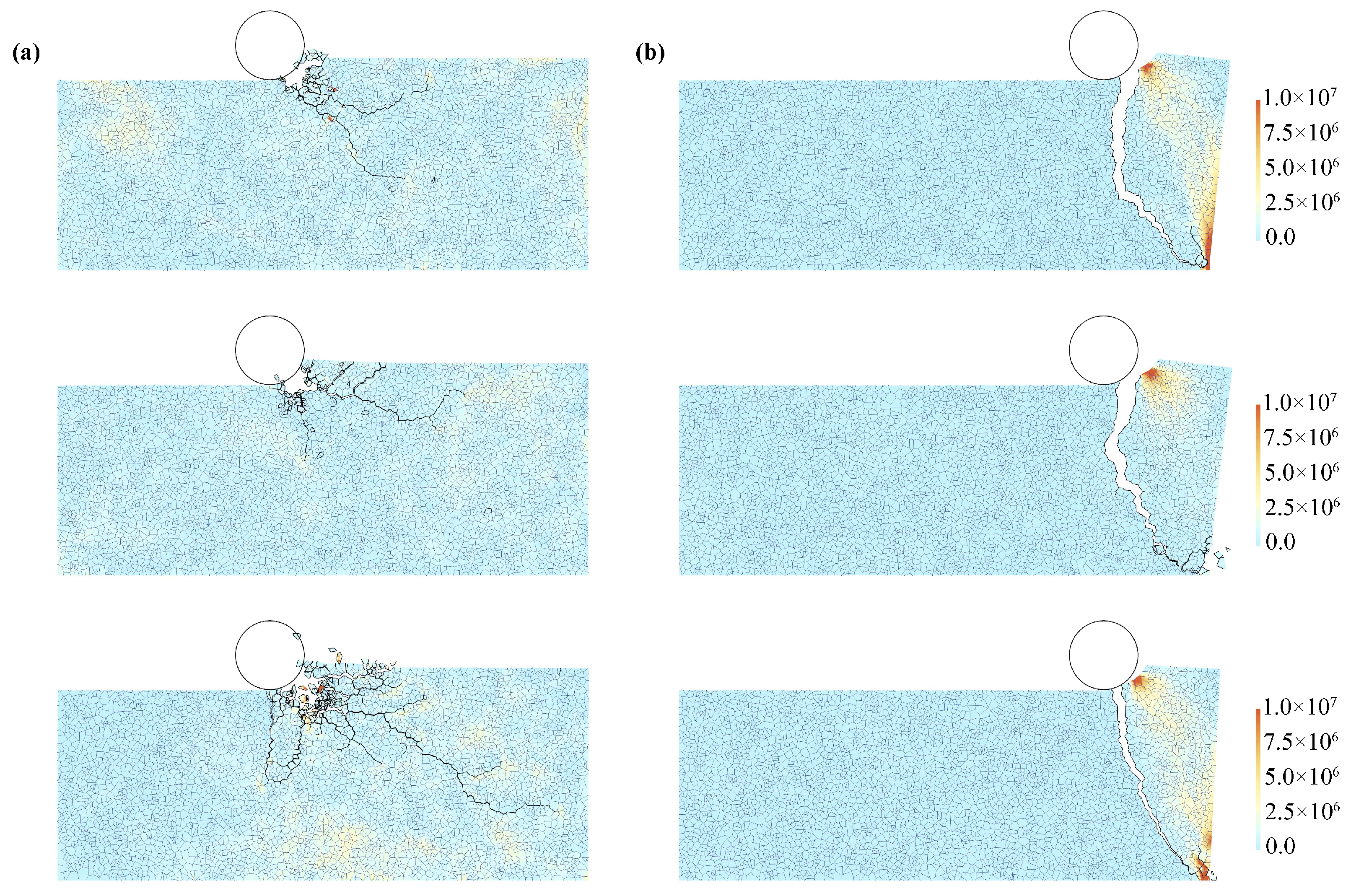
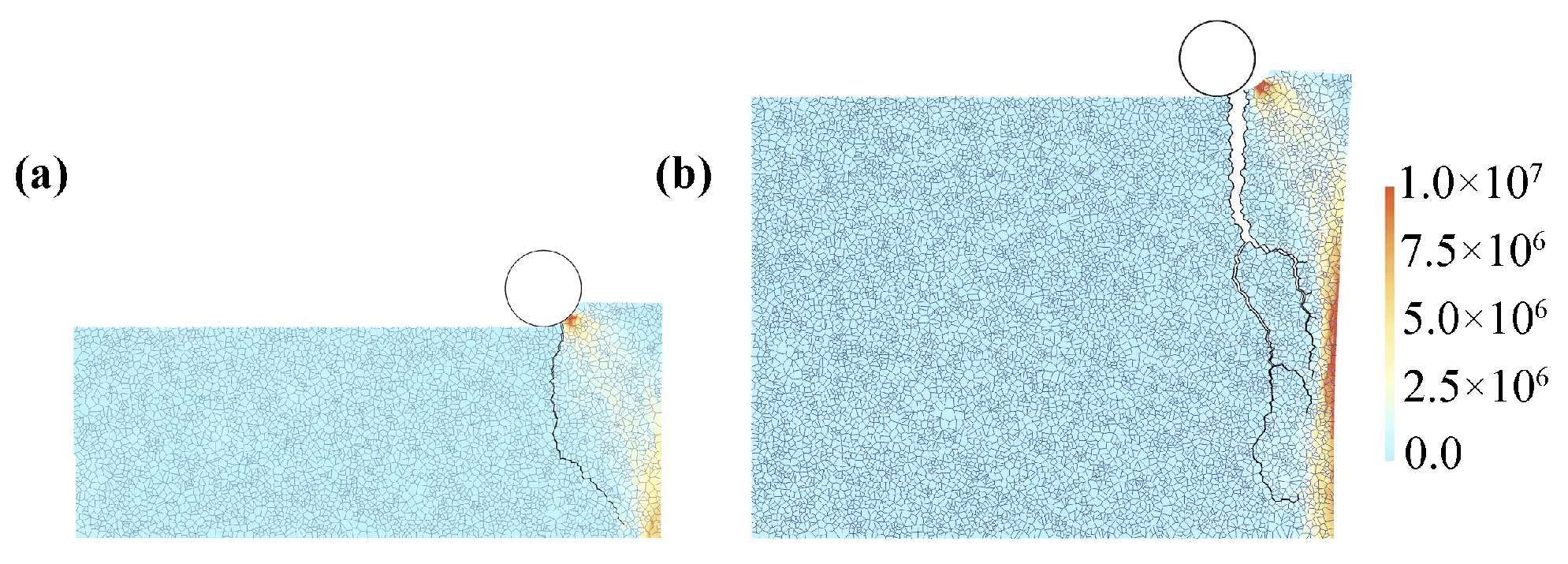
3.1. Rectangular Sample Groups
The mean fracture force for batch R11H is 1174.0 kN, whereas the fracture force for R12H is only 494.6 kN. Performing a
t-test on these two groups shows a statistically significant difference between the fracture forces (for this and subsequent tests, the
p-value threshold is set to 0.05). In group R11H, the indenter is positioned near the block’s horizontal center, acting against the bulk of the material. As a result, high fragmentation is observed (
Figure 10a) in this group.
On the other hand, group R12H has the indenter positioned at the right side of the block, making the fracture process different. A spall develops on that side (
Figure 10b) with a predictable shape and size. The predictable nature of such an event is reflected in the standard deviation values. For group R11H, the standard deviation is 235 kN, whereas group R12H has a standard deviation of only 82 kN.
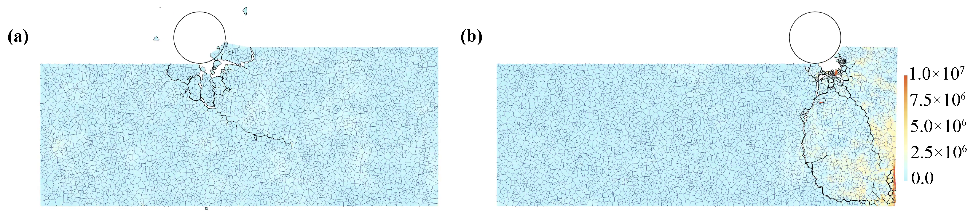
The effect of indenter proximity to the free edge does not always play a role. For example, the effect disappears when the force is applied more vertically (
Figure 11).
t-test does not show any statistically significant difference between the groups R11V and R12V. One can assume that the absence of the spalling event affects the fracture force and, consequently, the outcome of the
t-test.
During the experiments, frequent changes of the angle of force application are observed as the indenter moves. When the indenter reaches the right side of the block, it is likely that, at some point, the force will be applied horizontally, and a spall will happen. Such a spall was observed frequently during RHITA tests (
Figure 1).
3.2. Influence of Force Application Angle
Here, ‘H’ forces are compared against ‘V’ forces. Paired
t-tests are performed since the samples remain identical (same shape and grain arrangement). The results of these comparisons are summarized in
Table 6. For rectangular geometries R12 and R22, the proximity of the indenter to the free edge and the formation of a spall explains the low fracture force. The angle of force application controls whether a spall is created; thus, no significant difference is detected when the force is applied at a more vertical angle.
One of the keel-type geometries also shows the influence of the force application angle. The effect is only present for shape K10—The keel of the size
m, with the indenter located in the center (
Figure 12). Given that the taller keel groups do not exhibit any statistically significant influence of force angle, one can assume that the height of the keel (1 m) and the proximity of the fixed boundary (upper edge) play a role in this effect.
3.3. Influence of Block Height
In RHITA tests [
8], the maximal height of an ice sample is approximately 1 m, and the experiments provide accurate measurements of the fracture forces for such samples. However, the question remains about the relevancy of these data to the fracture of actual icebergs. Hence, it is beneficial to investigate the matter with numerical simulations.
t-test comparisons of one-meter and two-meter blocks are presented in
Table 7. Out of four group pairs, only one shows a statistically significant difference in the fracture force (
Figure 13). In groups R12H and R22H, the indenter is located closer to the end of the block, and a spall is likely to develop. While the difference in the mean fracture force is detectable, its relative value is less than 10%. Such a difference is not relevant to real-life scenarios. Simulations predict that the increase in the size of the testing apparatus would not affect the measurements of the ice fracture forces.
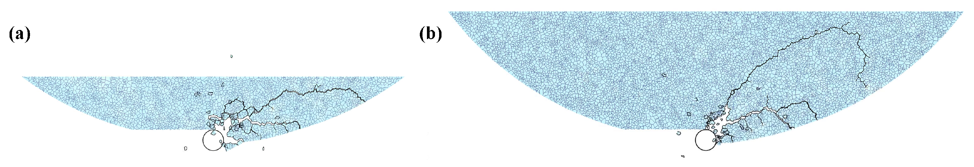
3.4. Comparisons of Keel Groups
While the experiments provide valuable data about rectangular blocks, interaction with a subsea cable would likely occur with keel-shaped ice. Iceberg keels come in various shapes, and there is no single solution to encompass them. Still, the simulation of a rounded shape may provide additional information compared to rectangular shapes.
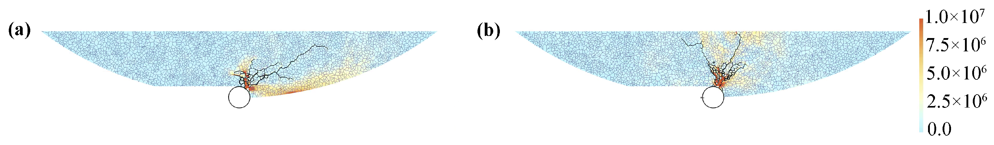
Here, we look at the influence of the keel height. Since the keel is round, horizontal dimensions also depend on the height of the keel.
Figure 14 shows that the fracture region extends up to the fixed boundary of the keel in both cases. However, the data show no statistically significant influence of the keel height on the fracture forces. Simulation results are summarized in
Table 8. Unlike the rectangular blocks, keels have no ’end spall’ event, so the fracture forces remain consistent and high.
4. Discussion
While the laboratory tests provide valuable and accurate data for medium-scale indentation [
8], there is a concern that readings may be different for larger-scale processes. By performing numerical simulations, we investigate how the changes in sample height, indenter position, and force application angles affect the readings. Additionally, rounded keels are investigated—the shapes that were not tested during the experiments, but present the most practical interest.
One advantage of employing the finite element method with cohesive zones is its capability to simulate crack propagation and the evolution of fracture surfaces. By incorporating CZ models, which represent the initiation of cracks, growth, and coalescence, this approach offers a means to reproduce the spalling events. Furthermore, FEM allows arbitrary geometries and boundary conditions, facilitating the representation of realistic structures and their interactions with icebergs.
In specific configurations, the simulation produces the characteristic end spalls—the phenomenon observed in the experiments. In some cases, the load application angle affected the force needed to fracture the sample. Simulations also show little or no effect of the sample height on the resulting fracture forces, meaning that the height of one meter is sufficient for experimental investigation. However, keel-shaped samples break up differently from rectangular samples, so their experimental investigation is recommended.
Recorded fracture forces in
Table 4 and
Table 5 are grouped by the shape of the investigated blocks. In some of these groups, the standard deviations of the recorded fracture forces are much lower in comparison with other groups, e.g., 68.3 kN for group R22H vs. 336.0 kN for group R11V. This indicates that certain geometrical configurations lead to more predictable fracture behavior in terms of the location of the crack and the fracture force.
The presented cohesive zone simulation has certain limitations worth mentioning. One significant challenge is the determination of appropriate cohesive material properties, which are often obtained through experimental testing or calibration against available data. Additionally, the computational cost associated with modeling crack propagation can be considerable, particularly when simulating large-scale samples. In this work, models are two-dimensional in an attempt to increase the resolution of the meshes. However, two-dimensional simulations are not always accurate. The explicit solver of Abaqus is intended primarily for modeling deformable solids that do not require ultra-high resolutions, and the limitations of the solver affect the resolution of fracture simulations.
The model provides insights into the effect of the block sizes and shapes on the fracture forces and shows that the RHITA experiments extend to real-life scenarios. However, the proposed simulation method has limitations, while the three-dimensional real-life situations may be more complex than what was investigated. The current approach may pave the way for more advanced studies in the future, either by utilizing FEM and the CZ approach or a different numerical method.
5. Conclusions
A Cohesive Zone model has been implemented to model ice fracture under a given loading scenario (an iceberg keel interacting with a subsea surface pipeline). The study aimed to determine how fracture patterns observed in medium-scale tests might scale up to a full-size keel and how this might influence the interpretation of observed pressures on the pipe measured at medium scale. Fracture is only one aspect of the problem. Ice failure against structures typically results in a highly damaged zone adjacent to the structure. The damage zone is extremely difficult to model and is associated with distributed small zones of high pressure. Some success has been achieved in quantifying the high-pressure zones statistically. The investigation here on fracture was aimed at determining when fracture might limit the overall load (for example, fracture of ice through the back of the keel, effectively ending the interaction, or major spalling events, limiting the contact area between the keel and pipe), or influence the formation of high-pressure zones through changes in confinement.
The work presented here initially attempted to model fracture at both medium and full scale. The CZ model was calibrated based on the medium-scale tests. While the modeled fracture patterns at full scale seem plausible, no data are available to validate them. At the beginning of the study, it was hoped that a CZ model in 3D could be developed and that the model could be run in time domain, i.e., reproduce the full duration of the test. Given the available computer resources, limiting the model to 2D was necessary. In addition, without a plausible model for the formation and evolution of high-pressure zones, it is challenging to extend to time domain. At the same time, the ability to capture types of fracture similar to the experiments and significant randomness associated with differences in grain configurations is promising.
For future work, it will be important to model the variations in loads and resulting fracture patterns in 3D. Consideration is being given to the viability of further development of the CZ model versus alternative approaches, which may facilitate 3D modeling of applied loads and resulting fractures but potentially have other limitations. Further investigation regarding the influence of different fracture patterns on high-pressure zone formation within the damage zone will also be required. Once these are accomplished, an attempt can be made to adapt statistical models for high-pressure zone formation within the high damage zone appropriate for the medium-scale tests to full scale.


