High-Fidelity Digital Twin Data Models by Randomized Dynamic Mode Decomposition and Deep Learning with Applications in Fluid Dynamics

Abstract

The purpose of this paper is the identification of high-fidelity digital twin data models from numerical code outputs by non-intrusive techniques (i.e., not requiring Galerkin projection of the governing equations onto the reduced modes basis). In this paper the author defines the concept of the digital twin data model (DTM) as a model of reduced complexity that has the main feature of mirroring the original process behavior. The significant advantage of a DTM is to reproduce the dynamics with high accuracy and reduced costs in CPU time and hardware for settings difficult to explore because of the complexity of the dynamics over time. This paper introduces a new framework for creating efficient digital twin data models by combining two state-of-the-art tools: randomized dynamic mode decomposition and deep learning artificial intelligence. It is shown that the outputs are consistent with the original source data with the advantage of reduced complexity. The DTMs are investigated in the numerical simulation of three shock wave phenomena with increasing complexity. The author performs a thorough assessment of the performance of the new digital twin data models in terms of numerical accuracy and computational efficiency.

1. Introduction

A reliable approximation of complex flow dynamics can be constructed by reduced order models (ROM). In order to reveal underlying physical processes in an appropriate way, a dynamic analysis should be made upon the original process. For this purpose, modal decomposition techniques are superior to other techniques for the construction of reduced order models. For example, finite element methods (FEM) [1], variational methods [2], or domain decomposition methods [3] create spatial models that are defined using the physical coordinates and they provide a global view of the physical dynamics with a certain error threshold. Using the modal decomposition, the temporal behaviour is linked to the domain of modal frequencies, resulting in several advantages, e.g., access to the modal contribution of each mode, the identification of the dominant frequencies, a reduced order model with an increased fidelity, and significant numerical speed-up.

Among several modal decomposition methods, Proper Orthogonal Decomposition (POD) [3,4,5,6,7,8,9] and Dynamic Mode Decomposition (DMD) [10,11,12,13,14,15,16] have been widely applied in recent years, in different applications. The POD and its variants are also known as Karhunen–Loeve decomposition in signal processing, empirical orthogonal functions in atmospheric science, or principal component analysis in statistics. The main feature of POD is that it works properly even with non-linear systems, in which the energetics can be hierarchically ranged and characterised by a number of modes in consecutive order. The truncation of the POD modes leads to errors between the true dynamic and the reduced order model dynamic [17,18].

Rooted in the Koopman mode theory [19], a recent decomposition technique, namely Dynamic Mode Decomposition (DMD) [10,11,20], has the significant advantage of linking a spatial structure (coherent structure) to a single oscillating frequency and growing/decay rate. Therefore, DMD is promising, especially for hydrodynamic research such as flow field analysis.

Since the first application of the Koopman theory for the purposes of reduced order modelling, by Igor Mezić [10], a considerable amount of work has focused on improving the method of dynamic mode decomposition. Several modal decomposition techniques derived from DMD have been released in the recent years: optimised DMD [21], exact DMD [22], sparsity promoting DMD [23], multiresolution DMD [24,25], extended DMD [26], recursive DMD [27], DMD with control [28], DMD coupled with POD [29], randomized DMD [30], adaptive randomized DMD [31,32], higher order dynamic mode decomposition [33], bilinear dynamic mode decomposition [34], and dynamic mode decomposition with core sketch [35]. Mezić [36] provided the first result on the convergence rate under sample size increase in the case of finite-section approximation and introduced a discussion on the choice of observables in the context of finite-section approximations.

A comparison of DMD vs. POD for model reduction was illustrated in the author’s previous paper [18], for the study of shallow water equations model. The intrusive model order reduction was derived by combining the POD and the Galerkin projection methods [18]. The disadvantage of this method is that it lacks stability and therefore it requires stabilisation techniques such as those described in [37,38,39,40]. Generally, DMD does not produce orthogonal modes, therefore ROMs produced via DMD require a closure modelling consisting of additional regularisation techniques [41,42,43] especially when applying Galerkin or Petrov–Galerkin projection based techniques. Modelling fluid dynamics data is even more difficult when one handles discrete or so called non-intrusive data, especially when there is no mathematical model associated with the data.

This paper introduces the concept of the digital twin data model (DTM) as a model of reduced complexity that has the main feature of mirroring the original process behavior. The significant advantage of a DTM is to reproduce the dynamics with high accuracy and reduced costs in CPU time and hardware, even for settings difficult to explore because of the rapidly changing dynamics over time.

Among the latest developments for data modelling, one may notice two mathematical methods: the randomized dynamic mode decomposition, first introduced by the author and her co-worker in [31] and a broad widely used deep learning artificial intelligence. A fusion between these two methods is presented in the following article to produce a rather new framework for creating efficient digital twin data models from non-intrusive data. The new technique is presented in detail and its performances are investigated using the case of three shock wave phenomena with increasing complexity. The undergoing results are discussed in a thorough assessment of the new digital twin data models using specific criteria such as numerical accuracy and computational efficiency.

The remainder of the article is organised as follows. In Section 2 the test problem consisting of the nonlinear viscous Burgers equation model is presented. Section 3 recalls the principles governing the dynamic mode decomposition method. The thorough description of the randomized dynamic mode decomposition algorithm is presented in Section 4. Section 5 outlines the technique of fast digital twin data model identification using deep learning nonlinear autoregressive estimators. Section 6 presents the numerical results together with a computational efficiency study. A summary and conclusions are drawn in the final Section 7.

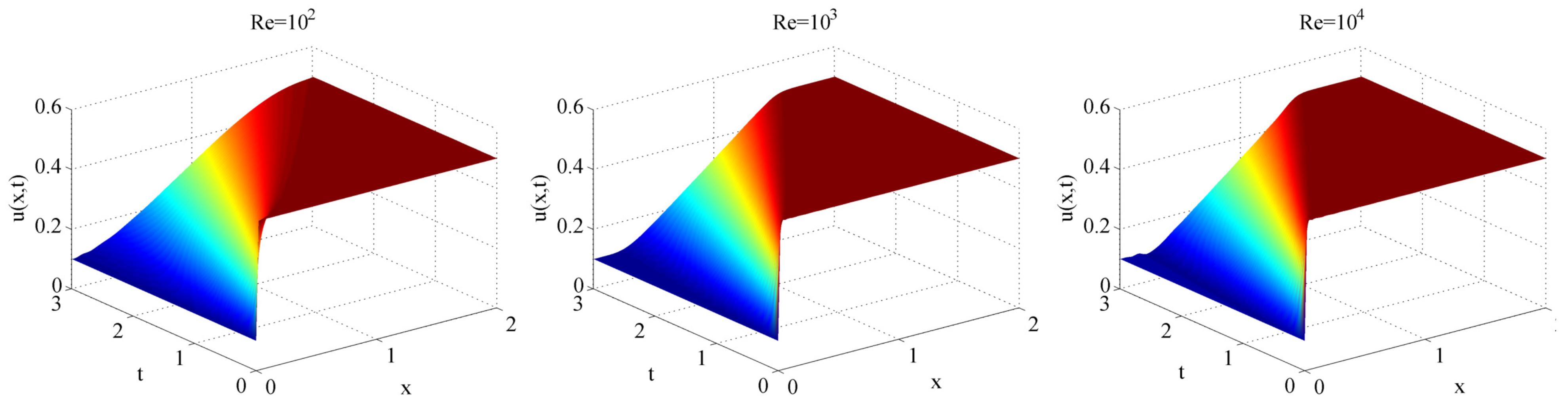
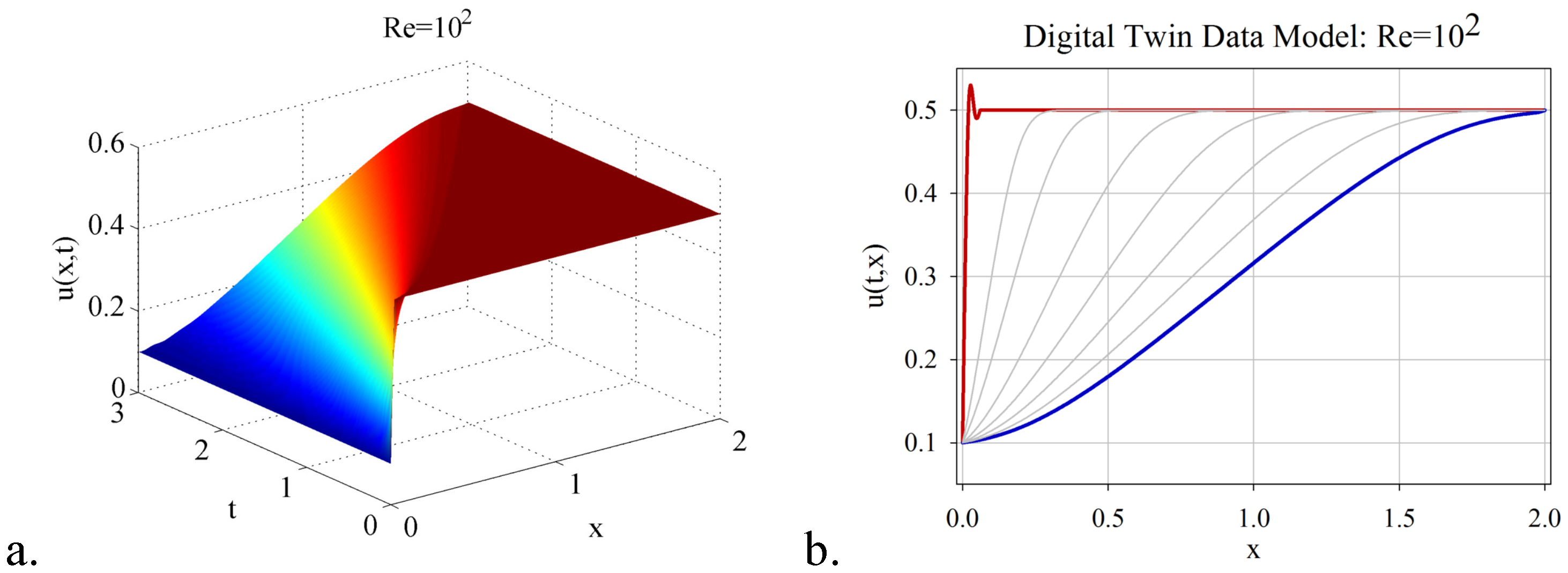
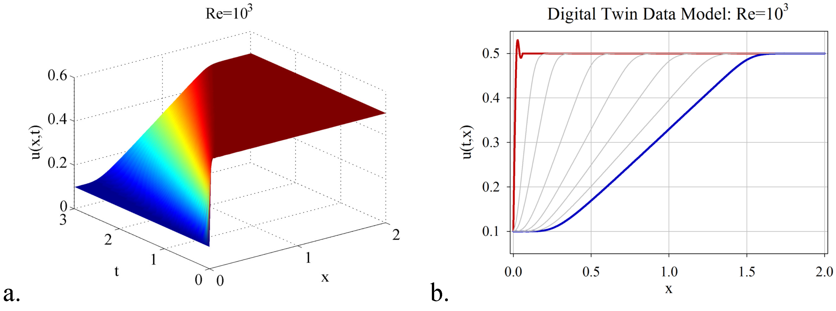
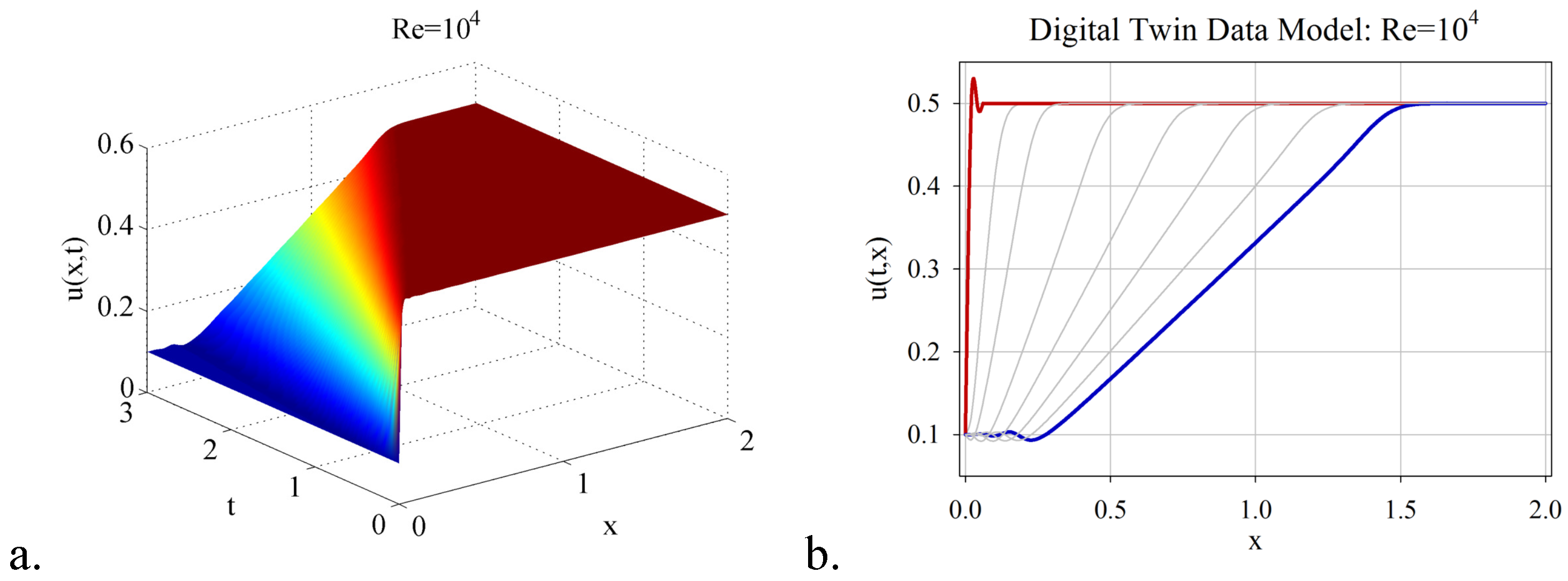
2. Shock Wave Phenomena: Full-Order Model of Nonlinear Viscous Burgers Equation

The non-intrusive experimental data are provided by the simulation of the nonlinear viscous Burgers equation model [44,45]:

$$\left\{\begin{array}{c}\frac{\partial }{\partial t}u\left(x,t\right)+\frac{\partial }{\partial x}\left(\frac{u{\left(x,t\right)}^2}{2}\right)=\nu \frac{{\partial }^2}{\partial x^2}u\left(x,t\right),x\in \left[0,L\right],t\in \left[0,T\right],\hfill \\ u\left(x,0\right)=u_0\left(x\right),\hfill \end{array}\right.$$

(1)

where $u\left(x,t\right)$ is the unknown function of time t, $\nu =1/Re$ is the viscosity term, and $Re$ is the Reynolds number. The discontinuous initial condition of the following form is considered:

$$u_0\left(x\right)=\left\{\begin{array}{c}{u}_L,x\le 0,\hfill \\ u_R,x>0.\hfill \end{array}\right.$$

(2)

This setting yields a shock wave phenomenon. The nonlinear evolution governed by the Burgers equation is obtained with the help of the Cole–Hopf transformation [46]. The Cole–Hopf transformation is defined by the following relation:

$$u=-2\nu \frac{1}{\phi }\frac{\partial \phi }{\partial x}.$$

(3)

Through an analytical handling we find that

$$\frac{\partial u}{\partial t}=\frac{2\nu }{{\phi }^2}\left(\frac{\partial \phi }{\partial t}\frac{\partial \phi }{\partial x}-\phi \frac{{\partial }^2\phi }{\partial x\partial t}\right),u\frac{\partial u}{\partial x}=\frac{4{\nu }^2}{{\phi }^3}\frac{\partial \phi }{\partial x}\left(\phi \frac{{\partial }^2\phi }{\partial x^2}-\frac{\partial \phi }{\partial x}\frac{\partial \phi }{\partial x}\right),$$

(4)

$$\nu \frac{{\partial }^{2}u}{\partial x^2}=-\frac{2{\nu }^2}{{\phi }^3}\left(2{\left(\frac{\partial \phi }{\partial x}\right)}^3-3\phi \frac{{\partial }^2\phi }{\partial x^2}\frac{\partial \phi }{\partial x}+{\phi }^2\frac{{\partial }^3\phi }{\partial x^3}\right).$$

(5)

Substituting these expressions into (1) it follows that

$$\frac{\partial \phi }{\partial x}\left(\frac{\partial \phi }{\partial t}-\nu \frac{{\partial }^2\phi }{\partial x^2}\right)=\phi \left(\frac{{\partial }^2\phi }{\partial x\partial t}-\nu \frac{{\partial }^3\phi }{\partial x^3}\right)=\phi \frac{\partial }{\partial x}\left(\frac{\partial \phi }{\partial t}-\nu \frac{{\partial }^2\phi }{\partial x^2}\right).$$

(6)

Relations (6) indicate that, if $\phi$ solves the heat equation, then $u\left(x,t\right)$ given by the Cole–Hopf transformation (3) solves the viscous Burgers Equation (1). Thus the viscous Burgers Equation (1) is reduced to the following one

$$\left\{\begin{array}{c}\frac{\partial \phi }{\partial t}-\nu \frac{{\partial }^2\phi }{\partial x^2}=0,x\in R,t>0,\nu >0,\hfill \\ \phi \left(x,0\right)={\phi }_0\left(x\right)=e^{-{\int }_0^x\frac{u_0\left(\xi \right)}{2\nu }d\xi },x\in \mathbb{R}.\hfill \end{array}\right.$$

(7)

Taking the Fourier transform with respect to x for both the heat equation and the initial condition (7) the analytic solution is obtained in the following form:

$$\phi \left(x,t\right)=\frac{1}{2\sqrt{\pi \nu t}}\underset{-\infty }{\overset{\infty }{\int }}{\phi }_0\left(\xi \right)e^{-\frac{{(x-\xi )}^2}{4\nu t}}d\xi .$$

(8)

From the Cole–Hopf transformation (3) the analytic solution to the problem (1) is returned in the following form:

$$u\left(x,t\right)=\frac{{\int }_{-\infty }^{\infty }\frac{x-\xi }{t}{\phi }_0\left(\xi \right)e^{-\frac{{\left(x-\xi \right)}^2}{4\nu t}}d\xi }{{\int }_{-\infty }^{\infty }{\phi }_0\left(\xi \right)e^{-\frac{{\left(x-\xi \right)}^2}{4\nu t}}d\xi }.$$

(9)

The constants used for the test model are:

$$L=2,T=3,u_L=0.1,u_R=0.5.$$

The training data comprises of

$N_t+1=301$ total number of snapshots taken in time at regularly spaced time intervals $\Delta t=0.01$,

$N_x=101$ number of spatial measurements per time snapshot.

Three solution types will be discussed in this paper, corresponding to Reynolds numbers of $\mathrm{Re}={10}^2$, $\mathrm{Re}={10}^3$, and $\mathrm{Re}={10}^4$, respectively (see Figure 1). The model solution exhibits some oscillations for all three experiments. The unphysical oscillation originates due to high Reynolds numbers. It is worth noticing that, when the Reynolds number increases, the numerical solution exhibits more oscillations, so that the fluid dynamics become more and more complex.

The aim of this paper is to identify a reduced order model of the nonlinear viscous Burgers equation model to approximate, as faithfully as possible, the true solution and to create a digital twin data model of low complexity for the three shock wave phenomena, respectively. An efficient numerical technique is provided in the following sections.

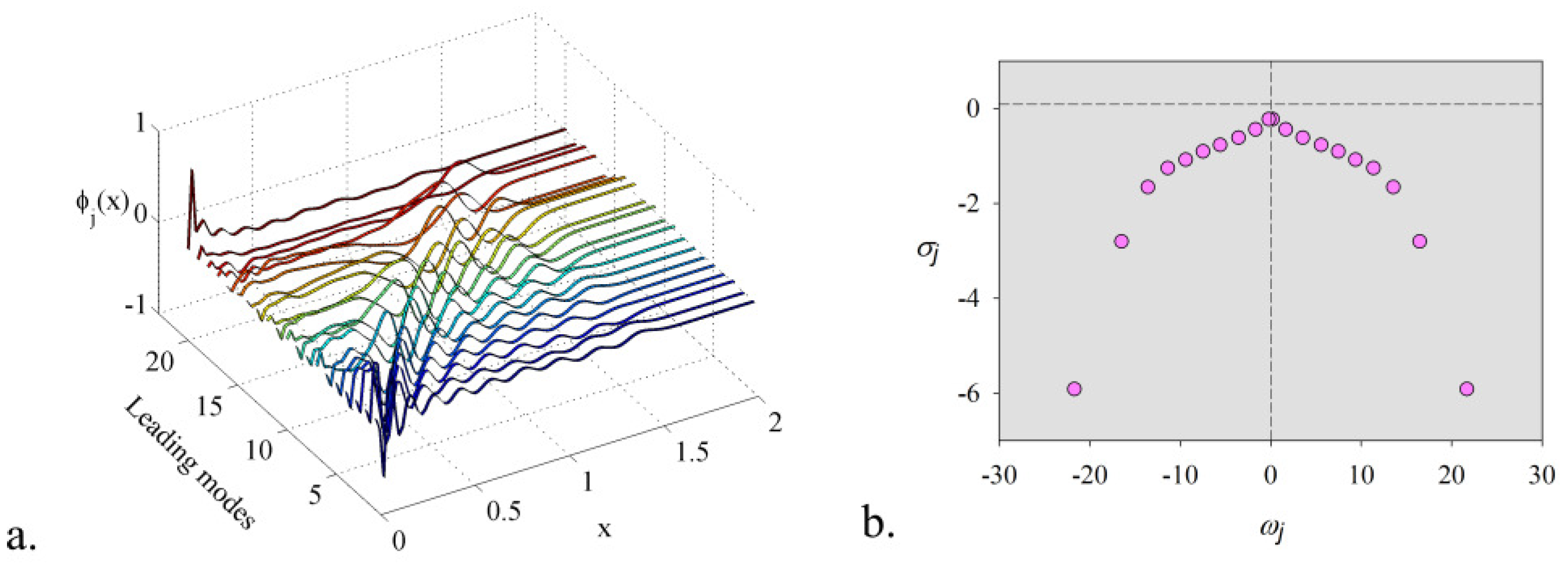
3. Reduced Order Modeling Based on Dynamic Mode Decomposition

The data $u_i\left(t,x\right)=u\left(t_i,x\right),t_i=i\Delta t,i=0,\dots ,N_t$ are collected at the constant sampling time $\Delta t$, x representing the spatial coordinate.

A data matrix whose columns represent the individual data samples, called the snapshot matrix, is constructed in the following manner:

$$V=\left[\begin{array}{cccc}{u}_0& u_1& \dots & u_{N_t}\end{array}\right]\in {\mathbb{R}}^{N_x\times (N_t+1)}.$$

(10)

Each column $u_i$ is a vector with $N_x$ components, representing the numerical measurements.

Following the Koopman decomposition assumption [19], we consider that a propagator matrix $\mathcal{A}$ exists that maps every column vector onto the next one:

$$\left\{u_0,u_1=\mathcal{A}{u}_0,u_2=\mathcal{A}{u}_1={\mathcal{A}}^2{u}_0,\dots ,u_{N_t}=\mathcal{A}{u}_{N_t-1}={\mathcal{A}}^{N_t}{u}_0\right\}.$$

(11)

In the next computational step, a matrix $V_0$ is formed with the first $N_t$ columns and the matrix $V_1$ contains the last $N_t$ columns of V:

$$V_0=\left[\begin{array}{cccc}{u}_0& u_1& \dots & u_{N_t-1}\end{array}\right]\in {\mathbb{R}}^{N_x\times N_t},V_1=\left[\begin{array}{cccc}{u}_1& u_2& \dots & u_{N_t}\end{array}\right]\in {\mathbb{R}}^{N_x\times N_t}.$$

(12)

For a sufficiently long sequence of the snapshots, let us suppose that the last snapshot $u_{N_t}$ can be written as a linear combination of previous $N_t$ vectors, such that

$$u_{N_t}=c_0{u}_0+c_1{u}_1+\dots +c_{N_t-1}{u}_{N_t-1}+\mathcal{R},$$

(13)

in which ${\mathrm{c}}_i\in \mathbb{R},\mathrm{i}=0,\dots ,{\mathrm{N}}_{\mathrm{t}}-1$ and $\mathcal{R}$ is the residual vector. The following relations are assembled:

$$\left\{u_1,u_2,\dots u_{N_t}\right\}=\mathcal{A}\left\{u_0,u_1,\dots u_{N_t-1}\right\}=\left\{u_1,u_2,\dots ,V_{0}c\right\}+\mathcal{R},$$

(14)

where $c={\left(\begin{array}{cccc}{c}_0& c_1& \dots & c_{N_t-1}\end{array}\right)}^T$ is the unknown column vector.

In matrix notation form, Equation (14) reads

$$\mathcal{A}{V}_0=V_0\mathcal{S}+\mathcal{R},\mathcal{S}=\left(\begin{array}{cccc}0& \dots & 0& c_0\\ 1& & 0& c_1\\ ⋮& ⋮& ⋮& ⋮\\ 0& \dots & 1& c_{N_t-1}\end{array}\right),$$

(15)

where $\mathcal{S}$ is the companion matrix.

Relation (15) is true when the residual

$$\mathcal{R}=u_{N_t}-V_{0}c,$$

(16)

is minimised when c is chosen such that $\mathcal{R}$ is orthogonal to $span\left\{u_0,\dots ,u_{N_t-1}\right\}$.

The goal of DMD algorithm is to solve the eigenvalue problem of the companion matrix $\mathcal{S}$

$$V_1=\mathcal{A}{V}_0=V_0\mathcal{S}+\mathcal{R},$$

(17)

where $\mathcal{S}$ approximates the eigenvalues of $\mathcal{A}$ when ${∥\mathcal{R}∥}_2\to 0$, which is equivalent to solving the minimisation problem

$$\underset{\mathcal{S}}{Minimize}\mathcal{R}={∥V_1-V_0\mathcal{S}∥}_2.$$

(18)

In the author’s previous work [18], the solution to the minimisation problem (18) is estimated by multiplying $V_1$ by the Moore–Penrose pseudoinverse [47] of $V_0$:

$$\mathcal{S}={\left(V_0\right)}^{+}{V}_1.$$

(19)

As it was previously pointed out in [18], the Moore–Penrose pseudoinverse approach might not be feasible when dealing with high dimensional data.

Following Schmid [48], who was the first to introduce the DMD as a numerical tool to compute the Koopman modes, we have developed an alternate algorithm based on Singular Value Decomposition (SVD) of snapshot matrix $V_0$. This approach is helpful especially when the matrix $V_0$ is rank deficient (${\mathrm{N}}_x>{\mathrm{N}}_t$). In the following, this technique will de described.

First, a singular value decomposition of $V_0$ is identified:

$$V_0=U\Sigma W^H,$$

(20)

where U contains the proper orthogonal modes of $V_0$, $\Sigma$ is a square diagonal matrix containing the singular values of $V_0$ and $W^H$ is the conjugate transpose of W.

The eigenvectors of $\mathcal{S}$ form a basis for the span of $\mathcal{A}$, therefore, every column vector is as a linear combination of the eigenvectors

$$u_i=\sum _{j=1}^{N_t}{\mathcal{A}}^{i-1}{\tilde{a}}_j{\varphi }_j\iff u_i=\sum _{j=1}^{N_t}{\tilde{a}}_j{\lambda }_j^{i-1}{\varphi }_j,i=1,\dots ,N_t.$$

(21)

As a consequence of (21), the data snapshots at every time step $\left\{{\mathrm{t}}_1,\dots ,{\mathrm{t}}_{N_t}\right\}$ are a linear combination of DMD modes according to

$$\begin{array}{c}{V}_1=\left[\begin{array}{cccc}{u}_1& u_2& \dots & u_{N_t}\end{array}\right]\hfill \\ =\left[\begin{array}{cccc}{\varphi }_1& {\varphi }_2& \dots & {\varphi }_{N_t}\end{array}\right]\left(\begin{array}{cccc}{\tilde{a}}_1& & & \\ & {\tilde{a}}_2& & \\ & & ⋮& \\ & & & {\tilde{a}}_{N_t}\end{array}\right)\left(\begin{array}{ccccc}1& {\lambda }_1^1& {\lambda }_1^2& \dots & {\lambda }_1^{N_t-1}\\ 1& {\lambda }_2^1& {\lambda }_2^2& \dots & {\lambda }_2^{N_t-1}\\ 1& ⋮& ⋮& ⋮& ⋮\\ ⋮& ⋮& ⋮& ⋮& ⋮\\ 1& {\lambda }_{N_t}^1& {\lambda }_{N_t}^2& \dots & {\lambda }_{N_t}^{N_t-1}\end{array}\right)\hfill \end{array},$$

(22)

where the right eigenvectors of $\mathcal{S}$, ${\varphi }_j\in \mathbb{C}$ are dynamic shape (or Koopman) modes, the eigenvalues of $\mathcal{S}$, ${\lambda }_j$ are called Ritz values [49], and the coefficients ${\tilde{a}}_j\in \mathbb{C}$ are denoted as amplitudes or Koopman eigenfunctions. Each Ritz value ${\lambda }_j=e^{\left({\sigma }_j+i{\omega }_j\right)\Delta t}$ is associated with the growth rate ${\sigma }_j$ and the frequency ${\omega }_j$.

The superposition of all Koopman modes, weighted by their amplitudes and frequencies, approximates the entire data sequence, but there are also modes that have a weak contribution; therefore these modes can be eliminated. The goal of the algorithm is to produce the ROM involving only the most significant modes, having a strong contribution to the data representation, which are called in the following the leading modes.

The data snapshots at every time step $\left\{{\mathrm{t}}_1,\dots ,{\mathrm{t}}_{N_t}\right\}$ are represented as a linear combination of the leading modes according to the following relation:

$$u_{DMD}\left(t_i,x\right)=\sum _{j=1}^{N_{DMD}}{\tilde{a}}_j{\varphi }_j\left(x\right){\lambda }_j^{i-1},i\in \left\{1,\dots ,N_t\right\},t_i\in \left\{{\mathrm{t}}_1,\dots ,{\mathrm{t}}_{N_t}\right\},$$

(23)

where $N_{DMD}$ represents the number of leading modes involved in reconstruction of data snapshots.

One advantage of DMD is that each mode is associated with a pulsation, a growth rate, and each mode oscillates at a single frequency, as seen from (23). Representation (23) is suitable when one wants to isolate a mode with a certain frequency, to identify a maximum or a minimum amplitude, and for hydrodynamic stability analysis also. In the seminal article [36], Mezić provides a characterisation of Koopman modes in the Banach space using Generalised Laplace Analysis.

For the purpose of model order reduction, in the present paper the following form is utilised:

$$u_{DMD}\left(t_i,x\right)=\sum _{j=1}^{N_{DMD}}{a}_j\left(t_i\right){\varphi }_j\left(x\right),t_i\in \left\{{\mathrm{t}}_1,\dots ,{\mathrm{t}}_{N_t}\right\},$$

(24)

where ${\varphi }_j\in \mathbb{C}$ are dynamic leading modes and $a_j\left(t_i\right)={\tilde{a}}_j{\lambda }_j^{i-1},$$i\in \left\{1,\dots ,N_t\right\},$$j\in \left\{1,\dots ,N_{DMD}\right\}$ are modal amplitudes.

It is worth noticing that the $N_{DMD}$ leading modes involved in ROM representation (24) are not the first $N_{DMD}$ modes from representation (22). The leading modes represent a subset of DMD modes that will be selected from all computed DMD modes via numerical algorithm presented in the next section.

4. Offline Stage: Randomized Dynamic Mode Decomposition

The process of calculating a reduced order model consists of two steps. In the first step the spatial components of the model are calculated. These are the so-called modes. These functions do not depend on time but only on the spatial component, which is why this stage is called the offline stage. Moreover, the calculation step of the modes is performed only once. The model is not complete without the temporal component, i.e., the temporal coefficients of the reduced order model. These are calculated in the second step, when the mathematical model has to be integrated over time. Furthermore, if desired, one can calculate the dynamics of the reduced order model at a given point in time. That is why this second step is called the online stage, which can be performed whenever one wants to simulate the behaviour of the initial process.

The modes’ selection plays a central role in model reduction and also constitutes the source of many discussions among modal decomposition practitioners [21,23,50,51]. Several procedures for selecting the most influential modes in dynamic mode decomposition can be found in the author’s previous papers [15,18,52]. The procedure of randomisation of data prior to singular value decomposition (SVD) was first introduced in [30] for image processing and in [31] with application to fluid dynamics. The DMD algorithm was combined with a randomized SVD function, aiming to improve the accuracy of the reduced order linear model and to reduce the CPU time. The major advantage of this method is that it does not require an additional selection algorithm of the DMD modes. The randomized DMD produces a reduced order subspace of Ritz values, having the same dimension as the rank of randomized SVD function, where the leading modes reside. Recently, the author successfully applied the technique of adaptive randomized DMD in epidemiology [53,54].

The objective of the DMD-based ROM is to represent, as accurately as possible, a high fidelity solution using the dynamics given by the DMD modes. It is then natural to seek the leading DMD modes and their temporal eigenfunctions that minimise the error between the raw data and the reduced order model:

$$E_{DMD}={〈{∥u\left(x,t\right)-u_{DMD}\left(x,t\right)∥}_2〉}_T,$$

(25)

where ${〈·〉}_T$ is a time average operator over $\left[t_1,T\right]$ and ${∥·∥}_2$ is the $L_2$-norm of ${\mathbb{R}}^{N_x}$. In this paper, ${〈·〉}_T$ corresponds to the arithmetic time-average on $N_t$ equally spaced elements of the interval $\left[t_1,T\right]$:

$${〈f\left(t\right)〉}_T=\frac{1}{N_t}\sum _{i=1}^{N_t}f\left(t_i\right),t_i\in \left\{t_1,t_2,\dots ,t_{N_t}=T\right\}.$$

(26)

Determination of the optimal rank of the ROM, of the leading modes, and associated temporal coefficients then amounts to finding the solution to the following optimisation problem:

$$\begin{array}{c}\underset{{\varphi }_j,a_j}{Find}{u}_{DMD}\left(t_i,x\right)={\displaystyle \sum _{j=1}^{N_{DMD}}}{a}_j\left(t_i\right){\varphi }_j\left(x\right),t_i\in \left\{{\mathrm{t}}_1,\dots ,{\mathrm{t}}_{N_t}\right\},\hfill \\ Subjectto{N}_{DMD}=argmin\left\{E_{DMD}\right\},N_{DMD}\in \mathbb{N},N_{DMD}\ge 2,\hfill \end{array}$$

(27)

where $E_{DMD}$ is the error of the low-rank model defined by Equation (25).

This paper presents an improved version of randomized dynamic mode decomposition introduced in [31], augmented with the modern tool of deep learning artificial intelligence. In the following, Algorithm 1 describes the randomized dynamic mode decomposition. Algorithm 2 describes the routine used to produce the randomized singular value decomposition.

Algorithm 1: Randomized Dynamic Mode Decomposition

Initial data:$V_0\in {\mathbb{R}}^{N_x\times N_t}$, $V_1\in {\mathbb{R}}^{N_x\times N_t}$, integer target rank $k\ge 2$ and $k<N_t$. For $k=2$ to $N_t-1$. Produce the randomized singular value decomposition of rank k $\left[U,\Sigma ,W\right]=k-\mathbf{RSVD}\left(V_0,k\right),$ where U contains the proper orthogonal modes of $V_0$ and $\Sigma$ contains the singular values. The RSVD function is described in continuation of this algorithm. Solve the minimisation problem (18). Compute dynamic modes solving the eigenvalue problem $SX=X\mathsf{\Lambda }$ and obtain dynamic modes as $\mathsf{\Phi }=UX$. The diagonal entries of $\mathsf{\Lambda }$ represent the eigenvalues $\lambda$. Project dynamic modes onto the first snapshot to calculate the vector containing dynamic modes amplitudes $Ampl={\left(a_j\right)}_{j=1}^{rank\left(\mathsf{\Lambda }\right)}$. The DMD model of rank k is given by the product $$V_{DMD}=\mathsf{\Phi }·diag\left(Ampl\right)·Van,$$ (28) where the Vandermonde matrix is $$Van=\left(\begin{array}{ccccc}1& {\lambda }_1^1& {\lambda }_1^2& \dots & {\lambda }_1^{N_t-1}\\ 1& {\lambda }_2^1& {\lambda }_2^2& \dots & {\lambda }_2^{N_t-1}\\ 1& ⋮& ⋮& ⋮& ⋮\\ \dots & \dots & \dots & \dots & \dots \\ 1& {\lambda }_k^1& {\lambda }_k^2& \dots & {\lambda }_k^{N_t-1}\end{array}\right).$$ Solve the optimisation problem (27) and obtain the optimal low rank k and associated $V_{DMD}$. Output:k, $V_{DMD}$.

The following routine is used to produce the randomized singular value decomposition.

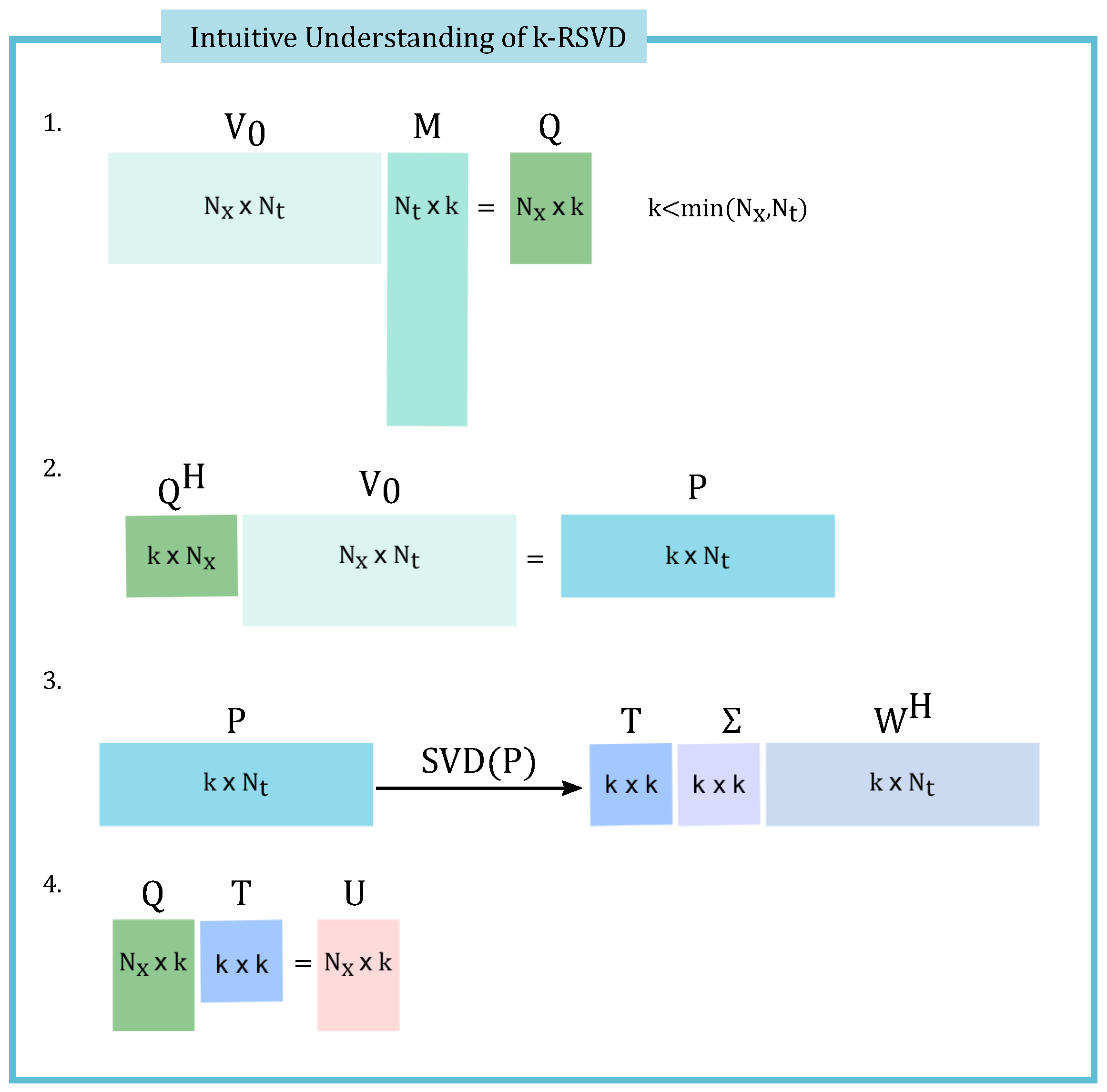
Algorithm 2: Randomized Singular Value Decomposition of Rank k (k-RSVD)

Initial data:$V_0\in {\mathbb{R}}^{N_x\times N_t}$, integer target rank $k\ge 2$ and $k<N_t$. Generate random test matrix $M=rand\left(N_t,r\right)$, $r=min\left(N_t,2k\right)$. Compute sampling matrix by multiplication of snapshot matrix with random matrix $Q=V_{0}M$. Orthonormalisation of sampling matrix via Gram–Schmidt orthonormal method $Q\leftarrow GramSchmidt\left(Q\right)$. Projection of snapshot matrix to smaller space $V=Q^H{V}_0$, where H denotes the conjugate transpose. Produce the economy-size singular value decomposition of low-dimensional snapshot matrix $\left[T,\Sigma ,W\right]=SVD\left(V\right)$. Compute the right singular vectors $U=QT$. Output: Procedure returns $U\in {\mathbb{R}}^{N_x\times k}$, $\Sigma \in {\mathbb{R}}^{k\times k}$, $W\in {\mathbb{R}}^{N_t\times k}$.

An intuitive understanding of k-RSVD is illustrated in Figure 2. By using the randomized singular value decomposition (RSVD) technique the problem dimension is reduced. Thus, a computationally expensive algorithm is avoided.

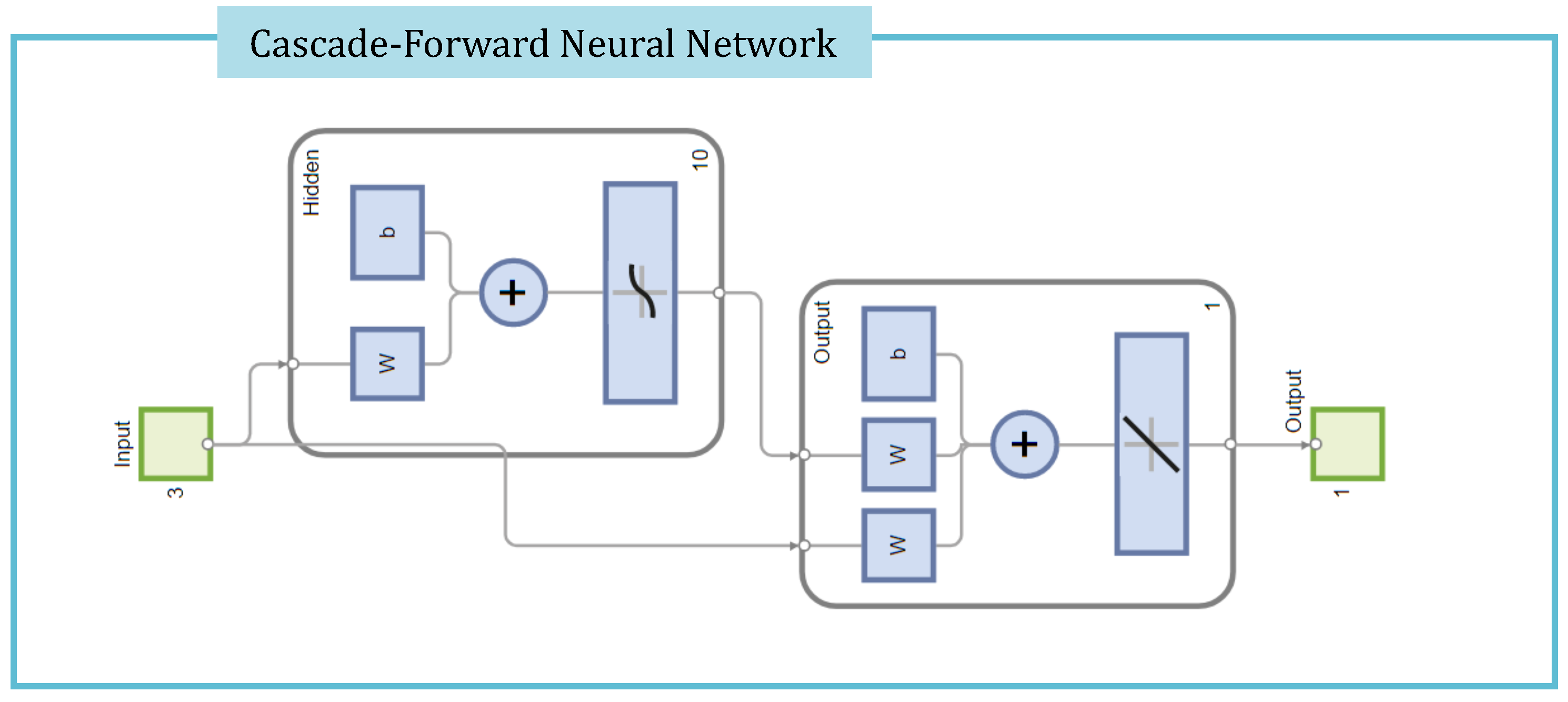
5. Online Stage: Fast Digital Twin Data Model Identification Using Deep Learning Nonlinear Autoregressive Estimators

The algorithm previously described allows the identification of the leading dynamic modes and their associated temporal coefficients in discrete form. The goal in this section is the identification of the reduced order digital twin data model (DTM) in continuous form:

$$u_{DTM}^{ROM}\left(t,x\right)=\sum _{j=1}^{N_{DMD}}{\widehat{a}}_j\left(t\right){\varphi }_j\left(x\right),t\in \left[0,T\right],$$

(29)

where ${\varphi }_j$, $j=1,\dots ,N_{DMD}$ are the DMD modes and ${\widehat{a}}_j\left(t\right)$, $j=1,\dots ,N_{DMD}$ represent the temporal coefficients of the DTM.

Nonlinear AutoRegressive models with eXogenous inputs (NLARX) represent a novel approach in the field of nonlinear system identification [55,56,57]. Since the emergence of artificial neural networks as numerical tools, NLARX models have been used for various purposes, ranging from simulation [58], to nonlinear predictive control [59] or higher order nonlinear optimisation problems [60,61,62,63].

In this paper the application of NLARX models is investigated to a high-fidelity approximation of temporal coefficients of the DMD-ROM model (29). Let $a\left(t\right)$ be the system input represented by the DMD computed amplitudes at discrete time instances $t\in \left\{{\mathrm{t}}_1,\dots ,{\mathrm{t}}_{N_t}\right\}$ and $\widehat{a}\left(t\right)$ be the output.

The formulation of the NLARX model is described in the following manner:

$$\widehat{a}\left(t\right)=f\left[\widehat{a}\left(t-1\right),\dots ,\widehat{a}\left(t-n_a\right),a\left(t-n_k\right),\dots ,a\left(t-n_k-n_b+1\right)\right]+e\left(t\right),$$

(30)

where the $n_a$ is the integer number of past output terms, $n_b$ is the number of past input terms used to predict the current output, $n_k$ is the pure input delay, f is a nonlinear function implemented by an artificial neural network and $e\left(t\right)$ represents the modeling error. The NLARX model output represents a function of regressors that are transformations of past inputs and past outputs. This function is consisting from a linear block and a nonlinear block. The model output is the sum of the outputs of the two blocks.

The NLARX training model can be cast as a non-linear unconstrained optimisation problem of the following form:

$$\theta \left(n_a,n_b,n_k\right)=argmin\frac{1}{2N_t}\sum _{i=1}^{N_t}{∥a\left(t_i\right)-\widehat{a}\left(t_i\right)∥}_2,$$

(31)

where the training set consists of the measured input $a\left(t\right)$, $\widehat{a}\left(t\right)$ is the NLARX output, ${∥·∥}_2$ is the $L_2$ norm, and $\theta \left(n_a,n_b,n_k\right)$ represents the parameter vector of the nonlinear function f.

One of the most important aspects of an application of a NLARX network is a proper selection of inputs, input delays, and output delays. The presented algorithm modifies the network parameters $\theta \left(n_a,n_b,n_k\right)$ over the complete trajectory to achieve the minimal value of (31). The nonlinear estimator f is implemented in the form of a cascade forward neural network with 10 hidden layer sizes; see Figure 3.

In the next section, the numerical results will be detailed.

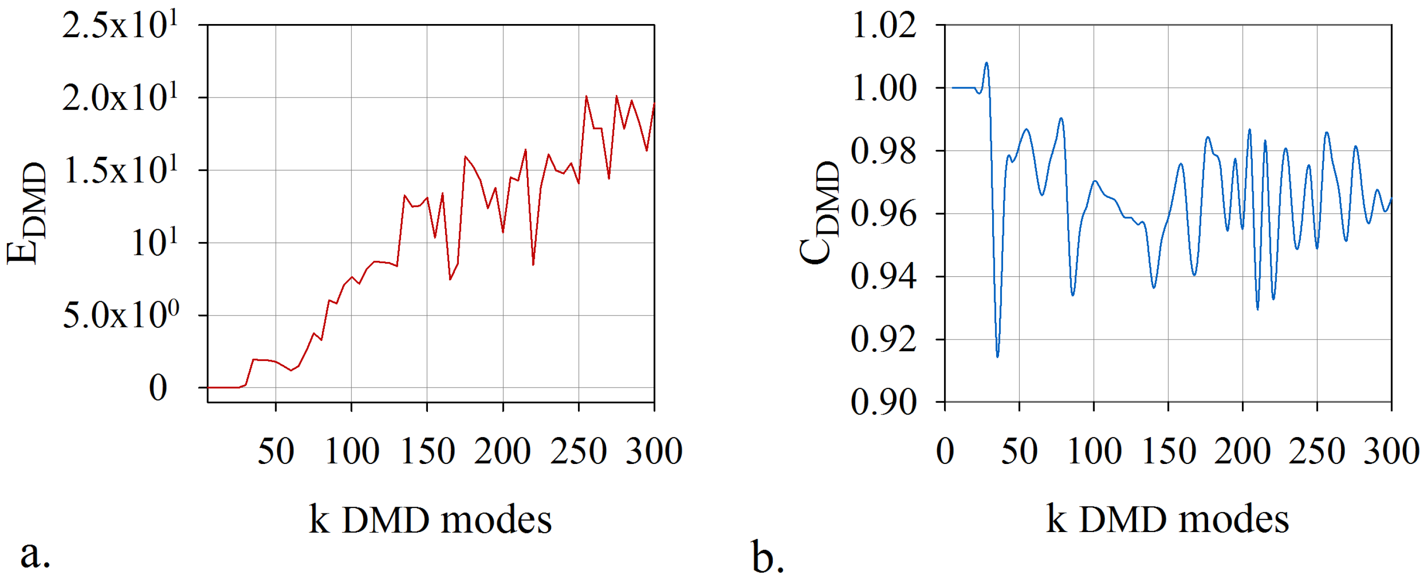
6. Numerical Results: Computational Efficiency of the Algorithm

In the following, the numerical results are presented. The viscous Burgers equation models (1) and (2) were used to generate three shock wave phenomena with increasing complexity. The optimal rank of the reduced DMD model is obtained as the unique solution to the optimisation problem (27), which has been solved by a simulated annealing algorithm [64,65].

A major advantage that comes from the application of a randomized DMD algorithm is that it leads to the optimal low rank $N_{DMD}$ and associated DMD subspace where the most influential DMD modes are identified.

The correlation coefficient defined below is used as additional metric to validate the quality of the low-rank DMD model:

$$C_{DMD}=\frac{{{〈{∥u\left(x,t\right)·u_{DMD}\left(x,t\right)∥}_2〉}_T}^2}{{〈{∥u{\left(x,t\right)}^H·u\left(x,t\right)∥}_2〉}_T{〈{∥u_{DMD}{\left(x,t\right)}^H·u_{DMD}\left(x,t\right)∥}_2〉}_T},$$

(32)

where $u\left(t,x\right)$ means the numerical data, $u_{DMD}\left(t,x\right)$ represent the computed solution by means of the reduced order DMD model, $\left(·\right)$ represents the Hermitian inner product, H denotes the conjugate transpose, and ${〈·〉}_T$ is the norm defined by Equation (26).

Figure 4, Figure 5 and Figure 6 present the process of evaluation of DMD model target rank. The error and the correlation coefficient computed as a function of retained number of dynamic modes are presented, respectively, in the cases $Re={10}^2$, $Re={10}^3$, and $Re={10}^4$, for up to 300 modes. It is obvious that increasing the number of modes leads neither to error reduction nor to improved correlation. On the contrary, working with too many modes can worsen the performance of the reduced order model. The algorithm proposed in this article achieves two remarkable things. The algorithm determines the minimum number of modes (or the order of DMD subspace) required for the low-order model to have the required performances, i.e., minimum error and maximum correlation with the initial data, respectively. At the same time, the algorithm selects the modes that have the maximum influence and that will contribute to the calculation of the reduced order model.

Table 1. Comparison of the numerical results returned by the randomized dynamic mode decomposition algorithm. A total of 300 data snapshots have been processed.

Test Case	Model Rank	Error	Correlation Coefficient
$Re={10}^2$	$N_{DMD}=15$	$E_{DMD}=3.1984\times 10^{-7}$	$C_{DMD}=1.0000$
$Re={10}^3$	$N_{DMD}=20$	$E_{DMD}=4.4247\times 10^{-7}$	$C_{DMD}=1.0000$
$Re={10}^4$	$N_{DMD}=20$	$E_{DMD}=5.4416\times 10^{-8}$	$C_{DMD}=1.0000$

presents the order of DMD subspace obtained in the three test cases, next to the error defined by Equation (25) and the correlation coefficient defined by Equation (32).

The algorithm introduced in this paper confers the best correlation coefficient to the DMD model (see Table 1); thus, a digital twin data model was identified. The DMD leading modes are illustrated in Figure 7, Figure 8 and Figure 9, next to the representation of the modal growth rates and the associated frequencies of the eigenvectors of the Koopman matrix $\mathcal{S}$ for the three test cases, respectively.

The coefficients ${\widehat{a}}_j\left(t\right)$, $j=1,\dots ,N_{DMD}$ of the reduced order model (29) have been estimated for the entire time window by considering the DMD computed coefficients as inputs of the NLARX model (30). The numbers of the input terms, output terms and the value of delay are presented in

Table 2. Initial data for NLARX estimator of temporal coefficients, case of $Re={10}^2$, $N_{DMD}=15$.

Index	Outputs, Inputs, Delay	DTM Error and Correlation Coefficient
$j=1,$ 3–12, 14	$n_a=1,n_b=2,n_k=1$	$E_{DTM}=8.0806\times {10}^{-4}$
$j=2$	$n_a=2,n_b=2,n_k=2$	$C_{DTM}=1.0000$
$j=13,15$	$n_a=1,n_b=1,n_k=1$

,

Table 3. Initial data for NLARX estimator of temporal coefficients, case of $Re={10}^3$, $N_{DMD}=20$.

Index	Outputs, Inputs, Delay	DTM Error and Correlation Coefficient
$j=1,4,$ 10–12	$n_a=2,n_b=1,n_k=1$	$E_{DTM}=1.3080\times {10}^{-4}$
$j=2,3,13$	$n_a=1,n_b=1,n_k=2$	$C_{DTM}=1.0000$
j = 5–9	$n_a=1,n_b=1,n_k=5$
j = 14–19	$n_a=2,n_b=1,n_k=2$
$j=20$	$n_a=1,n_b=1,n_k=1$

and

Table 4. Initial data for NLARX estimator of temporal coefficients, case of $Re={10}^4$, $N_{DMD}=20$.

Index	Outputs, Inputs, Delay	DTM Error and Correlation Coefficient
$j=1,3,4,7$	$n_a=1,n_b=3,n_k=2$	$E_{DTM}=1.4000\times {10}^{-4}$
$j=2,5,6,8,$ 16–20	$n_a=1,n_b=2,n_k=2$	$C_{DTM}=1.0000$
$j=$ 9–15	$n_a=1,n_b=1,n_k=1$

, for the three test cases, respectively.

The following metrics have been used to perform a qualitative analysis of the digital twin data models (DTMs):

$$E_{DTM}={〈{∥u\left(x,t\right)-u_{DTM}^{ROM}\left(x,t\right)∥}_2〉}_T,$$

(33)

$$C_{DTM}=\frac{{{〈{∥u\left(x,t\right)·u_{DTM}^{ROM}\left(x,t\right)∥}_2〉}_T}^2}{{〈{∥u{\left(x,t\right)}^H·u\left(x,t\right)∥}_2〉}_T{〈{∥u_{DTM}^{ROM}{\left(x,t\right)}^H·u_{DTM}^{ROM}\left(x,t\right)∥}_2〉}_T},$$

(34)

where $E_{DTM}$ measures the error of the digital twin data model, $C_{DTM}$ is the correlation coefficient of the digital twin data model, $u\left(t,x\right)$ means the numerical data, $u_{DTM}^{ROM}\left(t,x\right)$ represent the computed solution by means of the DMD-ROM model, $\left(·\right)$ represents the Hermitian inner product, H denotes the conjugate transpose, and ${〈·〉}_T$ is the norm defined by Equation (26).

The very good correlation coefficients and the low values of errors presented in Table 2, Table 3 and Table 4 confirm the computational efficiency of the digital twin data models.

Solutions of the digital twin data models are illustrated in Figure 10, Figure 11 and Figure 12 for the three test cases, respectively.

The CPU time required in the offline-online stage is presented in Figure 13, for the three test cases.

The randomisation of input data has been leveraged to accelerate the computations. The required offline CPU time does not exceed two seconds and does not present large variations depending on the case study. The online CPU time falls between 8 and 17 s, depending on the index of the temporal coefficient which is estimated along the entire time window. It is obvious that the NLARX estimator requires more time to estimate the temporal behaviour in the case of very high Reynolds number.

Figure 14, Figure 15 and Figure 16 illustrate the validation for the first temporal coefficient, as simulated response of the optimal NLARX estimator, in the case of the three experiments, respectively. The dots represent the discrete data for the training of the neural network, while the line represents the continuous model of the temporal coefficient determined by the NLARX model network.

7. Conclusions

The present investigation has focused on the identification of high-fidelity digital twin data models from numerical code outputs by non-intrusive techniques (i.e., not requiring Galerkin projection of the governing equations onto the reduced modes basis). In this paper the author defined the concept of the digital twin data model (DTM) as a model of reduced complexity that has the main feature of mirroring the original process behaviour.

A new algorithm was developend that utilises a variant of the adaptive randomized dynamic mode decomposition introduced in [31] to obtain a reduced basis in the offline stage, combined with neural network based nonlinear autoregressive estimators in the online stage. The major advantages of the algorithm proposed in this work are the following:

• This method overcomes the inconveniences of developing and implementing a mode selection criterion associated with dynamic mode decomposition. The proposed technique does not require an additional selection algorithm of the DMD modes. The rank of the model, the leading modes, and the temporal coefficients have been determined by coupling the randomized dynamic mode decomposition with an optimisation problem whose constraint consists in the smallest error of digital twin model. A fast and accurate algorithm was produced, which provided the lowest rank for the model and the leading modes with the most significant contribution.
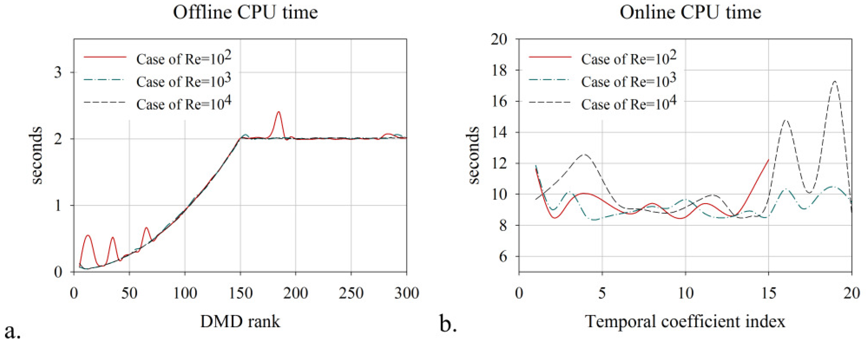
• A significant reduction of the offline-online CPU time was achieved, which confirms the feasibility of the algorithm.
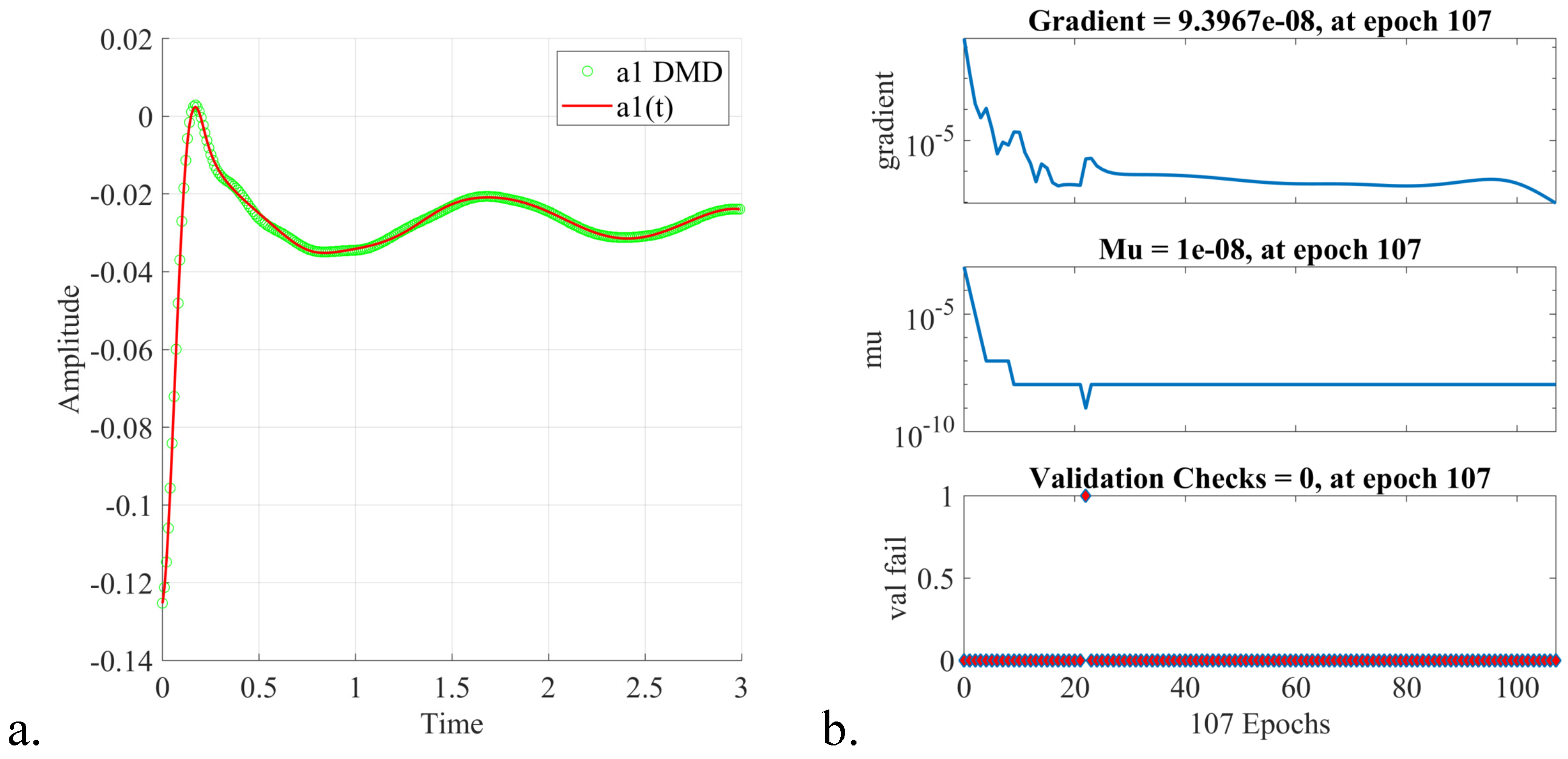
• Combining the randomized DMD with deep learning artificial intelligence, a digital twin data model for estimating the flow behaviour in the real-time window was derived. The DTM has been investigated in the numerical simulation of three shock wave phenomena with increasing complexity, with Reynolds number varying from ${10}^2$ to ${10}^4$. It was demonstrated that the significant advantage of DTM is to map the dynamics with high accuracy and reduced costs in CPU time and hardware, even to settings difficult to explore because of the rapidly changing dynamics over time (e.g., high Reynolds numbers).
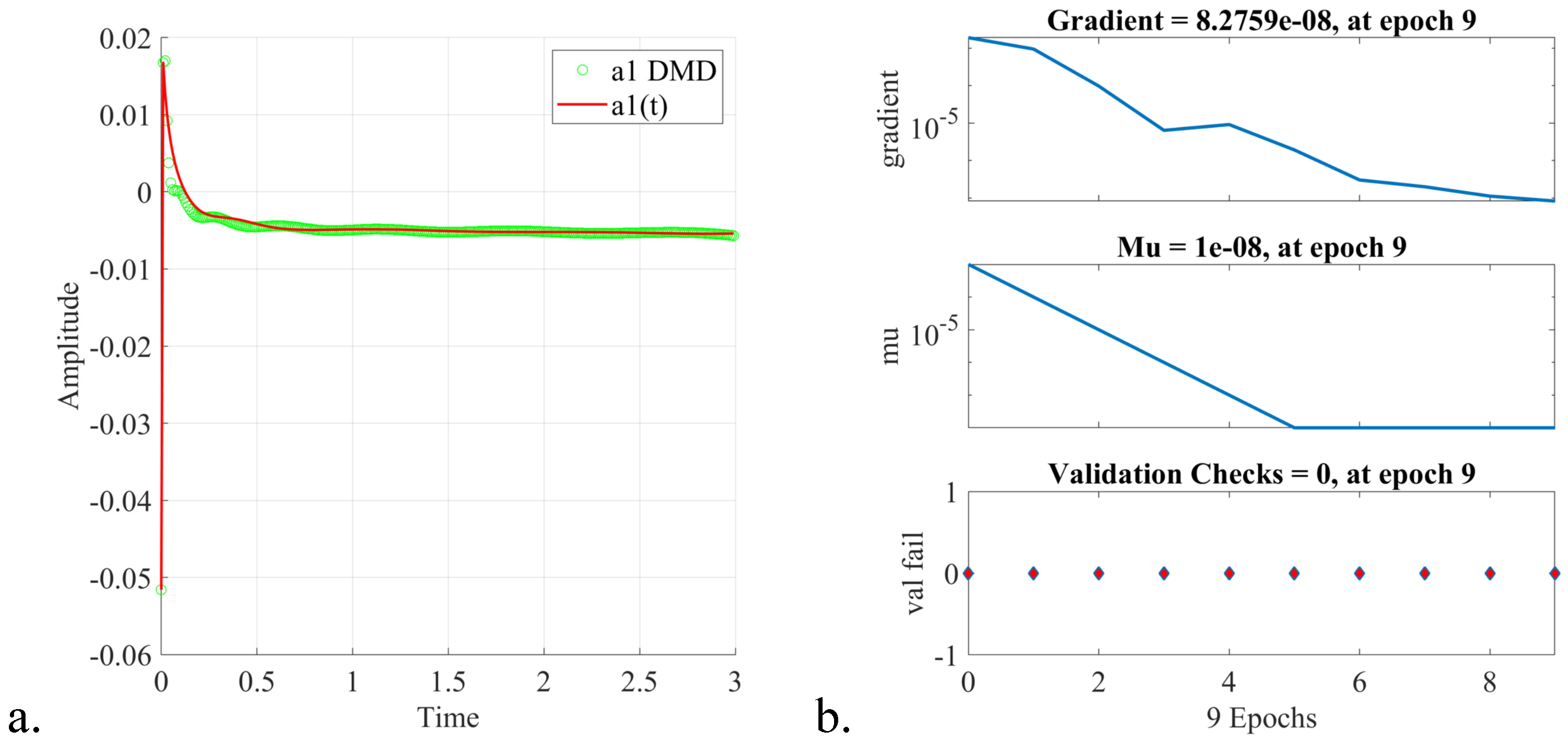
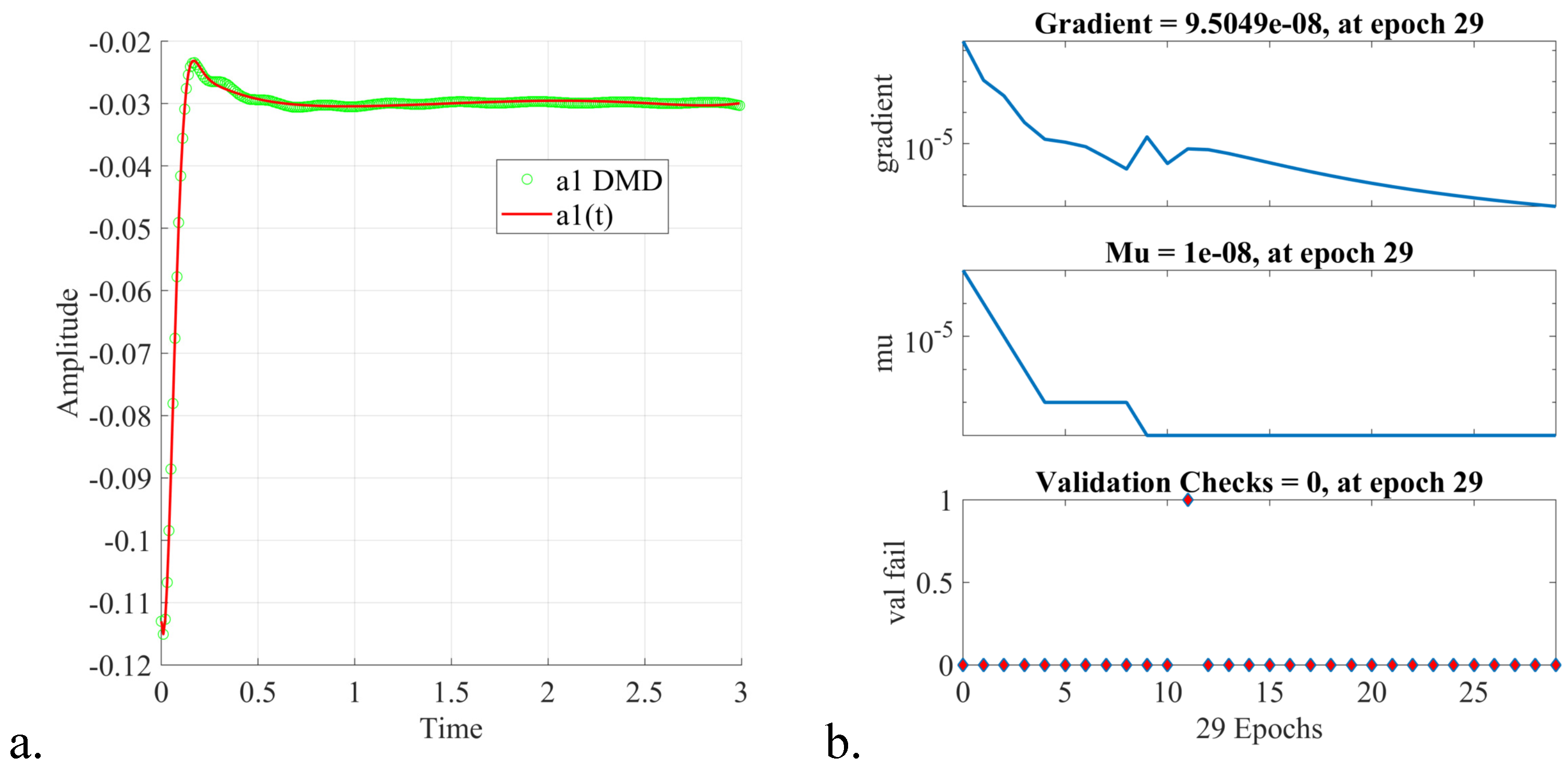
• The procedure of online estimation of the DTM temporal coefficients by employing deep learning nonlinear autoregressive estimators led to a fast and accurate identification of the digital twin data models. The computational efficiency of the proposed algorithm was thoroughly investigated, and a qualitative analysis of the DTM was provided in the three shock wave experiments.

There are a number of interesting directions that arise from this work. First, it will be a natural extension to apply the proposed algorithm to high-dimensional data originating from fluid dynamics and atmospheric measurements. The methodology presented here offers the main advantage of deriving faithful digital twin data models capable of providing a variety of information describing the real-time behaviour of the flow field. A future extension of this research will address an efficient numerical approach for modal decomposition of swirling flows, where the full mathematical model implies more sophisticated relations at domain boundaries that must be satisfied by the digital twin data model also.

References

1. Kim, N.H.; Sankar, B.V.; Kumar, A.V. Introduction to Finite Element Analysis and Design; John Wiley & Sons: Hoboken, NJ, USA, 2018. [Google Scholar]
2. Codina, R.; Badia, S.; Baiges, J.; Principe, J. Encyclopedia of Computational Mechanics; Chapter Variational Multiscale Methods in Computational Fluid Dynamics; John Wiley & Sons: Hoboken, NJ, USA, 2017. [Google Scholar]
3. Xiao, D.; Heaney, C.E.; Fang, F.; Mottet, L.; Hu, R.; Bistrian, D.A.; Aristodemou, D.; Navon, I.M.; Pain, C.C. A domain decomposition non-intrusive reduced order model for turbulent flows. Comput. Fluids 2019, 182, 15–27. [Google Scholar] [CrossRef] [Green Version]
4. Xiao, D.; Heaney, C.E.; Mottet, L.; Fang, F.; Lin, W.; Navon, I.M.; Guo, Y.; Matar, O.K.; Robins, A.G.; Pain, C.C. A reduced order model for turbulent flows in the urban environment using machine learning. Build. Environ. 2019, 148, 323–337. [Google Scholar] [CrossRef] [Green Version]
5. Dimitriu, G.; Stefanescu, R.; Navon, I.M. POD-DEIM approach on dimension reduction of a multi-species host-parasitoid system. Ann. Acad. Rom. Sci. Ser. Math. Appl. 2015, 7, 173–188. [Google Scholar]
6. Dumon, A.; Allery, C.; Ammar, A. Proper Generalized Decomposition method for incompressible Navier-Stokes equations with a spectral discretization. Appl. Math. Comput. 2013, 219, 8145–8162. [Google Scholar] [CrossRef] [Green Version]
7. Stefanescu, R.; Navon, I.M. POD/DEIM nonlinear model order reduction of an ADI implicit shallow water equations model. J. Comput. Phys. 2013, 237, 95–114. [Google Scholar] [CrossRef] [Green Version]
8. Wang, Z.; Akhtar, I.; Borggaard, J.; Iliescu, T. Proper orthogonal decomposition closure models for turbulent flows: A numerical comparison. Comput. Methods Appl. Mech. Eng. 2012, 10, 237–240. [Google Scholar] [CrossRef] [Green Version]
9. Muralidhar, N.K.B.; Rauter, N.; Mikhaylenko, A.; Lammering, R.; Lorenz, D.A. Parametric model order reduction of guided ultrasonic wave propagation in fiber metal laminates with damage. Modelling 2021, 2, 591–608. [Google Scholar] [CrossRef]
10. Mezic, I. Spectral properties of dynamical systems, model reduction and decompositions. Nonlinear Dyn. 2005, 41, 309–325. [Google Scholar] [CrossRef]
11. Rowley, C.W.; Mezic, I.; Bagheri, S.; Schlatter, P.; Henningson, D.S. Reduced-order models for flow control: Balanced models and Koopman modes. In Proceedings of the Seventh IUTAM Symposium on Laminar-Turbulent Transition, IUTAM Bookseries. Stockholm, Sweden, 1 December 2009; Volume 18, pp. 43–50. [Google Scholar]
12. Bagheri, S. Koopman-mode decomposition of the cylinder wake. J. Fluid Mech. 2013, 726, 596–623. [Google Scholar] [CrossRef]
13. Schmid, P.J.; Violato, D.; Scarano, F. Decomposition of Time-Resolved Tomographic PIV; Springer: Berlin/Heidelberg, Germany, 2012. [Google Scholar]
14. Frederich, O.; Luchtenburg, D.M. Modal analysis of complex turbulent flow. In Proceedings of the The 7th International Symposium on Turbulence and Shear Flow Phenomena (TSFP-7), Ottawa, ON, Canada, 28–31 July 2011. [Google Scholar]
15. Bistrian, D.A.; Navon, I.M. The method of dynamic mode decomposition in shallow water and a swirling flow problem. Int. J. Numer. Methods Fluids 2017, 83, 73–89. [Google Scholar] [CrossRef]
16. Mezic, I. Koopman operator, geometry, and learning. arXiv 2020, arXiv:2010.05377. [Google Scholar]
17. Chen, W.S. Use of recurrence plot and recurrence quantification analysis in Taiwan unemployment rate time series. Phys. A Stat. Mech. Its Appl. 2011, 390, 1332–1342. [Google Scholar] [CrossRef]
18. Bistrian, D.A.; Navon, I.M. An improved algorithm for the shallow water equations model reduction: Dynamic Mode Decomposition vs POD. Int. J. Numer. Methods Fluids 2015, 78, 552–580. [Google Scholar] [CrossRef]
19. Koopman, B. Hamiltonian systems and transformations in Hilbert space. Proc. Nat. Acad. Sci. USA 1931, 17, 315–318. [Google Scholar] [CrossRef] [PubMed] [Green Version]
20. Schmid, P.J.; Sesterhenn, J. Dynamic mode decomposition of numerical and experimental data. In Proceedings of the 61st Annual Meeting of the APS Division of Fluid Dynamics, San Antonio, TX, USA, 23–25 November 2008; Volume 53. [Google Scholar]
21. Chen, K.K.; Tu, J.H.; Rowley, C.W. Variants of dynamic mode decomposition: Boundary condition, Koopman and Fourier analyses. Nonlinear Sci. 2012, 22, 887–915. [Google Scholar] [CrossRef]
22. Tu, J.H.; Rowley, C.W.; Luchtenburg, D.M.; Brunton, S.L.; Kutz, J.N. On dynamic mode decomposition: Theory and applications. J. Comput. Dyn. 2014, 1, 391–421. [Google Scholar] [CrossRef] [Green Version]
23. Jovanovic, M.R.; Schmid, P.J.; Nichols, J.W. Low-rank and sparse dynamic mode decomposition. Cent. Turbul. Res. Annu. Res. Briefs 2012, 2012, 139–152. [Google Scholar]
24. Kutz, J.N.; Fu, X.; Brunton, S.L. Multiresolution dynamic mode decomposition. SIAM J. Appl. Dyn. Syst. 2016, 15, 713–735. [Google Scholar] [CrossRef] [Green Version]
25. Kutz, J.; Sashidhar, D.; Sahba, S.; Brunton, S.; McDaniel, A.; Wilcox, C. Physics-informed machine-learning for modeling aero-optics. Int. Conf. Appl. Opt. Metrol. IV 2021, 11817, 70–77. [Google Scholar]
26. Williams, M.O.; Kevrekidis, I.G.; Rowley, C.W. A data driven approximation of the Koopman operator: Extending Dynamic Mode Decomposition. Nonlinear Sci. 2015, 25, 1307–1346. [Google Scholar] [CrossRef] [Green Version]
27. Noack, B.R.; Stankiewicz, W.; Morzynski, M.; Schmid, P. Recursive dynamic mode decomposition of transient and post-transient wake flows. J. Fluid Mech. 2016, 809, 843–872. [Google Scholar] [CrossRef] [Green Version]
28. Proctor, J.L.; Brunton, S.L.; Kutz, J.N. Dynamic mode decomposition with control. SIAM J. Appl. Dyn. Syst. 2016, 15, 142–161. [Google Scholar] [CrossRef] [Green Version]
29. Alla, A.; Kutz, J.N. Nonlinear model order reduction via dynamic mode decomposition. SIAM J. Sci. Comput. 2017, 39, B778–B796. [Google Scholar] [CrossRef]
30. Erichson, N.B.; Donovan, C. Randomized low-rank Dynamic Mode Decomposition for motion detection. Comput. Vis. Image Underst. 2016, 146, 40–50. [Google Scholar] [CrossRef] [Green Version]
31. Bistrian, D.A.; Navon, I.M. Randomized dynamic mode decomposition for nonintrusive reduced order modelling. Int. J. Numer. Methods Eng. 2017, 112, 3–25. [Google Scholar] [CrossRef] [Green Version]
32. Bistrian, D.A.; Navon, I.M. Efficiency of randomised dynamic mode decomposition for reduced order modelling. Int. J. Comput. Fluid Dyn. 2018, 32, 88–103. [Google Scholar] [CrossRef]
33. Le Clainche, S.; Vega, J.M. Higher Order Dynamic Mode Decomposition. SIAM J. Appl. Dyn. Syst. 2017, 16, 882–925. [Google Scholar] [CrossRef] [Green Version]
34. Goldschmidt, A.; Kaiser, E.; Dubois, J.; Brunton, S.; Kutz, J. Bilinear dynamic mode decomposition for quantum control. New J. Phys. 2021, 23, 033035. [Google Scholar] [CrossRef]
35. Ahmed, S.E.; Dabaghian, P.H.; San, O.; Bistrian, D.A.; Navon, I.M. Dynamic mode decomposition with core sketch. Phys. Fluids 2022, 34, 066603. [Google Scholar] [CrossRef]
36. Mezic, I. On Numerical Approximations of the Koopman Operator. Mathematics 2022, 10, 1180. [Google Scholar] [CrossRef]
37. Champion, K.P.; Brunton, S.L.; Kutz, J.N. Discovery of nonlinear multiscale systems: Sampling strategies and embeddings. SIAM J. Appl. Dyn. Syst. 2019, 18, 312–333. [Google Scholar] [CrossRef] [Green Version]
38. Mauroy, A.; Sootla, A.; Mezic, I. The Koopman Operator in Systems and Control: Theory, Numerics, and Applications; Springer: Berlin/Heidelberg, Germany, 2019. [Google Scholar]
39. Ahmed, S.E.; San, O.; Bistrian, D.A.; Navon, I.M. Sampling and resolution characteristics in reduced order models of shallow water equations: Intrusive vs nonintrusive. Int. J. Numer. Methods Fluids 2020, 92, 992–1036. [Google Scholar] [CrossRef] [Green Version]
40. Iliescu, T. ROM Closures and Stabilizations for Under-Resolved Turbulent Flows. In Proceedings of the 2022 Spring Central Sectional Meeting, West Lafayette, IN, USA, 26–27 March 2022. [Google Scholar]
41. Cordier, L.; Majd, B.A.E.; Favier, J. Calibration of POD reduced-order models using Tikhonov regularization. Int. J. Numer. Methods Fluids 2010, 63, 269–296. [Google Scholar] [CrossRef] [Green Version]
42. San, O.; Iliescu, T. A stabilized proper orthogonal decomposition reduced-order model for large scale quasigeostrophic ocean circulation. Adv. Comput. Math. 2015, 41, 1289–1319. [Google Scholar] [CrossRef] [Green Version]
43. Wang, Y.; Navon, I.; Cheng, X.W.Y. 2d Burgers equations with large Reynolds number using POD/DEIM and calibration. Int. J. Numer. Methods Fluids 2016, 82, 909–931. [Google Scholar] [CrossRef]
44. Burgers, J.M. A mathematical model illustrating the theory of turbulence. Adv. Appl. Mech. 1948, 1, 171–199. [Google Scholar]
45. Cuesta, C.M.; Pop, I. Numerical schemes for a pseudo-parabolic Burgers equation: Discontinuous data and long-time behaviour. J. Comput. Appl. Math. 2009, 224, 269–283. [Google Scholar] [CrossRef] [Green Version]
46. Kutz, J.N.; Proctor, J.L.; Brunton, S.L. Koopman theory for partial differential equations. arXiv 2016, arXiv:1607.07076. [Google Scholar]
47. Golub, G.; van Loan, C.F. Matrix Computations, 3rd ed.; The Johns Hopkins University Press: Baltimore, MD, USA, 1996. [Google Scholar]
48. Schmid, P. Dynamic mode decomposition of numerical and experimental data. J. Fluid Mech. 2010, 656, 5–28. [Google Scholar] [CrossRef] [Green Version]
49. Chopra, A.K. Dynamics of Structures, 4th ed.; International Series in Civil Engineering and Engineering Mechanics; Prentice-Hall: Hoboken, NJ, USA, 2000. [Google Scholar]
50. Noack, B.R.; Morzynski, M.; Tadmor, G. Reduced-Order Modelling for Flow Control; Springer: Berlin/Heidelberg, Germany, 2011. [Google Scholar]
51. Tissot, G.; Cordier, L.; Benard, N.; Noack, B.R. Model reduction using Dynamic Mode Decomposition. Comptes Rendus Mec. 2014, 342, 410–416. [Google Scholar] [CrossRef]
52. Alekseev, A.K.; Bistrian, D.A.; Bondarev, A.E.; Navon, I.M. On linear and nonlinear aspects of dynamic mode decomposition. Int. J. Numer. Methods Fluids 2016, 82, 348–371. [Google Scholar] [CrossRef]
53. Bistrian, D.A.; Dimitriu, G.; Navon, I.M. Processing epidemiological data using dynamic mode decomposition method. AIP Conf. Proc. 2019, 2164, 080002. [Google Scholar]
54. Bistrian, D.A.; Dimitriu, G.; Navon, I.M. Modeling dynamic patterns from COVID-19 data using randomized dynamic mode decomposition in predictive mode and ARIMA. AIP Conf. Proc. 2020, 2302, 080002. [Google Scholar]
55. Brunton, S.; Kutz, J. Data-Driven Science and Engineering: Machine Learning, Dynamical Systems and Control; Cambridge University Press: Cambridge, UK, 2022. [Google Scholar]
56. Kaptanoglu, A.; Callaham, J.; Hansen, C.; Brunton, S. Machine Learning to Discover Interpretable Models in Fluids and Plasmas. In Proceedings of the Bulletin of the American Physical Society APS March Meeting 2022, Chicago, IL, USA, 14–18 March 2022. [Google Scholar]
57. Li, S.; Kaiser, E.; Laima, S.; Li, H.; Brunton, S.; Kutz, J. Discovering time-varying aerodynamics of a prototype bridge by sparse identification of nonlinear dynamical systems. Phys. Rev. E 2019, 100, 022220. [Google Scholar] [CrossRef]
58. Nelles, O. Nonlinear System Identification: From Classical Approaches to Neural Networks and Fuzzy Models; Springer: Berlin/Heidelberg, Germany, 2001. [Google Scholar]
59. Pant, P.; Doshi, R.; Bahl, P.; Farimani, A.B. Deep learning for reduced order modelling and efficient temporal evolution of fluid simulations. Phys. Fluids 2021, 33, 107101. [Google Scholar] [CrossRef]
60. Percic, M.; Zelenika, S.; Mezic, I. Artificial intelligence-based predictive model of nanoscale friction using experimental data. Friction 2021, 9, 1726–1748. [Google Scholar] [CrossRef]
61. Peng, H.; Ozaki, T.; Haggan-Ozaki, V.; Toyoda, Y. Structured parameter optimization method for the radial basis function-based state-dependent autoregressive model. Int. J. Syst. Sci. 2002, 33, 1087–1098. [Google Scholar] [CrossRef]
62. Wang, Z.; Xiao, D.; Fang, F.; Govindan, R.; Pain, C.; Guo, Y. Model identification of reduced order fluid dynamics systems using deep learning. Int. J. Numer. Methods Fluids 2018, 86, 255–268. [Google Scholar] [CrossRef] [Green Version]
63. Sierra, C.; Metzler, H.; Muller, M.; Kaiser, E. Closed-loop and congestion control of the global carbon-climate system. Clim. Change 2021, 165, 1–24. [Google Scholar] [CrossRef]
64. Nocedal, J.; Wright, S.J. Numerical Optimization, 2nd ed.; Springer: Berlin/Heidelberg, Germany, 2006. [Google Scholar]
65. Yang, X.S. Engineering Optimization: An Introduction with Metaheuristic Applications; Wiley: Hoboken, NJ, USA, 2010. [Google Scholar]
Figure 1. Dynamics of shock wave phenomena as the exact solution of viscous Burgers equation model at Re = 10 2 , Re = 10 3 , and Re = 10 4 , respectively.
Modelling 03 00020 g001
Figure 2. An intuitive understanding of k-RSVD.
Modelling 03 00020 g002
Figure 3. The cascade forward neural network with 10 hidden layer sizes, used as nonlinear estimator for the NLARX models.
Modelling 03 00020 g003
Figure 4. The case R e = 10 2 : (a) The relative error computed as a function of retained number of dynamic modes, (b) The correlation coefficient computed as a function of retained number of dynamic modes. N D M D = 15 leading modes have been selected.
Modelling 03 00020 g004
Figure 5. The case R e = 10 3 : (a) The relative error computed as a function of retained number of dynamic modes, (b) The correlation coefficient computed as a function of retained number of dynamic modes. N D M D = 20 leading modes have been selected.
Modelling 03 00020 g005
Figure 6. The case R e = 10 4 : (a) The relative error computed as a function of retained number of dynamic modes, (b) The correlation coefficient computed as a function of retained number of dynamic modes. N D M D = 20 leading modes have been selected.
Modelling 03 00020 g006
Figure 7. The case R e = 10 2 : (a) The DMD leading modes, (b) Growth rates and associated frequencies σ , ω of the eigenvectors of the Koopman matrix S .
Modelling 03 00020 g007
Figure 8. The case R e = 10 3 : (a) The DMD leading modes, (b) Growth rates and associated frequencies σ , ω of the eigenvectors of the Koopman matrix S .
Modelling 03 00020 g008
Figure 9. The case R e = 10 4 : (a) The DMD leading modes, (b) Growth rates and associated frequencies σ , ω of the eigenvectors of the Koopman matrix S .
Modelling 03 00020 g009
Figure 10. Solution of the digital twin data model in the case of experiment R e = 10 2 : (a) 3D view; (b) Projection view of the shock wave.
Modelling 03 00020 g010
Figure 11. Solution of the digital twin data model in the case of experiment R e = 10 3 : (a) 3D view; (b) Projection view of the shock wave.
Modelling 03 00020 g011
Figure 12. Solution of the digital twin data model in the case of experiment R e = 10 4 : (a) 3D view; (b) Projection view of the shock wave.
Modelling 03 00020 g012
Figure 13. (a,b) The CPU time required in the offline-online stage, for the three test cases.
Modelling 03 00020 g013
Figure 14. (a,b) The validation for the first temporal coefficient, as simulated response of the optimal NLARX estimator, in the case of experiment Re = 10 2 .
Modelling 03 00020 g014
Figure 15. (a,b) The validation for the first temporal coefficient, as simulated response of the optimal NLARX estimator, in the case of experiment Re = 10 3 .
Modelling 03 00020 g015
Figure 16. (a,b) The validation for the first temporal coefficient, as simulated response of the optimal NLARX estimator, in the case of experiment Re = 10 4 .
Modelling 03 00020 g016