1. Introduction
Detection of early-stage degradation in reinforced concrete structures can considerably reduce costs for repair and retrofitting of the structure. Degradation of concrete subjected to external loads initiates as microcracking around aggregates, pores and defects in the material. With increasing loading, the microcracks start coalescing and eventually form localized macrocracks which promote the ingress of corrosive substances and ultimately may lead to the loss of integrity of the structure. As concrete damage initiates as microcracks, and since these entities are much smaller than the aggregate size, early damage detection is not possible using conventional health monitoring techniques. However, diffuse ultrasonic waves i.e., the multiple-scattered late arriving signals (so-called coda waves [
1]) are potentially able to detect weak changes due to multiple sampling of the material. One of the most promising new techniques using coda waves is Coda Wave Interferometry (CWI) [
2]. CWI essentially is a method to compare the waves before and after perturbation (due to changes in the microstructure) and has been successfully used for identifying changes in concrete due to a variety of mechanical and environmental loading conditions [
3,
4,
5,
6,
7,
8,
9,
10,
11,
12,
13,
14]. Recently, Deroo et al. [
15] used diffusivity of signals obtained from diffuse ultrasonic wave as a feature to quantify microcrack damage induced by alkali-silica reaction and elevated temperature in concrete. With the advances in Machine Learning (ML) techniques and their applications to signal processing (for e.g., speech synthesis [
16]), ML methods such as Naive Bayes, Random Forests, Support Vector Machines and Neural networks [
17] can be potentially used for identifying damage by training a classifier using a dataset containing labeled coda waves for various damage states or stress levels. Methods of machine learning have also been applied in surface crack identification [
18,
19,
20,
21,
22], reinforced concrete delamination segmentation [
23] and fire resistance evaluation [
24] with the help of Convolutional Neural Networks using image data.
Although there is an agreement that diffuse ultrasonic waves are very sensitive to changes in the micro/mesostructure of concrete subjected to external loadings, reliable identification and classification of the wave measurements with the state of the material, i.e., the level of damage is challenging and far from established science. Recently, numerical simulations are increasingly deployed not only as predictive models but as tools that can be used to virtually test hypotheses and gain new insight. Such a methodology can significantly support experimental observations and provide insights into the plausible limits and potential of coda waves for damage detection (see e.g., [
25,
26]).
In this paper, we explore a methodology for identifying damage in realistic virtual concrete specimens with the help of ultrasonic waves simulations and discrete element based simulations. Damage in concrete is modeled at the mesoscale (where the coarse aggregates are explicitly resolved), as the principal damage mechanisms (microcracking, crack coalescence and localization) at this scale are driven by the material inhomogeneity [
27,
28,
29]. The rotated staggered grid is used for performing wave propagation simulations [
30]. Given the simulated wave data, we train a convolution neural network to identify the state of damage of the concrete specimen. The accuracy of the classifier is improved by performing feature analysis and data refinement.
2. An Overview of the Proposed Methodology
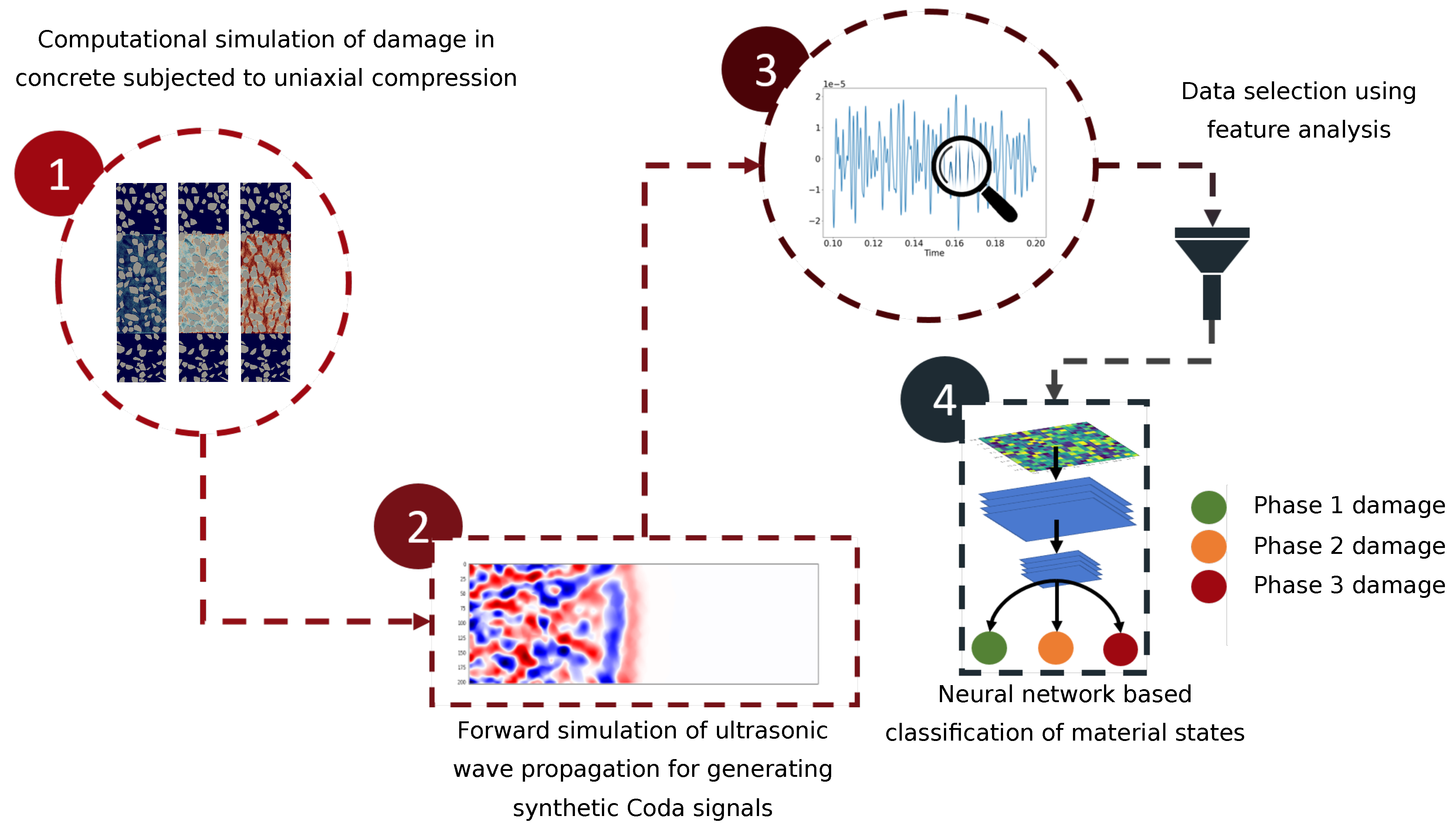
This section presents a brief summary of the entire workflow illustrated in
Figure 1. First a realistic synthetic concrete specimen was generated using the in-house Concrete Mesostructure Generator (CMG) code [
31]. Next, a uniaxial compression simulation was performed on the synthetic concrete specimen by means of the Discrete Element Method [
29]. The mesostructure snapshots containing information about the spatial distribution and evolution of microcracks are used as input for finite-difference simulations of wave propagation with multiple sources and receivers [
30]. The time series signals, obtained from the wave propagation simulations, which are the displacement components
x,
y and
z recorded at predefined receiver locations for over 40,000 time steps, are then reformatted (reshaping a vector into an array) as an image before being fed to a CNN classifier. To increase the accuracy of the classifier, the averaged envelope was used to reduce the dataset. The performance of the classifier was significantly improved when using the reduced dataset for training the CNN classifier. Note that in this paper, the word ‘coda wave’, ‘wave’, ‘signal’ and ‘datapoint’ refer to the same item and are used interchangeably.
The aim of using simulated data for damage classification is not only to overcome the labor intensive effort in generating real coda data in the laboratory but also to facilitate a real time ultrasonic-based damage assessment system of a concrete structure prior to the acquisition of the actual data, provided that important details of the simulated processes (damage evolution and ultrasonic wave propagation) are appropriately captured in the respective numerical simulations.
3. Simulation of Synthetic Concrete Mesostructures Subjected to Uniaxial Compressive Loads
In this section, synthetic concrete mesostructures subjected to various levels of compressive loads are generated. The morphology of plain concrete is characterized by a distribution of coarse and fine aggregates (up to a volume fraction of 60–70%) that are embedded in a cementitious matrix (host) material. When concrete specimens are subjected to external loads, these aggregates induce highly disordered and complex stress and displacement fields. Under increasing loads, microcracks first initiate in the vicinity of the aggregates. These microcracks later coalesce to form localized macrocracks [
32]. Hence, in order simulate damage processes, especially the pre-peak diffuse damage due microcracking, it is essential that the heterogeneity of concrete at the mesoscale and the distribution of the aggregates are taken into account. To this end, the open-source Concrete Mesostructure Generator (CMG, ([
33])) developed by the authors was used to generate an ultra-realistic concrete specimen in which the coarse aggregates are explicitly resolved. The physical dimensions of the synthetic concrete specimen is
cm. Voxel resolution of the specimen is
million voxels. Each voxel is of size
mm. The total volume fraction of coarse aggregates in this specimen is 31.11% with
mm and
mm.
To simulate the load induced morphological and material changes to the concrete specimens, we use the Discrete Element Method (DEM). DEM has demonstrated its capability in modeling materials with a certain degree of discontinuity in the internal structure such as concrete and therefore it is well-suited for modeling the damage process in concrete. The method is capable of simulating realistic crack patterns of concrete under mechanical loadings (see e.g., [
29,
34]). Nevertheless, the DEM simulation requires the calibration of the contact parameters prior to the analysis and is generally not easily accomplished directly from laboratory tests.
According to DEM, a granular material (such as concrete, rock) is described by a dense packing of discrete elements that are linked together by cohesive frictional forces. Within the medium, the induced forces are transmitted via a contact network between the discrete elements and the dynamics of these discrete elements is governed by Newton’s second law [
35]. The contact network is first established and updated by identifying the elements and their nearest neighbor interactions. The concrete constitutive model proposed in [
36] is adopted in this work. The interaction of the particles under tension in normal direction is governed by a linear damage softening law and the tangential behavior of contact is based on the modified Mohr-Coulomb frictional law. Details of contact description can be found in [
37].
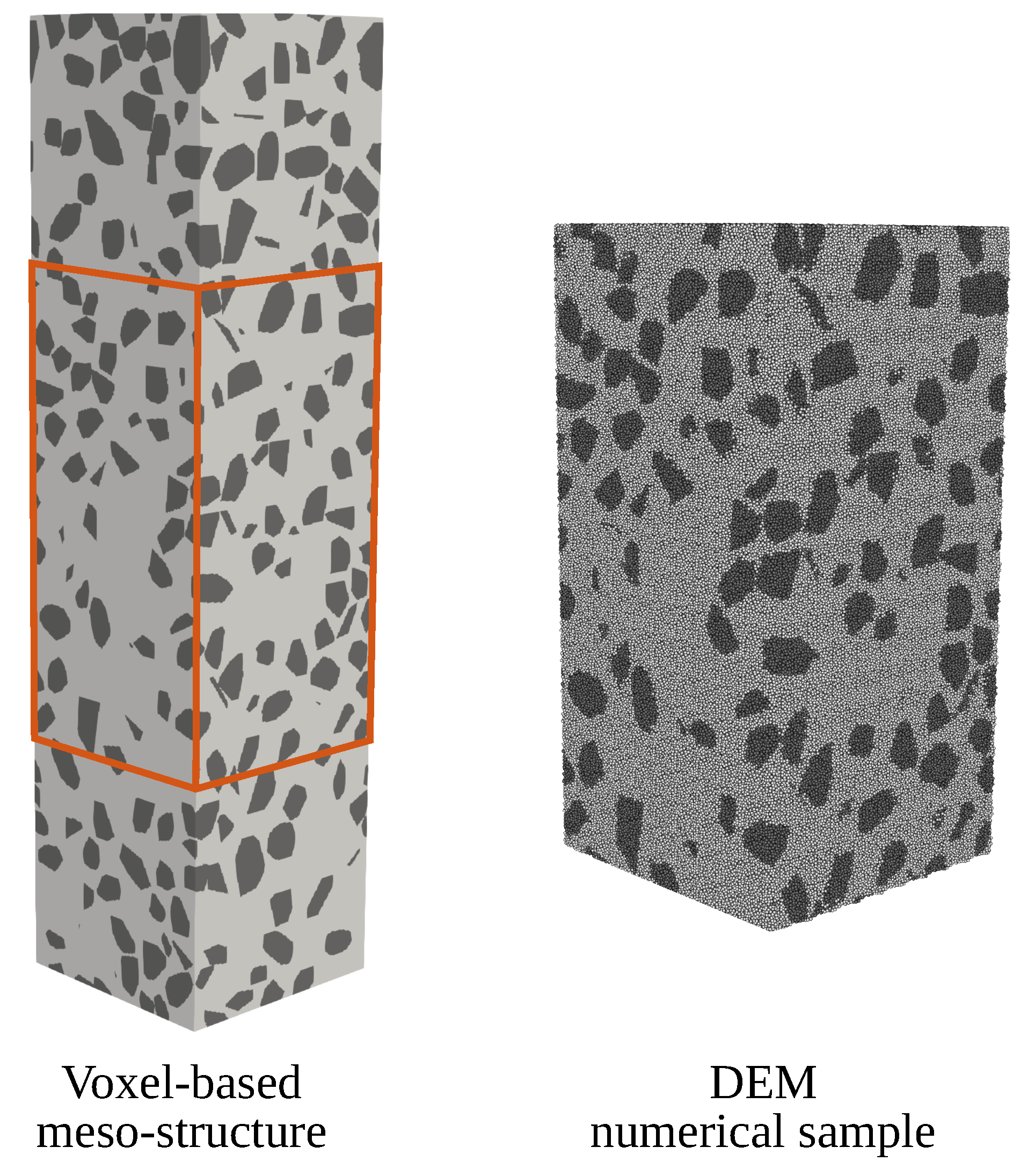
The DEM model is resolved using 2.4 million discrete elements with radius 0.5 mm. Next, the voxelized mesostructure was used to assign the material properties to all discrete elements. Here, only a region in the center of the voxelized mesostructure is considered (z = 10 to 30 cm) and denoted as “affected region”, as highlighted by the orange frame in
Figure 2. The contact parameters considered in the uniaxial compression simulation are listed in
Table 1.
The DEM uniaxial compression test is simulated as follows: The displacement control loading condition is simulated be prescribing a constant velocity of 10 mm/s on three layers at the top surface, while the position of particles at the bottom face is fixed. To simulate the frictionless loading system, transversal displacements at the top and bottom surfaces are set free. To ensure numerical stability and a fast convergence of the dynamic DEM model to a static response, a numerical damping it set to 0.2 and the average time increment is specified at 1.38 × 10
s. In this work, the DEM simulation was performed using an open-source DEM software ‘wooDEM’ [
38].
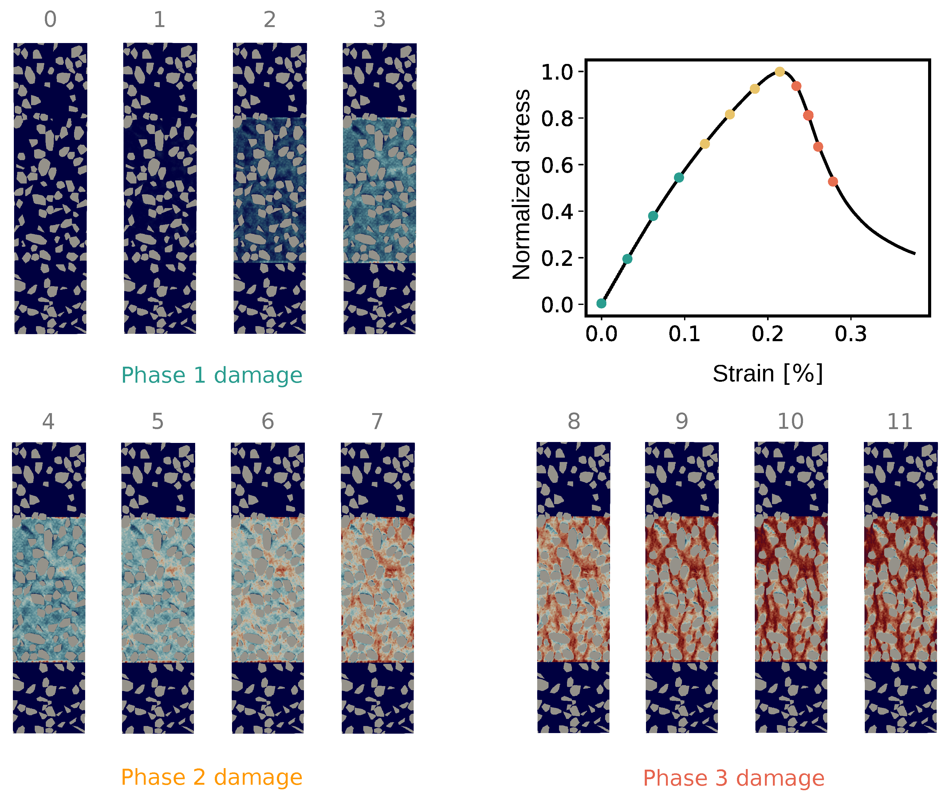
From the DEM simulation, a total of 12 mesostructure snapshots are selected and grouped into 3 labels (see
Figure 3) “Phase 1 damage” (green colored markers), “Phase 2 damage” (yellow-colored markers) and “Phase 3 damage” (red colored markers).
Figure 3 (top right) shows the normalized compressive stress
vs. the strain obtained from the DEM simulation. Let
denote the uniaxial compressive strength of the specimen. In the regime denoted as “Phase 1 damage” (
), microcracks start initiating in the specimen, however, the deformation predominantly is elastic at this early stage (see
Figure 3). The regime “Phase 2 damage” (
) is characterized by the growth of diffusely distributed microcracks, also known as “failure precursors”. “Phase 3 damage” is related to the post-peak regime associated with multiple macrocracks opening parallel to the loading direction due to the coalescence of the microcracks.
4. Synthetic Coda Wave Generation
Numerical wave propagation simulations are performed on each of the 12 mesostructures. A rotated staggered-grid (RSG) finite-difference scheme [
30] is used to propagate the seismic wavefield in the forward simulations. The RSG uses rotated finite-difference operators, leading to a distribution of modeling parameters in an elementary cell where all components of one physical property are located only at one single position. This can be advantageous for modeling wave propagation in anisotropic media or complex media, including high-contrast discontinuities, because no averaging of elastic moduli is needed [
39]. Concrete is a strongly heterogeneous and densely packed composite material. Due to the high density of scattering constituents and inclusions, ultrasonic wave propagation in this material consists of a complex mixture of multiple scattering, mode conversion and diffusive energy transport. With previous studies in 2D and 3D [
40,
41] it was shown that the RSG-technique is well-suited for such applications. A finite-difference operator of second order is used in time as well as in space. The surfaces of the concrete model are implemented as a free surface using two layers of vacuum. These vacuum layers mimic the impedance of the concrete specimen-atmosphere boundary. A typical simulation with a model size of
cm
consists of 32 million grid points (spatial increment
m). A simulation with
time steps takes about 3 hours on three nodes on a mid-size cluster computer.
Simulation Set up and Time Series Dataset Acquisition Procedure
For the mortar matrix we use a P-wave velocity of m/s, a S-wave velocity of 2250 m/s and a density of 2050 kg/m and for the aggregates a P-wave velocity of m/s, a S-wave velocity of 3330 m/s and a density of 2950 kg/m is assumed.
To mimic the attenuation characteristics typically observed in ultrasonic laboratory measurements of concrete specimens, a homogeneous intrinsic attenuation has been applied in the Finite-Difference scheme according to [
42], with the parameters
MPa,
MPa for the aggregates, and
MPa,
MPa for mortar matrix. Additionally, a frequency-dependent attenuation with a single Maxwell body with a minimal
at
kHz is simulated.
For the numerical samples experiencing material damage, the elastic wave velocities are reduced based on the damage parameter
d. For all simulations, a wavelet with a central frequency of
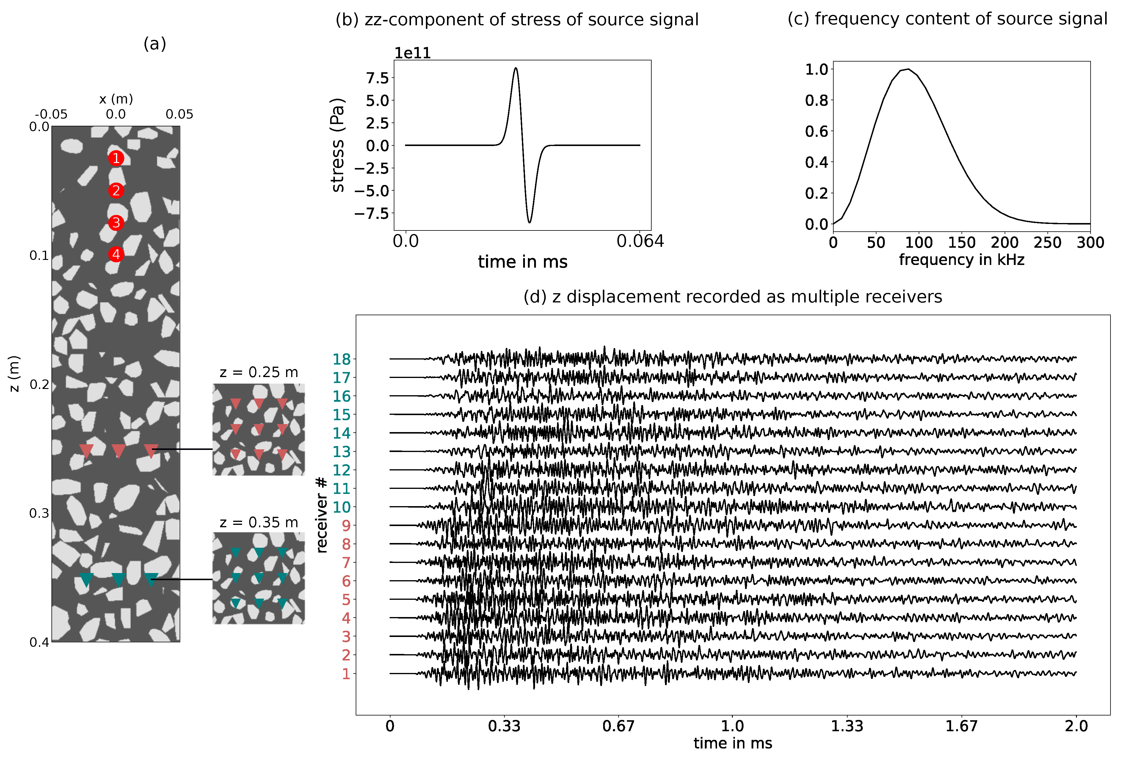
kHz is used, as this central frequency lies within the proposed frequency range for concrete with an ideal signal-to-noise ratio (ISO 1920-7:2004). Sources are implemented as body force sources, with components
and
being nonzero (
Figure 4b,c). The time increment is set to
s to ensure numerical stability. In all simulations, multiple sources and receivers were implemented as follows:. Four source locations were considered in the analysis at positions
cm, 5 cm,
cm and
cm.
Figure 4a shows the setup for the wave propagation simulation. The red circles denote point sources. At positions
and 35 cm, two sets of receivers (red and green triangles) are distributed evenly on a 3-by-3 grid on the
-plane with a spacing of 2.5 cm. The receivers are denoted with ID:identifiers from 1 to 18. The receivers 1 to 9 (ID = 1–9) lie inside the damaged zone and the receivers with ID = 10–18 lie outside of the damaged zone. The data recorded are the displacement components
for over 40,000 time steps (i.e., for a total duration of 2 ms).
Figure 4 shows an example of temporal displacements
z recorded at 18 locations (also known as time series) corresponding to the first mesostructure shown in
Figure 3. In summary, from a single source and 18 receivers, we obtain a total of 18
displacement components
damage cases
time series signals. Considering 4 source locations, a dataset of 2592 simulated time series signals is generated.
5. Damage Identification Using Supervised Machine Learning
Having generated the dataset containing 2592 labeled data points (coda signals), the objective now is to use supervised learning to identify the state of a concrete specimen given a coda signal.
The possible states of the concrete specimen correspond to three labels associated with each data point (coda signal) i.e., (1) Phase 1 damage, (2) Phase 2 damage, (3) Phase 3 damage. We use a feed forward Convolutional Neural Network (CNN)-based classifier. CNNs are a special type of Artificial Neural Networks (ANN) which are designed specifically to handle inputs with large dimensions. Traditionally, CNNs were designed to classify conventional visual images, in which the pixel data of an image is fed into the network in terms of an array. In our case, the time series data were reshaped into a 2D matrix by first slicing the series data into multiple parts and then arranging these parts into an array consecutively one row after another. Details of data processing, CNN architecture as well as the results are presented in the forthcoming subsections.
5.1. Data Processing
A single complete time series signal in our case consists of 40,000 displacement values (corresponding to 40,000 time steps). Reshaping this one-dimensional array into a two-dimensional array produces an array of size .
To take into account the influence of signals at the initial state (corresponding to snapshot id 0), all signals of the respective source location are scaled by dividing the time series to the maximum amplitude of the reference signal. Thus, the reference time series signals (displacement components x, y, z at the zero-stress state) have the maximum values between and , and signals at the remaining steps are scaled appropriately.Thereafter, the dataset (2592 signals) was randomly shuffled, and 3/4 (1944 signals) of the shuffled dataset was used for training and 1/4 (648 signals) of the dataset was used for validation. The output is in the form of a one-hot encoding vector corresponding to each damage phase (i.e., the first label is [1,0,0], the next one is [0,1,0] and the final one is [0,0,1]).
5.2. CNN Damage Classifier
The CNN classified was constructed by tuning the hyperparameters in the architecture, such as convolutional and dense layers, number of filters, filter size, stride and the units of the dense layers. Such procedure was performed based on trial and error and the architecture was determined based on the accuracy metric. Other possible techniques for optimizing the hyperparameters can be found for e.g., in [
43,
44].
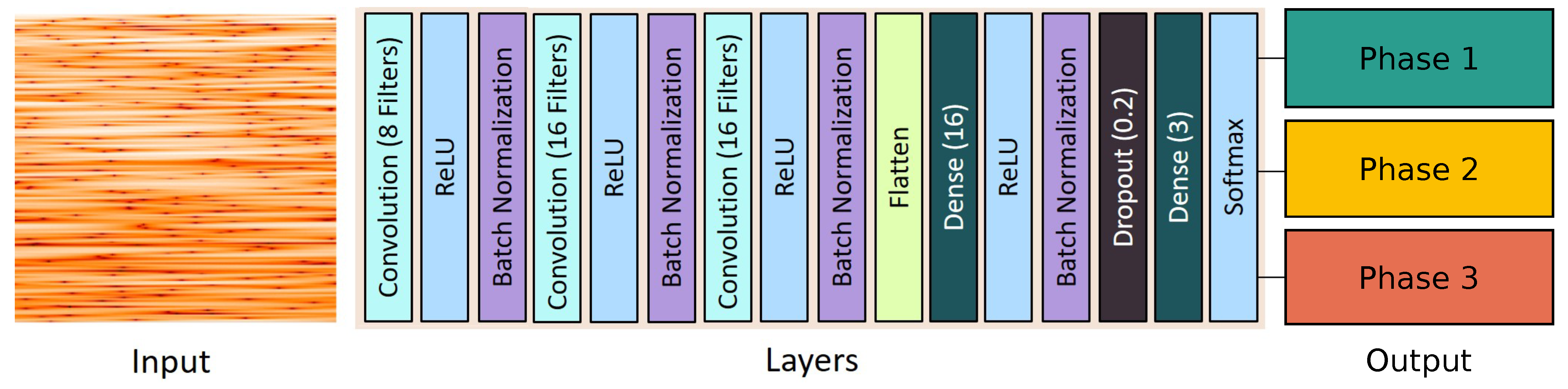
Details of the CNN architecture are presented in
Figure 5 and
Table 3. The NADAM algorithm [
45] was used as the optimizer and ReLU [
46] was used as the activation function across the network. This optimizer and the activation function was chosen because it provided the fastest convergence with highest accuracy among all optimizers available in the Keras library for this dataset. Furthermore, from the parametric study, it was found that at least 3 convolutional layers are required to achieve an adequate accuracy of the classifier. The loss function for back propagation is based on Categorical Cross Entropy function. The learning rate was set as 0.001 and the network was trained for 200 epochs with a batch size of 32.
5.3. Results
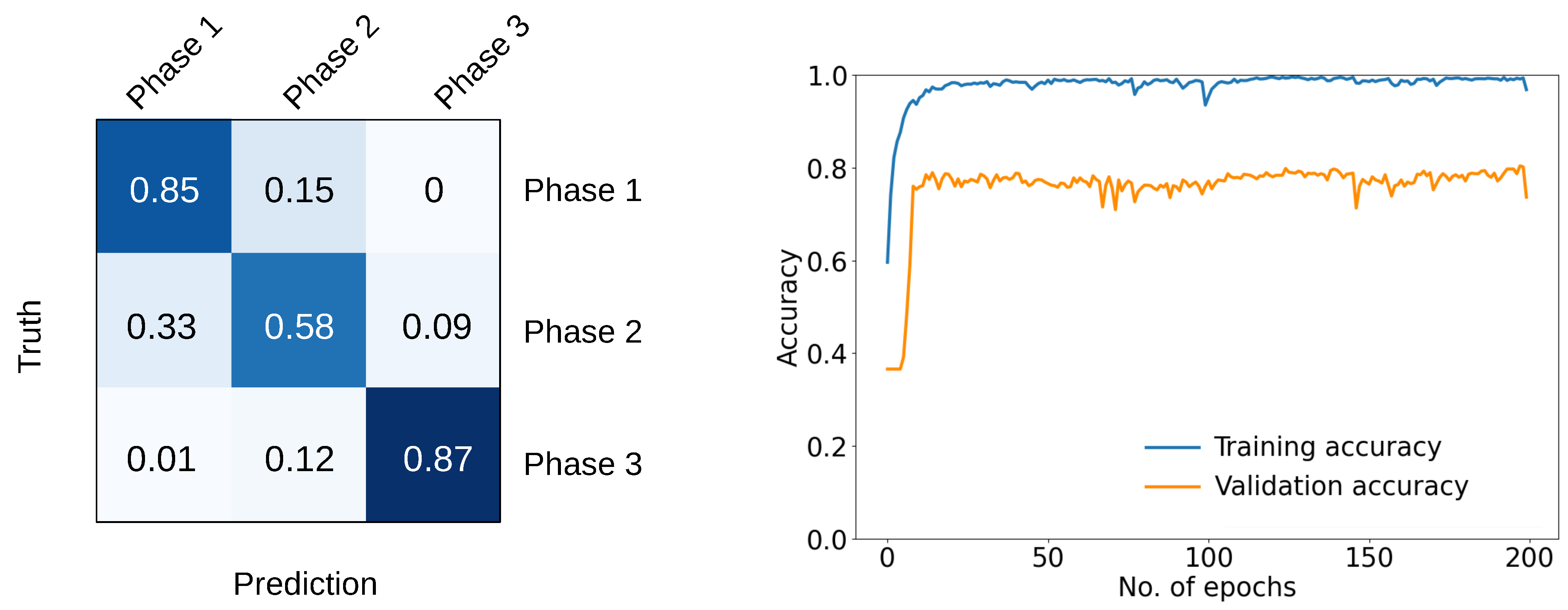
Figure 6 shows the training and validation accuracy. The validation accuracy is around 77%. The confusion matrix of the trained classifier is shown in
Figure 6.
The performance of the classifier using this architecture and the dataset is as follows:
Phase 1 damage: 85% of the signals corresponding to this phase were correctly identified. A total of 15% of the signals were wrongly identified as belonging to Phase 2 damage.
Phase 2 damage: Only 58% of the signals corresponding to Phase 2 damage i.e., pre-peak microcracking were correctly identified. Indeed 33% of the signals belonging to the class of Phase 2 damage were incorrectly classified as Phase 1 and 9% were incorrectly identified as Phase 3.
Phase 3 damage: 87% of the signals corresponding to this state were correctly identified. A total of 12% were misclassified as Phase 2 and 1% was wrongly classified as Phase 1.
6. Improvement of Accuracy Using Data Refinement
To improve the classification accuracy especially with regards to the correct identification of damage Phase 2, i.e., pre-peak microcracking of concrete, we analyze in this section an additional feature corresponding to the averaged envelope of the coda signal. Using this additional feature we generate a refined dataset. The averaged envelope of all the coda signals from the dataset (2592 signals) was computed by first finding the peaks in the signal over the complete signals and averaging these values. These averaged values were first segregated into different groups corresponding to each source location. These values were then normalized between 0 and 1 corresponding to each source location (the highest value in the group being set to 1 and lowest value as 0 and all the values in between scaled appropriately) before being plotted as a scatter plot.
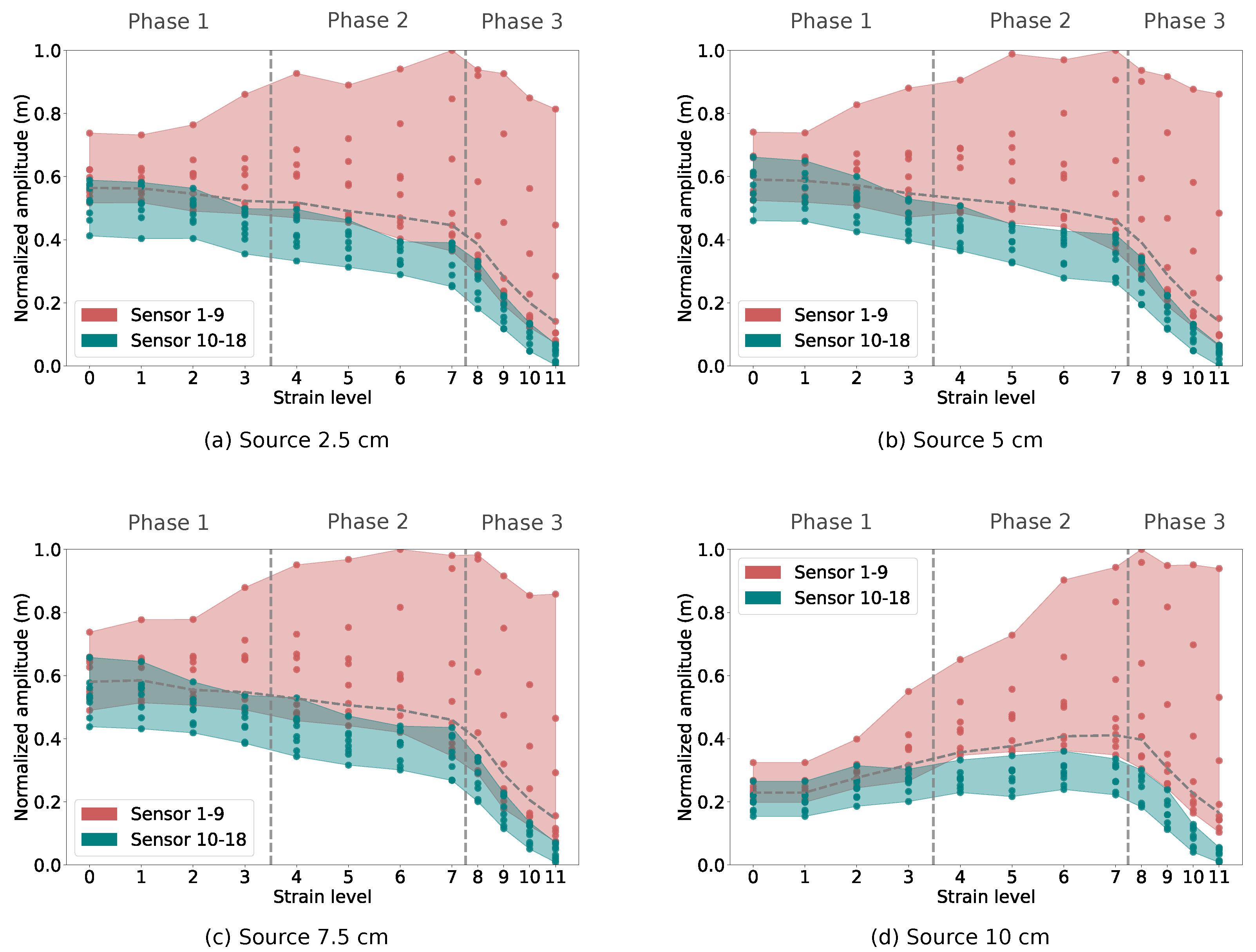
Figure 7 shows 4 different scatter plots of the normalized amplitude across the three damage phases. Each plot corresponds to a particular source location. The data in each plot is segregated according to the location of the receivers. A red background is applied to all data recorded by the receivers 1–9 (lie inside the damaged zone) and a green background is applied to all data recorded by the receivers 10–18 (see
Figure 5 for the receiver positions). The average value of this feature for a particular source is plotted as a function of increasing strain levels as a dashed line (horizontal) in
Figure 7. Furthermore, two vertical dash lines are placed in the plot to separate the three phases of damage. Two main conclusions can be drawn from the plot. First, this feature corresponding to the receivers inside the damaged zone (receivers 1–9) shows a high variance in comparison to the receivers present outside the damaged zone (receivers 10–18) for all source locations. Secondly, the excitation source (source at 10 cm, bottom right of
Figure 7), located inside the damaged zone, shows a unique pattern as compared to the other three cases, when the source was located outside the damaged zone. These observations are explained in more detail in the following section.
When the excitation point was located at 2.5 cm (
Figure 7, top-left) from the origin along the Z axis, the average of the features for this particular source location reduced with increasing damage. A similar trend is seen for the sources located at 5 cm and 7.5 cm, respectively. This trend can be explained as follows: when the strain level increases, the number of small microcracks present in the structure also increases. A higher number of microcracks present in the path of the source and receiver will reduce the energy present in the wave reaching the sensor because some part of the wave will be reflected back and only a portion will proceed forward at each microcrack. Thus, there is a general decrement in the average envelope value of the Coda signals with increasing strain level.
However, the trend observed for source location 10 cm (
Figure 7, bottom-right), which is located inside the damaged zone, is quite different. Here, the line of the average amplitude increases till the peak stress (end of Phase 2) and then decreases afterwards in the post-peak regime. Obviously, the presence of the source location inside the damaged zone affects the trend of the average line. In particular, in the plot from source 10 cm, we observed that the overall increase of the average amplitude from the red area before the crack localization Phase is more pronounced. Interestingly, the averaged amplitude of signals from the green area also increases slightly prior to the crack localization. This might be related to the crack orientation parallel to the sender-receiver orientation, which guides the waves toward the receivers. As long as the damage level is weak, this effect seems to overcompensate the effect of stiffness reduction which is the dominant effect in the other three plots. As soon as crack localization starts (Phase 3), the strong stiffness degradation finally governs the decrease of the amplitudes. From our interpretation, this could be a feature, in addition to differentiating diffuse microcracking and localized fracture, could provide information of the damage anisotropy (microcrack orientation). Nevertheless, the potential use of this observation for damage identification still must be validated according to the analysis of measured coda signals in the laboratory. This will be performed in the future.
When comparing the effect of receiver location, it can be observed in each graph in (
Figure 7) that the variance is evidently higher for the group of receivers present inside the damaged zone. It is quite clear that the location of the receivers has a significant effect on the recorded displacement data. The envelope plots provide a simple method to differentiate between “good” and “bad” data. Good data refers to data with a small variance relative to the average line, while bad data refers to data with a large variance. Therefore, we have filtered out the data corresponding to the receiver locations 1 to 9 and the source 10 cm located inside the damaged zone. Thus, the training dataset reduces to 972 time series signals.
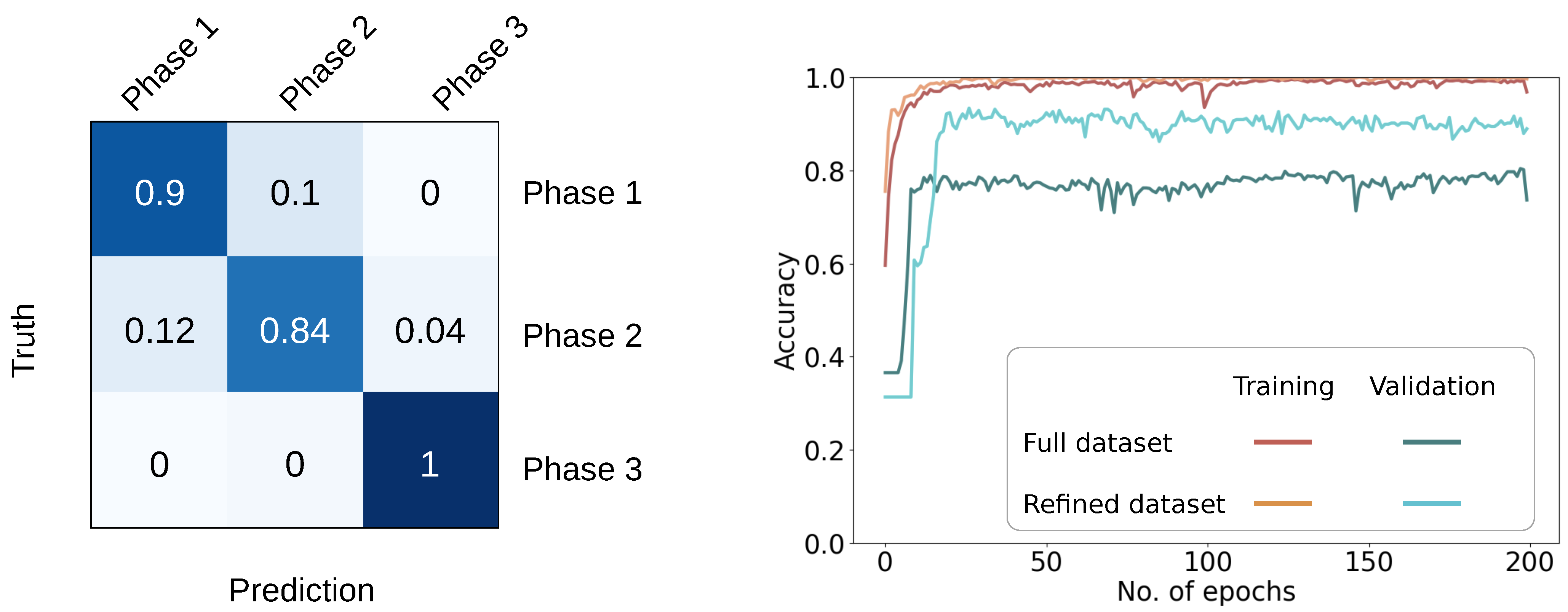
Figure 8 left shows the confusion matrix and
Figure 8 right shows the accuracy of the training and validation obtained from the full and the reduced dataset, using the same CNN architecture. We observed that the accuracy of the validation with the reduced dataset is approximately 90%, which is a significant improvement as compared to taking the full data set, where an accuracy of approximately 77 % was obtained and unsatisfactory prediction of Phase 2 damage (58% accuracy).
Furthermore, it is worth pointing out that the misclassification is mostly on the prediction of Phases 1 and 2. This is attributed to the gradual transition between the two Phases. As can be seen in
Figure 3, damage evolution at load levels 3 and 4 share high similarity in the spatial distribution of damage, characterized by the overall degradation of mortar matrix in the pre-peak regime. Such results imply the challenge of correlating thoroughly the coda signal with the corresponding damage Phase, especially when applying the method on measured data.
Lastly, the performance of the classifier can also be evaluated by other metrics, namely the Precision, Recall and F1 score. The metric evaluation for each class is shown in
Table 4. From the analysis, the performance of the classifier is good.
7. Conclusions
A computational methodology for detection of damage in concrete under compression loading using synthetic Coda waves has been proposed in this paper. The microcrack growth evolving in realistic virtual concrete specimen, characterized by a realistic aggregate size distribution was simulated using the discrete element method (DEM). The damage evolution in the pre-peak regime as well as the formation of localized macrocracks in the post-peak regime have been recorded as different stages and used for computational wave propagation simulations. The simulated ultrasonic signals were used to train a convolutional neural network (CNN) to predict the corresponding damage class (Phase 1: Elastic deformation and microcrack initiation, Phase 2: Pre-peak microcracking and Phase 3: Microcrack coalescence and post-peak crack localization). It was observed that the performance of the CNN using the full dataset was unsatisfactory. Therefore, a feature based on the envelope of the coda signals was used to refine the dataset. The trendline of the average envelope plotted over the strain level shows a remarkable difference when evaluated for the sender located inside the damaged zone as compared to the source located outside of the damaged zone of the virtual specimen. This feature can potentially be used to derive information on the microcrack orientation. It was also observed that a much larger scatter of the average of the envelopes of the Coda signals was obtained for receivers located inside the damaged area as compared to the receivers located outside of this zone. When filtering the signals from receivers located inside the damaged zone, i.e., using a reduced data set, the accuracy of the CNN with the same architecture was considerably improved.
Based on the results, the following conclusions can be drawn:
The application of ultrasonic measurement in damage assessment of concrete structures is an active and yet challenging research field. The underlying challenge arises from complicated damage process in concrete and the high sensitivity of the coda wave especially to the environmental factors, which do not contribute to damage. Thus, computational approaches can assist experimental work in understanding the effect of damage processes on the characteristics of coda signals, while excluding the effect of the environmental factors.
With a suitable feature analysis method, CNN can be used as a supplementary tool for ultrasonic-based damage identification in concrete.
It has been demonstrated that data obtained from a damaged region has a negative effect on the performance of the CNN classifier. In practice, the damage location is generally not known a priori, thus, a filtering tool should be thoroughly formulated to enhance the robustness of the CNN classifier.


 ,
, 


