
Theoretical Study of Some Angle Parameter Trigonometric Copulas

Department of Mathematics, University of Caen-Normandie, 14032 Caen, France
Modelling 2022, 3(1), 140-163; https://doi.org/10.3390/modelling3010010
Submission received: 8 February 2022
/
Revised: 5 March 2022
/
Accepted: 7 March 2022
/
Published: 10 March 2022
Abstract
:Copulas are important probabilistic tools to model and interpret the correlations of measures involved in real or experimental phenomena. The versatility of these phenomena implies the need for diverse copulas. In this article, we describe and investigate theoretically new two-dimensional copulas based on trigonometric functions modulated by a tuning angle parameter. The independence copula is, thus, extended in an original manner. Conceptually, the proposed trigonometric copulas are ideal for modeling correlations into periodic, circular, or seasonal phenomena. We examine their qualities, such as various symmetry properties, quadrant dependence properties, possible Archimedean nature, copula ordering, tail dependences, diverse correlations (medial, Spearman, and Kendall), and two-dimensional distribution generation. The proposed copulas are fleshed out in terms of data generation and inference. The theoretical findings are supplemented by some graphical and numerical work. The main results are proved using two-dimensional inequality techniques that can be used for other copula purposes.
Keywords:
copula; two-dimensional modeling; trigonometric function; multivariate distributions; dependencePACS:
62H991. Introduction
Multidimensional functions called copulas are important in modeling multivariate random variables and understanding their dependence structures. They find their origin and prime property in the Sklar theorem (see [1]). Mathematically, for any integer n, a n-dimensional copula can be defined as a cumulative distribution function defined on with standard uniform marginal distributions. For the purposes of this article, the definition of a two-dimensional copula in the absolutely continuous case is given below.
Definition 1.
In the absolutely two-dimensional continuous case, the functionis a two-dimensional copula if and only if
- for any;
- andfor any;
- the two-increasing property holds:for any.
This definition has a certain flexibility, but the main critical point remains the validity of the two-increasing property. On the practical side, copulas are crucial for estimating and interpreting the correlations of measures involved in real or experimental phenomena. Due to the plurality of possible phenomena of interest, a large number of copulas with various attributes are necessary. This has motivated researchers over the years to introduce valuable copulas, and apply them in concrete, real-life scenarios. The Frank, Gumbel–Hougaard, Ali–Mikhail–Haq, Joe, Farlie–Gumbel–Morgenstern, Clayton, Plackett, Raftery, elliptical, Fréchet, Galambos, and Marshall–Olkin are some of the classical copulas. Their definitions are based on motivated transformations of power-polynomial–exponential–logarithmic functions. They have specific qualities that make them of great interest in the context of random dependence modeling. Further details on these copulas can be found in the books of [1,2,3,4].
Recently, a lot of attention has been paid to copulas defined (partially or not) with trigonometric functions. The inclusion of trigonometric functions in this context confers on the copula some oscillating features that are appropriate to model the correlations into phenomena of periodic, circular, or seasonal nature. In particular, they are ideal for analyzing correlations involved in movement data, circular data, and environmental data. The theory of the classical trigonometric copulas can be found in [5,6,7,8,9,10,11]. For practice, we refer to [12,13,14,15,16]. Furthermore, the R package named Cylcop, recently developed by [17], gives the trigonometric (and circular) copulas a new dimension of applicability.
In this article, we present and study trigonometric copulas depending on a tuning angle parameter. They are derived from the very general family of copulas (not especially trigonometric) introduced in [18], but with the importance of the angle parameter in mind. To be more specific, the proposed copulas are defined by the following form:
where is a simple one-dimensional function involving a trigonometric function, and is the angle parameter that only modulates this trigonometric function. Despite the potential for modeling correlations into periodic, circular, or seasonal phenomena, this area of research appears to have received little attention; none of the references [5,6,7,8,9,10,11] consider such an angle parameter approach. Thus, we describe the most intuitive of such angle parameter copulas, and study them on the theoretical side with a maximum of details. In particular, we emphasize the optimal set of values for such that the corresponding copula remains valid. We determine the expressions of the corresponding copula density, survival copula, and survival copula density. Some mixed trigonometric copulas are also given. Then, we examine a maximum of theoretical properties of the proposed angle parameter copulas, including symmetry properties, quadrant dependence properties, copula ordering, various expansions, tail dependences, medial correlation, Spearman correlation, Kendall correlation, and two-dimensional distribution generation. Data generation and inference from the proposed copulas are sketched. The theory is illustrated by means of graphics. The proofs of the main results are based on some two-dimensional inequality techniques that can be of independent interest.
2. Cosine Angle Parameter Copula
This section is devoted to a simple cosine copula with an angle parameter.
2.1. Definition and Graphics
The following proposition presents the considered cosine copula.
Proposition 1.
The functiondefined by
withis a valid copula.
Proof.
Let us prove the main points defining an absolutely continuous two-dimensional copula, as recalled in Definition 1.
- For any , we have , and, for any , .
- For any , we have and, similarly, for any , .
- For any , using standard derivation techniques, simplifications and factorizations, we have
Let us prove the two-increasing property: .
Since , we have . It follows from the inequality , applied with that
where
and
Let us prove that and .
For , we can remark that . So as a product of positive terms.
For , it follows from the inequality , applied with that
where
We have
implying that is a decreasing function with respect to . Therefore, for any , we have
with
Let us prove that for any . First, is a continuous function for , and is a compact set, so the maximum and minimum of on this set are attained. Let us now perform a critical points analysis. We have
Therefore, we have and if and only if
- and ; or
- and which implies that , so this case is excluded; or
- and which implies that , so this case is excluded; or
- and , which implies that and , which is a polynomial of degree 2 with the discriminant equal to . Therefore, there is no (real) solution.
As a result, there is only one critical point for , and it is . This point clearly gives a maximum value for since . Since there is no other critical point, has a “two-dimensional decreasing pattern”, and the minimum value of is attained on point(s) on the borders of . Therefore, for any , we have
As a result, is a valid two-dimensional copula. This ends the proof of Proposition 1. □
Remark 1.
For the more restrictive case, we can prove the two-increasing property in a more simple and direct manner. We have
Since , we have , and by applying the inequality for any with , we get
Since , we have and . Thus
The two-increasing property is proved. This ends this alternative proof for .
For the purposes of this study, we call the copula in Equation (1) as the cos-copula. It has the feature of having a tuning angle parameter that modulates its correlation features. For , we clearly have ; the cos-copula is reduced to the independence copula. Furthermore, we can remark that the cos-copula is still valid for because of the evenness of the cosine function. We can, thus, define the cos-copula with without loss of generality.
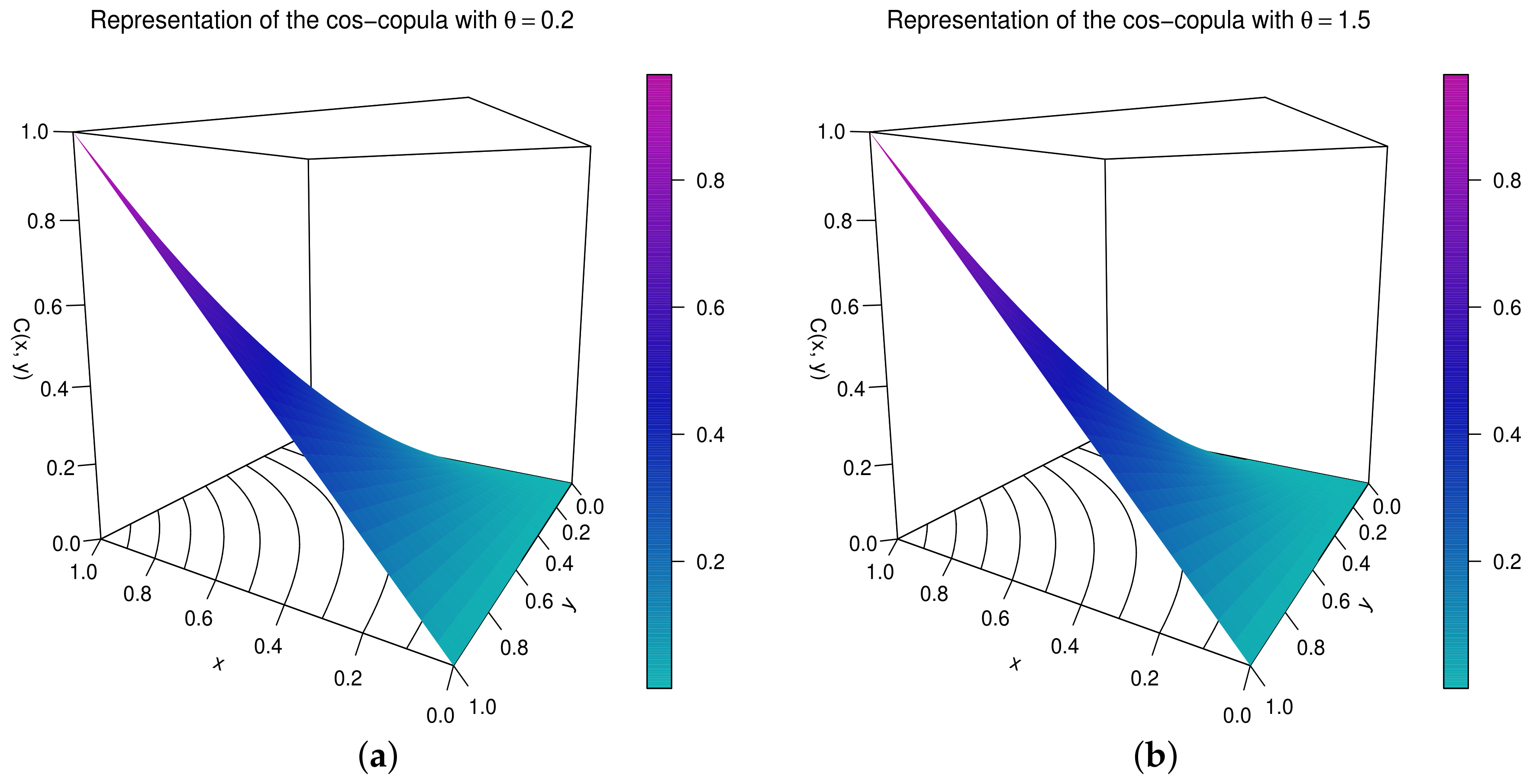
To end the presentation, Figure 1 represents the two-dimensional plot of the cos-copula for selected values of .
From Figure 1, we see that the parameter skews the triangular shape of the cos-copula.
The next parts are devoted to the functions related to the cos-copula, as well as its main properties.
2.2. Related Functions
The density associated with the cos-copula is the function given by
It is worth noting that which can be negative for some values of . In particular, is not a copula for . In this sense, if we restrict our attention to the interval , is the optimal set of values for .
As usual, the copula density can be involved in various moment-type measures, and estimation methods (see, for instance, Refs. [13,17]).
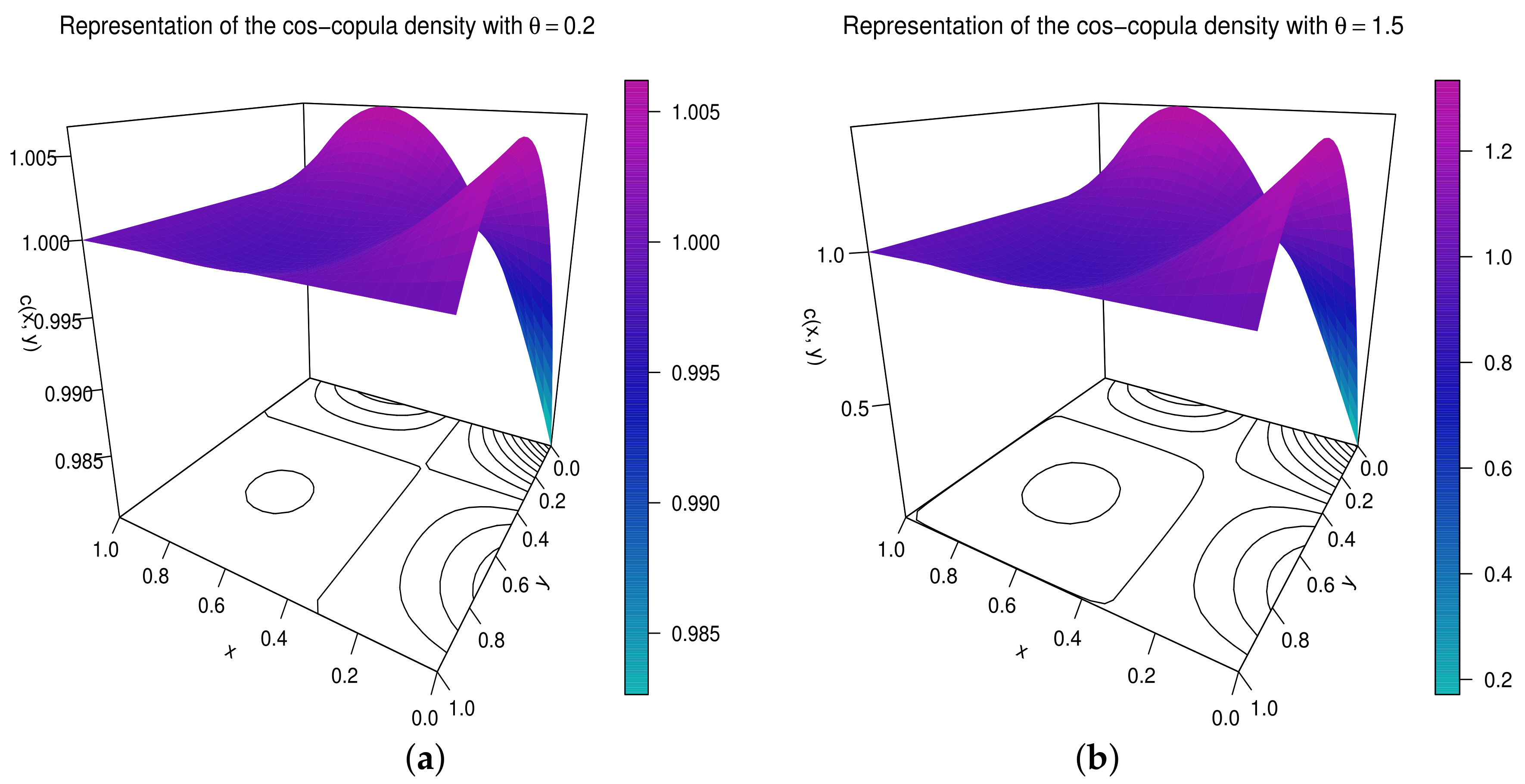
Figure 2 represents the two-dimensional plot of the cos-copula density for selected values of .
Thus, we see how the parameter affects the overall shape of the cos-copula density.
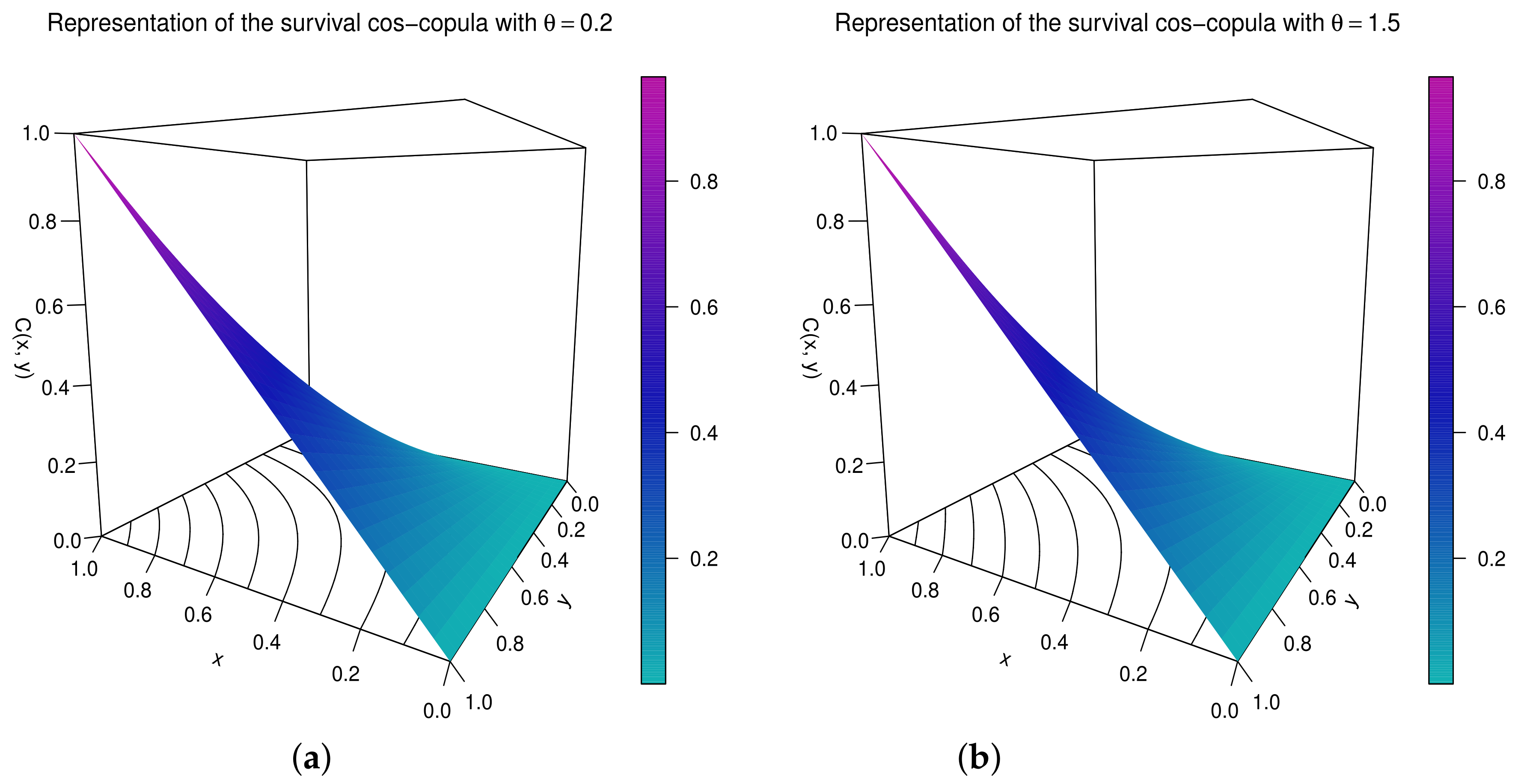
As a last important function, the survival cos-copula is the function defined by
It defines a valid copula, which is also a new trigonometric copula with an angle parameter represented by .
Figure 3 represents the two-dimensional plot of the survival cos-copula for selected values of .
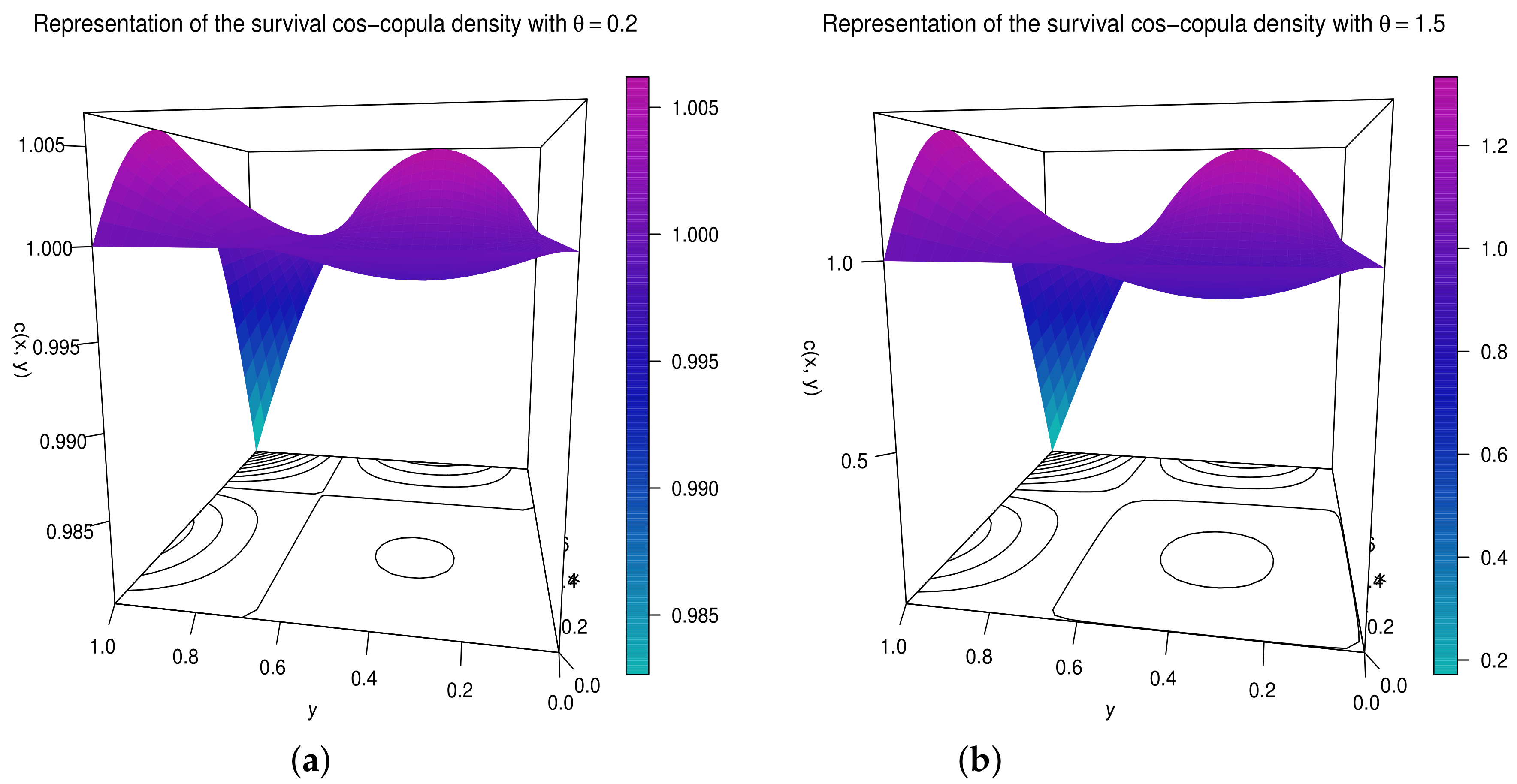
The density associated with the survival cos-copula is given by
To have an idea of its shapes, Figure 4 shows the two-dimensional plot of the survival cos-copula density for selected values of .
Because any convex linear combination of copulas is a copula (see [1]), the cos-copula can be used in a variety of new mixed copulas. For instance, we can consider the following mixed cos-copulas:
- Mixed copula 1: For any angle parameters and and , by setting , a possible mixed copula is given as
- Mixed copula 2: A second example is
They are also new angle parameter trigonometric copulas by construction.
2.3. Properties
We now list the important properties of the cos-copula as specified in Equation (1).
- As already mentioned before:
- –
- For , it is clear that . Therefore, the cos-copula is reduced to the independence copula.
- –
- If we restrict our attention to the interval , the set is the optimal set of values for for validating as a copula.
- For any , we have . Hence, the cos-copula satisfies the negative quadrant dependence property (see [21]).
- The cos-copula is symmetric since for any .
- The cos-copula can be expressed under various analytical forms. Two of them are given below:
- –
- In terms of simple cosine-sine functions, we can writeWe thus see the intrinsic analytical complexity into the cos-copula.
- –
- In terms of power series, by using the cosine series expansion and binomial formula, we getIn particular, upon differentiation with respect to x and y on the interior of the domain of convergence, one hasThis expansion can be used in a variety of mathematical applications, such as determining various moment-type measurements.
- By arbitrary taking , we notice thatAs a result, the cos-copula is not Archimedean (see [1]). In other words, there is no generator function such that , where denotes the pseudo-inverse of .
- The cos-copula is not radially symmetric since there clearly exists such that .
- As any copula, the Fréchet–Hoeffding bounds can be expressed as follows: For any , we have .
- Thanks to the Kober inequality, the following inequality holds:where with refers to the Farlie–Gumbel–Morgenstern (FGM) copula (see [1]). Since , the cos-copula and FGM copula are involved in a complete copula ordering.
- For any , the two following results are obtained:andHence, the cos-copula has no tail dependence (see [1]).
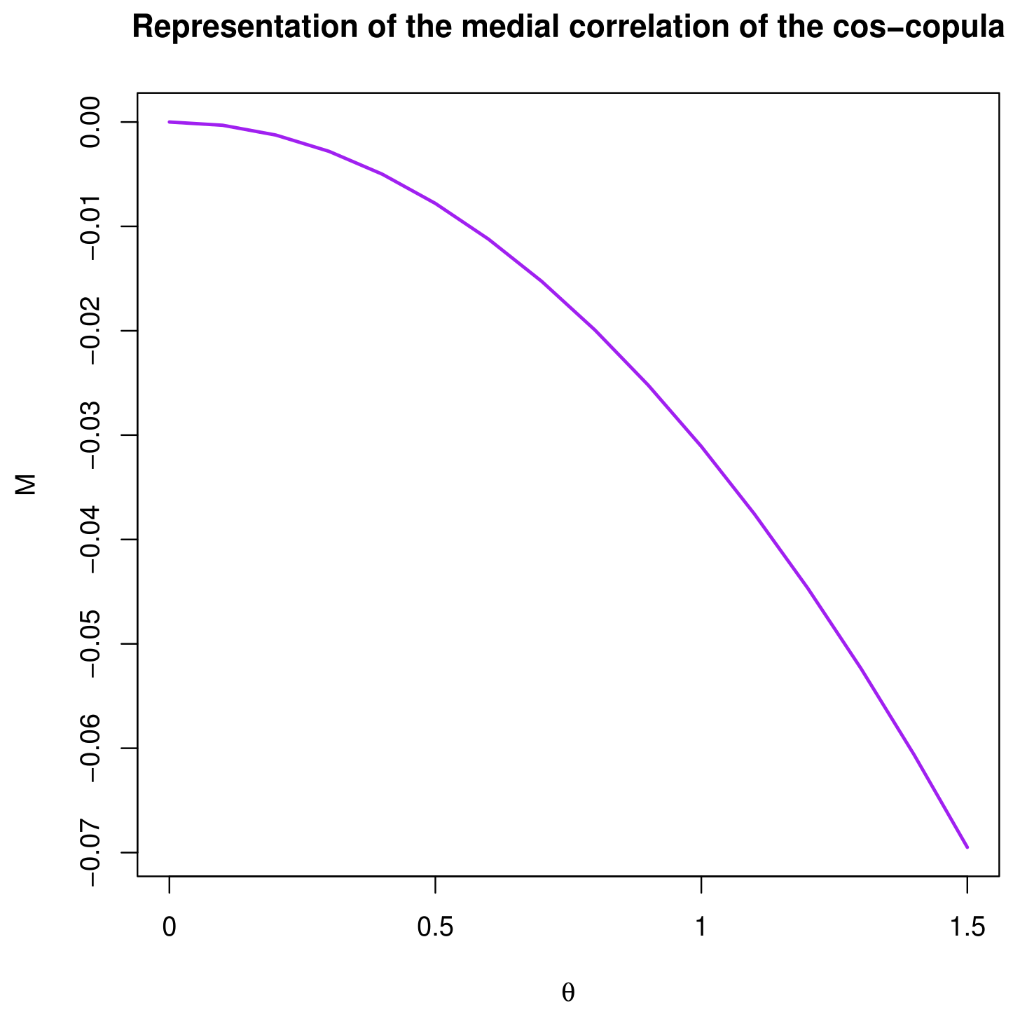
- The medial correlation of the cos-copula is defined byIt is clearly a decreasing and negative function with respect to for , with for and for . Figure 5 represents the medial correlation for .Thus, the cos-copula has a weak medial correlation with .
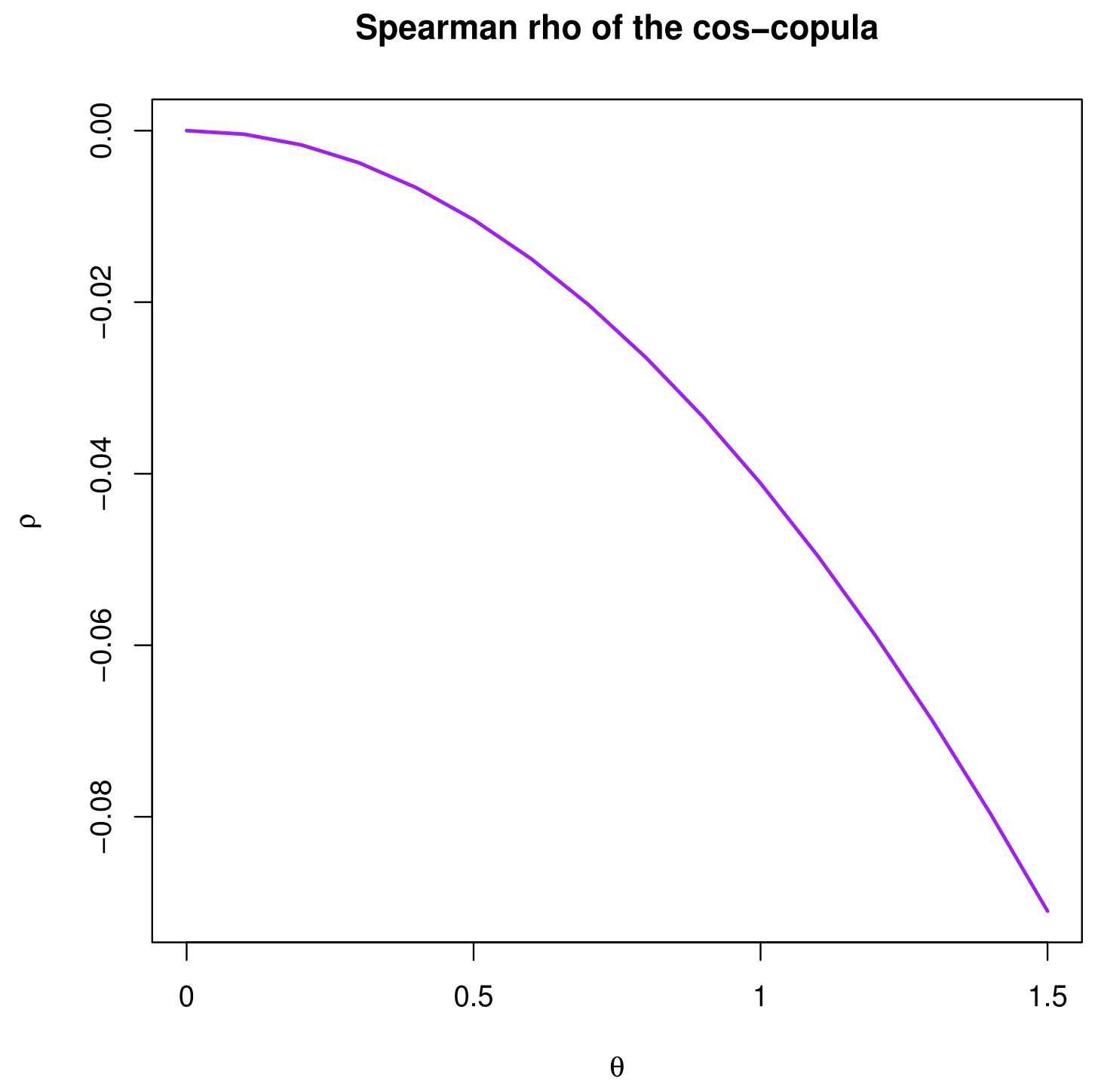
- A useful dependence measure based on copula is the Spearman rho (see [1]). The Spearman rho of the cos-copula, as an example of copula, is defined by
Based on well-known mathematical techniques, the following proposition provides a mathematical expression for this measure.
Proposition 2.
The Spearman rho of the cos-copula can be expressed as
where denotes the cosine integral defined by , denotes the sine integral referred by , and is the Euler–Mascheroni constant.
Proof.
The desired result follows immediately.
The proof of Proposition 2 ends. □
Thus, is a decreasing function with respect to for , with for and for . Figure 6 represents the Spearman rho for .
In light of the above results, the cos-copula is adapted to model weak negative correlations.
Remark 2.
Based on Equations (6) and (8), upon integration over and some arrangements, the following series formula holds:
Of course, this result is of independent interest to our copula study. It is, however, fascinating to see the versatility in the nature of the functions involved, i.e., logarithmic, special integral function, cosine function, and Euler–Mascheroni constant.
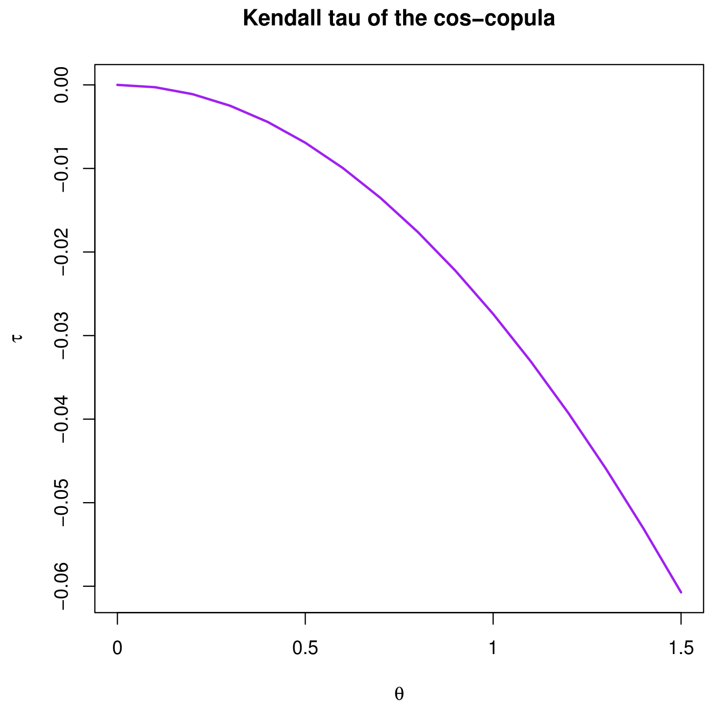
- In complement of the Spearman rho, we can present the Kendall tau of the cos-copula. It is defined by
The closed form expression for is unmanageable due to the complexity of the product function . We can, however, state that it is a decreasing function with respect to for , with for and for . Figure 7 represents the Kendall tau for .
The small values of confirm the fact that the cos-copula is ideal to model weak negative correlations.
- The cos-copula opens some interesting perspectives in distribution theory and modeling. The most immediate of these perspectives is the creation of simple and new two-dimensional distributions with cumulative distribution functions of the following form: , sowhere and denote two cumulative distribution functions. This gives two-dimensional trigonometric distributions, which seem slightly underexplored in the literature. By considering the exponential distribution as the parent, we may define the cos-two-exponential distribution by the following cumulative distribution:and for . To understand the importance of the trigonometric distributions in theory and practice for the uni-dimensional case, we may refer to [22,23].
2.4. Data Generation and Inference
The most straightforward method of generating random data (or values) from a distribution defined by a copula is what might be termed the inverse conditional method. For any positive integer n, with the aim of generating n data from the cos-copula, this method may be described as follows:
- Generate n data from a random vector , where S and T are independent random variables with the uniform distribution over .
- Choose a value of .
- Consider the following “conditional function”:
- For any , compute such that .
- Then are n data generated from the cos-copula defined with the chosen .
Other methods exist (see [24]). Such simulated data can be used for computational tests, or estimation purposes.
On the other hand, in a data analysis scenario, the angle parameter is generally unknown. Its evaluation is, thus, of interest for precise data fitting, or at least to know if is close to 0 corresponding to the independent case, or close to , corresponding to the most highly correlated case. For this evaluation, it can be estimated from n data , that are susceptible to coming from the cos-copula distribution, by the maximum likelihood method; is thus estimated by
provided that it is unique. This estimation method ensures satisfying qualities to , such as underlying consistency and asymptotic normality, which are the basis for the construction of confidence intervals and statistical tests (see, for instance, Refs. [13,17]). At this point, concrete applications of the aforementioned techniques to real-world datasets remain a possibility.
3. Sine Angle Parameter Copula
This section completes the findings of the previous section; it is devoted to a simple sine copula with an angle parameter. This copula can be viewed as a parametric generalization of one copula introduced in [18]. Indeed, in ([18], Example 9), it is proved that the function defined by
is a valid copula. Among the questions that arise are:
- Can we replace the angle-value with a tuning parameter and, if so, what is its “optimal values set”?
- What are the related functions of such a copula?
- What are its theoretical properties?
The answers to these questions are given below.
3.1. Definition and Graphics
The following proposition presents the considered angle parameter sine copula.
Proposition 3.
The function defined by
with is a valid copula.
Proof.
Let us prove the main points defining an absolutely continuous two-dimensional copula, as recalled in Definition 1.
- For any , we have , and, for any , .
- For any , we have , similarly, for any , .
- For any , using standard derivation techniques, we haveLet us now study the sign of the above function by distinguishing the case and the case .Case : We can writewhereandLet us prove that and .For , let us first remark thatTherefore, since and for any , we haveFor , since , we have , implying that , and . It follows that . HenceThe two-increasing property is proved.
Case : For this case, we develop a strategy different to the previous case. We can write
where
and
Let us prove that and .
For , since , we have , which implies that .
For , since , the following inequality holds: for any , which implies that for any . It follows from this inequality applied with , the inequality
and the inequality: for any , applied with , that
Hence
The two-increasing property is proved.
As a result, is a valid two-dimensional copula. This ends the proof of Proposition 3.
□
For the purposes of this paper, we call the copula in Equation (9) as the sin-copula. Like the cos-copula, it has the feature to have a tuning angle parameter . Clearly, for , we have ; the sin-copula is reduced to the independence copula, and for , it is reduced to the copula in ([18], Example 9).
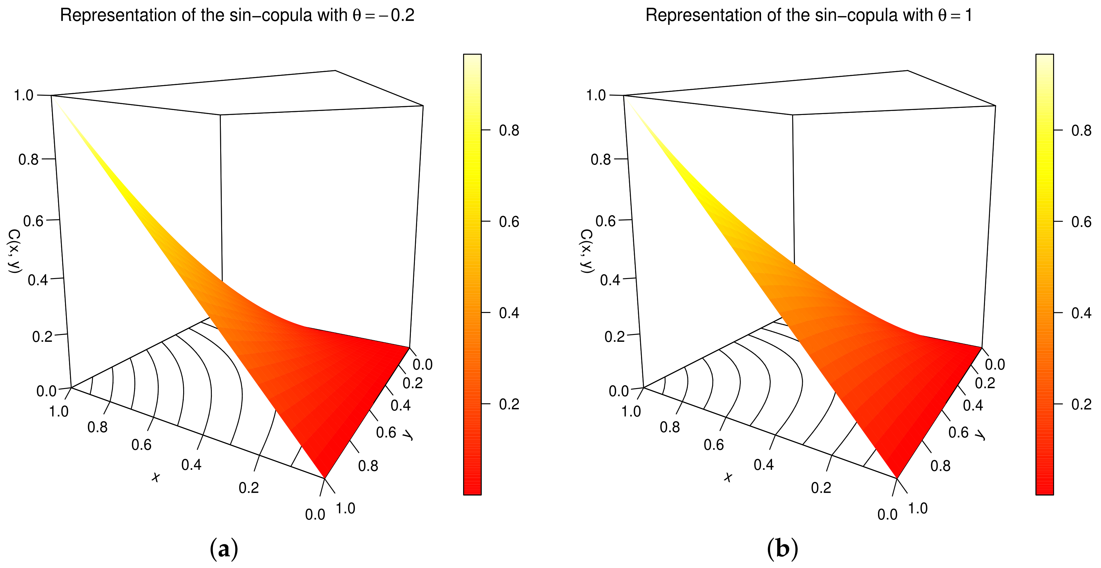
To end the presentation, Figure 8 represents the two-dimensional plot of the sin-copula for selected values of .
From Figure 8, we see that the parameter skews the triangular shape of the sin-copula.
The functions of the sin-copula, as well as its key features, are discussed in the following parts.
3.2. Related Functions
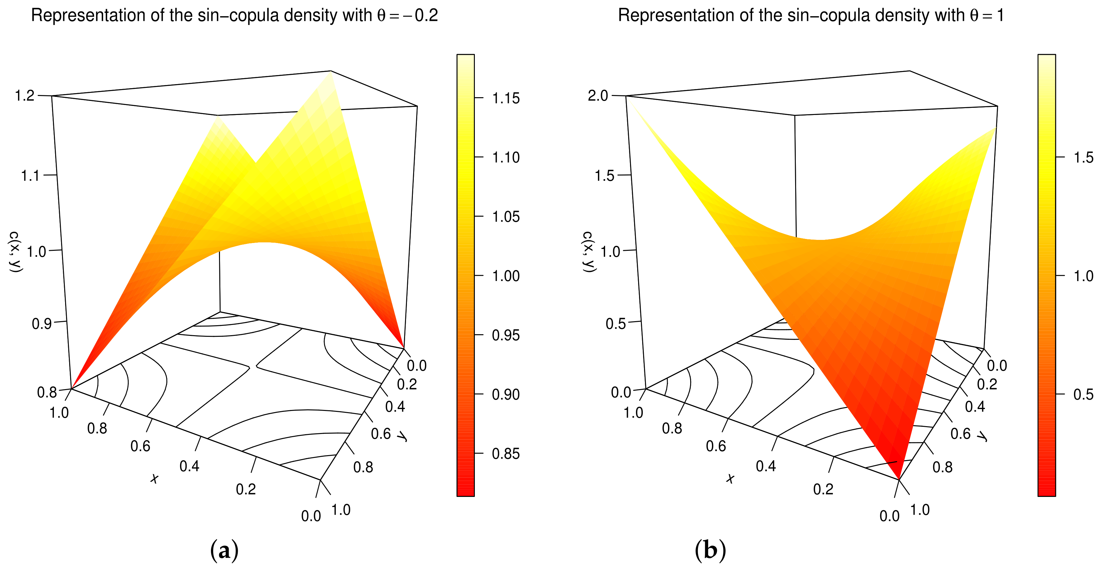
The density associated with the sin-copula is the function given by
It is worth noting that , which is negative for , and , which is negative for ; is not a copula for . In this sense, is the optimal set of values for .
Figure 9 represents the two-dimensional plot of the sin-copula density for selected values of .
As a result of Figure 9, we can see how influences the overall form of the sin-copula density.
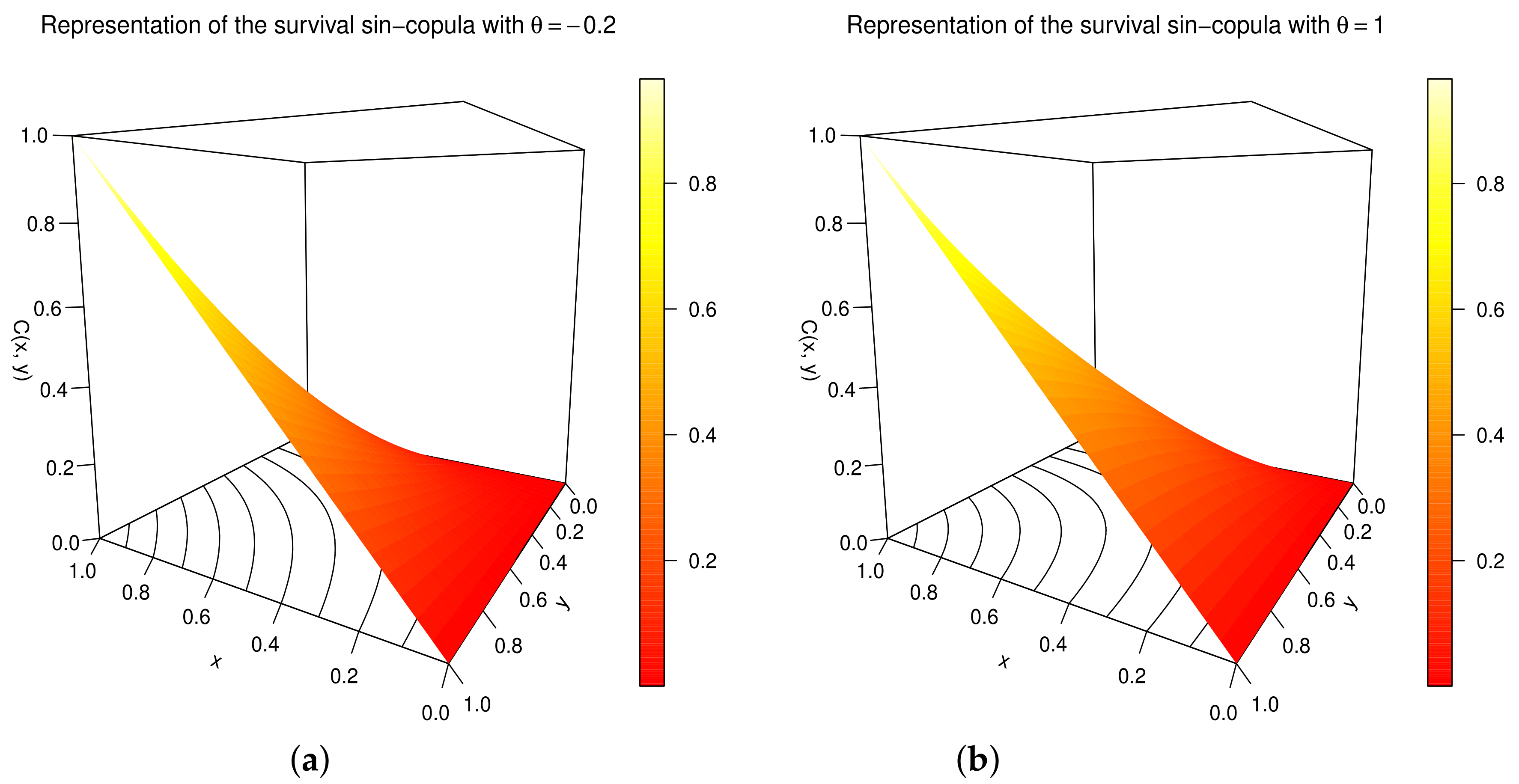
As a last important function, the survival sin-copula is the function defined by
It establishes a valid copula, which is also a new trigonometric copula with as an angle parameter.
Figure 10 represents the two-dimensional plot of the survival sin-copula for selected values of .
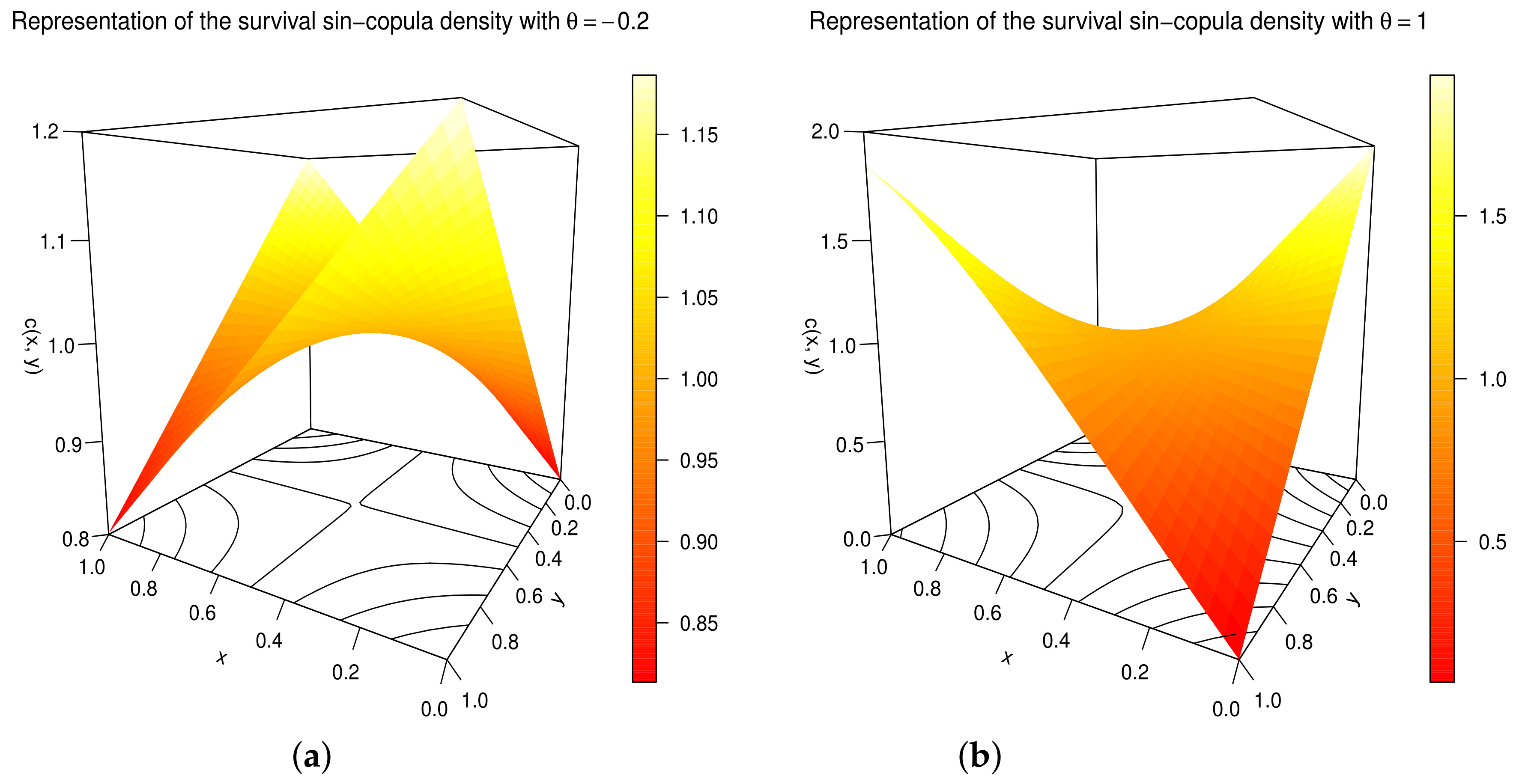
The copula density associated with the survival sin-copula is given by
To have an idea of its shapes, Figure 11 shows its two-dimensional plot for selected values of .
On the other hand, the sin-copula can be used in a variety of new mixed copulas. For instance, we can consider the following mixed sin-copulas:
- Mixed copula 1: For any angle parameters and , and , by setting , we can consider
- Mixed copula 2: Similarly, for any angle parameters and , and , by setting and , we can set
- Mixed copula 3: Another example is
They are also new angle parameter trigonometric copulas by construction.
3.3. Properties
The main features of the sin-copula as described in Equation (9) are now listed.
- As already mentioned before:
- –
- For , it is clear that . Therefore, the sin-copula is reduced to the independence copula.
- –
- The set is the optimal set of values for for validating as a copula.
- For any , we have , so the negative quadrant dependence property is satisfied. Similarly, for any , we have , so the positive quadrant dependence property is satisfied (see [21]).
- The sin-copula is symmetric since for any .
- The sin-copula can be expressed under various analytical forms. Two of them are given below:
- –
- In terms of simple cosine-sine functions, we can writeAs a result, we can observe that the sin-copula has inherent analytical complexity.
- –
- In terms of power series, by using the cosine series expansion and binomial formula, we getIn particular, upon differentiation with respect to x and y on the interior of the domain of convergence, one hasThis expansion can be used to determine various moment-type measurements in a range of mathematical applications.
- By arbitrary taking , we notice thatAs a result, the sin-copula is not Archimedean (see [1]).
- The sin-copula is not radially symmetric since there exists such that .
- As any copula, the Fréchet-Hoeffding bounds can be expressed as follows: For any , we have .
- Thanks to the inequality: and the Jordan inequality: for (see [20]), we have a copula ordering between the sin-copula and FGM copula:
- –
- For , we have
- –
- For , the contrary holds:
- The following relationship between the cos-copula and sin-copula holds:Therefore, the following ordering results are established:
- For any , the two following results are obtained:andHence, the sin-copula has no tail dependence.
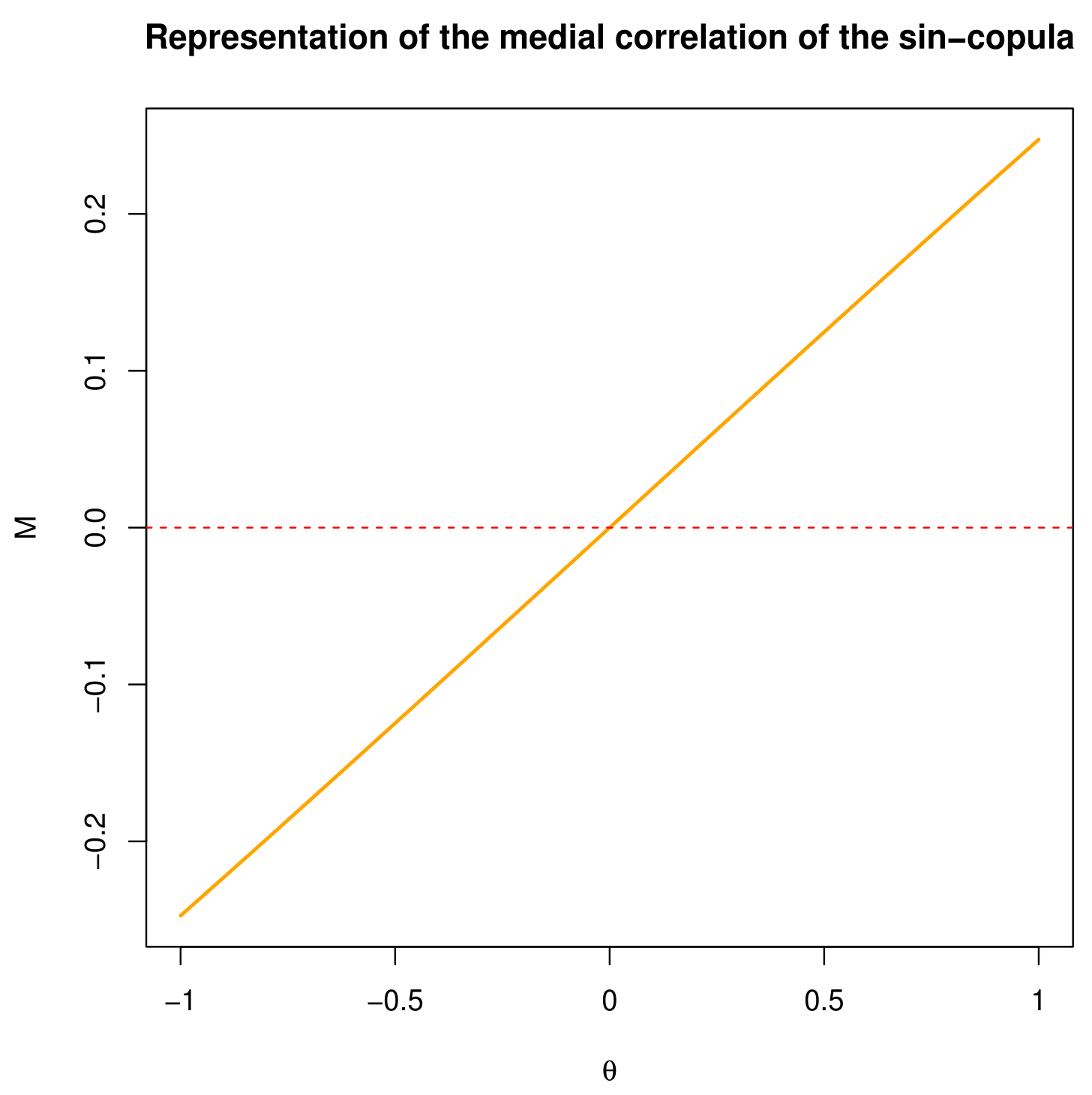
- The medial correlation of the sin-copula is defined byIt is clearly an increasing function with respect to for , with for and for . Figure 12 represents the medial correlation for .The possible values of this medial correlation are not negligible; we have . Hence, the sin-copula has a certain flexibility in this regard.
- The Spearman rho of the sin-copula, as an example of copula, is defined byUsing well-known mathematical methods, the following assertion provides a mathematical expression for this measure.
Proposition 4.
The Spearman rho of the sin-copula can be expressed as
Proof.
- For , we have and, by Equation (13), it is immediate that .
- For , still based on the definition of in Equation (13), we haveBy using a step-by-step integration, we obtainImmediately, the intended result occurs.
- For , thanks to the oddity of the sine function, we can writeSince , the expression of can be transposed with instead of , with the minus in factor of the overall expression.
The stated proposition is proved. □
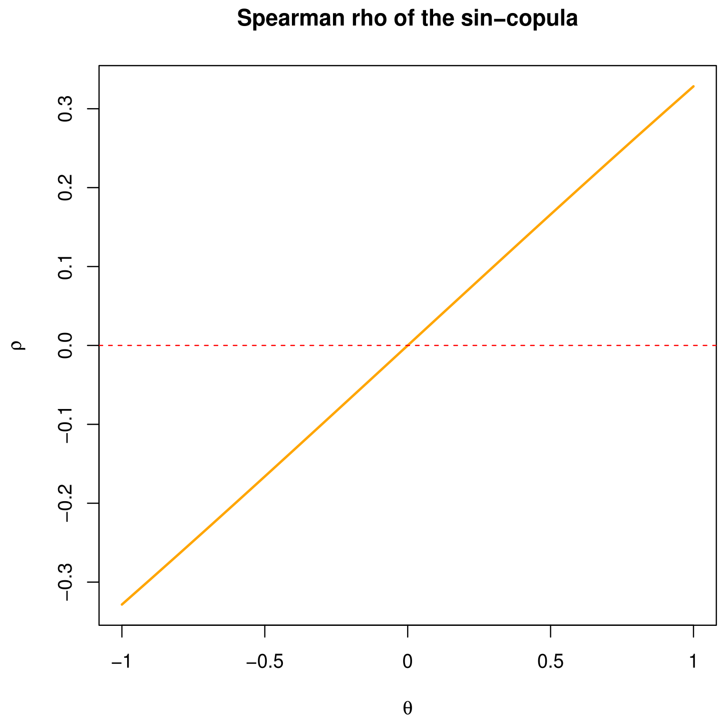
The measure is an increasing function with respect to for , with for , for , and for . Figure 13 represents the Spearman rho for .
In light of the above results, the sin-copula is adapted to model moderate correlations, which may be negative or positive.
Remark 3.
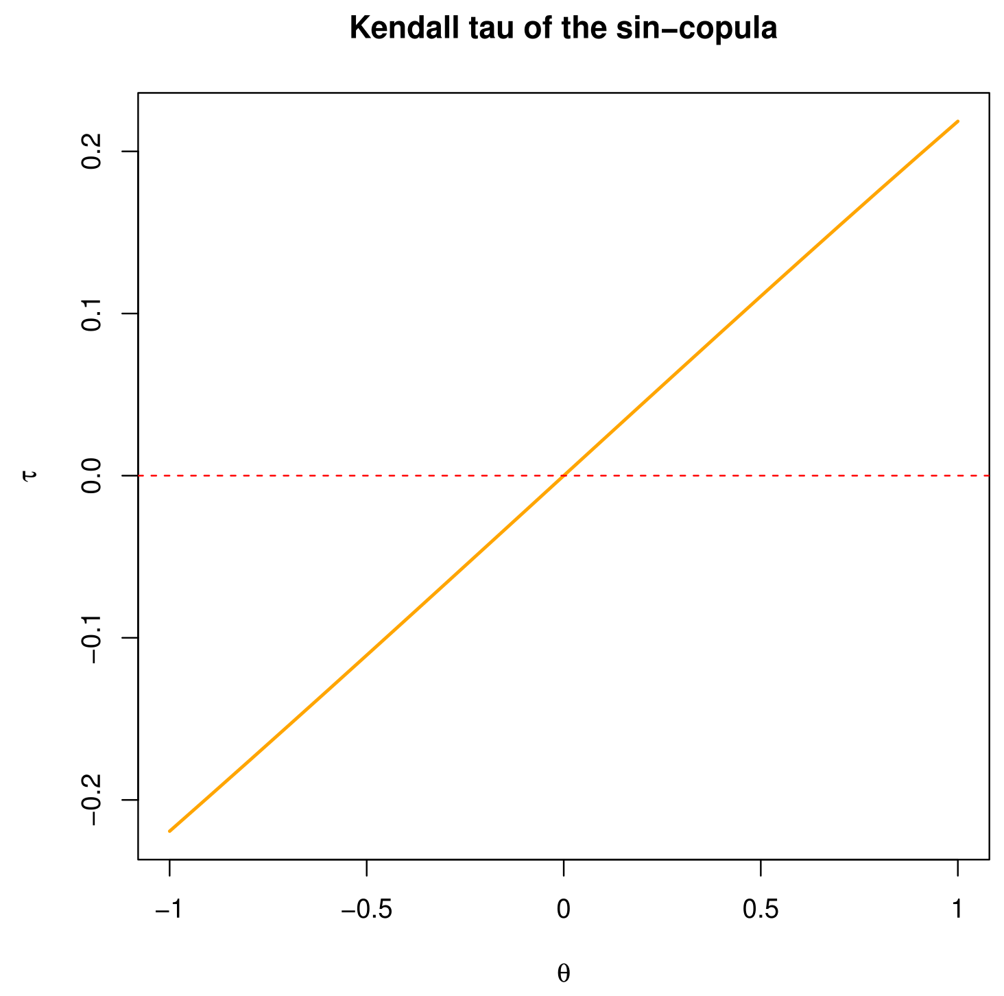
- In complement of the Spearman rho, we can present the Kendall tau of the sin-copula. It is defined byThe complexity of the product function makes the closed form expression for unmanageable. We can, however, show that it is an increasing function with respect to for , with for , for and for . Figure 14 represents the Kendall tau for .The wide range of values of confirm the fact that the sin-copula is ideal to model moderate correlations.
- Similarly to the cos-copula, the sin-copula opens up several fascinating possibilities, such as the development of simple and new two-dimensional distributions with cumulative distribution functions of the form: , sowhere and denote two cumulative distribution functions. As a result, probabilistic or statistical modeling in this context becomes more feasible.
3.4. Data Generation and Inference
The data generation method described in Section 2.4 can be configured for the sin-copula. For any positive integer n, we can generate n data from the sin-copula by proceeding as follows:
- Generate n data from a random vector , where S and T are independent random variables with the uniform distribution over .
- Choose a value for .
- Consider the following “conditional function”:
- For any , compute such that .
- Then are n data generated from the sin-copula defined with the chosen value of .
Other techniques are available (see [24]).
In a data analysis scenario, the angle parameter is usually unknown. Its estimation is thus useful for exact data fitting, or at the very least for determining if is close to 0, corresponding to the independent case, or close to or 1, corresponding to the most highly negatively or positively correlated situations, respectively. For this evaluation, it can be estimated from n data , that are susceptible to coming from the sin-copula distribution, by the maximum likelihood method; is thus estimated by
Concrete applications of the aforementioned methodologies to real-world datasets are thus possible.
4. Conclusions and Perspectives
4.1. Conclusions
We have introduced and studied several trigonometric copulas that have the features to depend on a tuning angle parameter. We have shown that they are quite simple from the mathematical point of view, and possess interesting properties.
For the first copula, called cos-copula, we have demonstrated that: (i) it extends the independence copula; (ii) it has the negative quadrant property; (iii) it is symmetric; (iv) it is not Archimedean; (v) it is not radially symmetric; (vi) a special ordering exists between it and the FGM copula; (vii) it has no tail dependence; (viii) the medial correlation belongs to the interval ; (ix) the Spearman rho belongs to the interval ; (x) the Kendall tau belongs to the interval ; (xi) it can serve to create a plethora of trigonometric two-dimensional distributions. Thus, the cos-copula is adapted to model weak negative correlations. It is thus not adapted to model moderate or large correlations. The corresponding copula density, survival copula, and survival copula density have been expressed, as well as two mixed copula versions.
For the second copula, called the sin-copula, its properties can be listed as follows: (i) it extends the independence copula; (ii) it has the negative and positive quadrant properties; (iii) it is symmetric; (iv) it is not Archimedean; (v) it is not radially symmetric; (vi) comprehensive ordering exists between it and both the FGM copula and cos-copula; (vii) it has no tail dependence; (viii) the medial correlation belongs to the interval ; (ix) the Spearman rho belongs to the interval ; (x) the Kendall tau belongs to the interval ; (xi) it can also serve to create a plethora of trigonometric two-dimensional distributions. Thus, the sin-copula is adapted to model moderate negative or positive correlations. The corresponding copula density, survival copula, and survival copula density have been expressed, as well as three mixed copula versions.
The shapes of the principal functions and their related features have been visually observed using graphics.
4.2. Perspectives
Thus, the first elements for the promotion of the proposed copulas are in this article. Perspectives of further research includes the following points:
- Following the spirit of some power-extended FGM copulas (see [25]), one can think of considering some extensions of the cos-copula and sin-copula of the forms:andrespectively, where , and c are newly introduced shape parameters. However, the possible values of , and c such that and are valid copulas remain to discover.
- The n-dimensional versions of the cos-copula and sin-copula, which can be defined as and , respectively, whereandrespectively, deserve to be investigated for . Especially, the possible values for in this case need to be determined.
- Last but not least, other simple angle parameter copulas can be created on the basis of this study. One could think of defined bybut the optimal values of such that is a valid copula remain unknown. It is proven that satisfies the required conditions (in an unpublished work), but this set is thought to be less than optimal.
Funding
This research received no external funding.
Acknowledgments
We thank the two reviewers and the associate editor for their in-depth comments on the first version of the article.
Conflicts of Interest
The author declares no conflict of interest.
References
- Nelsen, R. An Introduction to Copulas, 2nd ed.; Springer Science+Business Media, Inc.: Singapore, 2006. [Google Scholar]
- Durante, F.; Sempi, C. Principles of Copula Theory; CRS Press: Boca Raton, FL, USA, 2016. [Google Scholar]
- Emura, T.; Chen, Y.-H. Analysis of Survival Data with Dependent Censoring, Copula-Based Approaches; JSS Research Series in Statistics; Springer: Singapore, 2018. [Google Scholar]
- Joe, H. Dependence Modeling with Copulas; CRS Press: Boca Raton, FL, USA, 2015. [Google Scholar]
- Alfonsi, A.; Brigo, D. New families of copulas based on periodic functions. Commun. Stat.-Theory Methods 2005, 34, 1437–1447. [Google Scholar] [CrossRef] [Green Version]
- Amblard, C.; Girard, S. Symmetry and dependence properties within a semiparametric family of bivariate copulas. J. Nonparametr. Stat. 2002, 14, 715–727. [Google Scholar] [CrossRef] [Green Version]
- Chesneau, C. A study of the power-cosine copula. Open J. Math. Anal. 2021, 5, 85–97. [Google Scholar] [CrossRef]
- Chesneau, C. On new types of multivariate trigonometric copulas. Appl. Math. 2021, 1, 3–17. [Google Scholar] [CrossRef]
- Chesneau, C. A note on a simple polynomial-sine copula. Asian J. Math. Appl. 2022, 2, 1–14. [Google Scholar]
- Durante, F. A new class of symmetric bivariate copulas. J. Nonparametr. Stat. 2006, 18, 499–510. [Google Scholar] [CrossRef]
- Jones, M.C.; Pewsey, A.; Kato, S. On a class of circulas: Copulas for circular distributions. Ann. Inst. Stat. Math. 2015, 67, 843–862. [Google Scholar] [CrossRef]
- Davy, M.; Doucet, A. Copulas: A new insight into positive time-frequency distributions. IEEE Signal Process. Lett. 2003, 10, 215–218. [Google Scholar] [CrossRef]
- Hodel, F.H.; Fieberg, J.R. Circular-linear copulae for animal movement data. bioRxiv 2021. [Google Scholar] [CrossRef]
- Knockaert, L. A class of positive isentropic time-frequency distributions. IEEE Signal Process. Lett. 2002, 9, 22–25. [Google Scholar] [CrossRef] [Green Version]
- Susam, S.O. A new family of archimedean copula via trigonometric generator function. Gazi Univ. J. Sci. 2020, 33, 795–802. [Google Scholar] [CrossRef]
- Xiao, Q.; Zhou, S.W. Modeling correlated wind speeds by trigonometric Archimedean copulas. In Proceedings of the 11th International Conference on Modelling, Identification and Control (ICMIC2019); Lecture Notes in Electrical Engineering; Wang, R., Chen, Z., Zhang, W., Zhu, Q., Eds.; Springer: Singapore, 2020; Volume 582. [Google Scholar]
- Hodel, F.H.; Fieberg, J.R. Cylcop: An R package for circular-linear copulae with angular symmetry. bioRxiv 2021. [Google Scholar] [CrossRef]
- Manstavičius, M.; Bagdonas, G. A class of bivariate independence copula transformations. Fuzzy Sets Syst. 2021, 428, 58–79. [Google Scholar] [CrossRef]
- Kober, H. Approximation by integral functions in the complex domain. Trans. Am. Math. Soc. 1944, 56, 7–31. [Google Scholar] [CrossRef] [Green Version]
- Qi, F.; Hao, Q.-D. Refinements and sharpenings of Jordan’s and Kober’s inequality. Math. Inform. Q. 1998, 8, 116–120. [Google Scholar]
- Lehmann, E.L. Some concepts of dependence. Ann. Math. Stat. 1966, 37, 1137–1153. [Google Scholar] [CrossRef]
- Chesneau, C.; Artault, A. On a comparative study on some trigonometric classes of distributions by the analysis of practical data sets. J. Nonlinear Model. Anal. 2021, 3, 225–262. [Google Scholar]
- Tomy, L.; Satish, G. A review study on trigonometric transformations of statistical distributions. Biomet. Biostat. Int. J. 2021, 10, 130–136. [Google Scholar]
- Johnson, M.E. Multivariate Statistical Simulation; J. Wiley & Sons: New York, NY, USA, 1987. [Google Scholar]
- Bairamov, I.; Kotz, S. Dependence structure and symmetry of Huang-Kotz FGM distributions and their extensions. Metrika 2002, 56, 55–72. [Google Scholar] [CrossRef]
Figure 1.
Representations of the cos-copula for (a) and (b) .

Figure 2.
Representations of the cos-copula density for (a) and (b) .

Figure 3.
Representations of the survival cos-copula for (a) and (b) .

Figure 4.
Representations of the survival cos-copula density for (a) and (b) .

Figure 5.
Representation of the medial correlation of the cos-copula for .

Figure 6.
Representation of the Spearman rho of the cos-copula for .

Figure 7.
Representation of the Kendall tau of the cos-copula for .

Figure 8.
Representations of the sin-copula for (a) and (b) .

Figure 9.
Representations of the sin-copula density for (a) and (b) .

Figure 10.
Representations of the survival sin-copula for (a) and (b) .

Figure 11.
Representations of the survival sin-copula density for (a) and (b) .

Figure 12.
Representation of the medial correlation of the sin-copula for .

Figure 13.
Representation of the Spearman rho of the sin-copula for .

Figure 14.
Representation of the Kendall tau of the sin-copula for .

Publisher’s Note: MDPI stays neutral with regard to jurisdictional claims in published maps and institutional affiliations. |
© 2022 by the author. Licensee MDPI, Basel, Switzerland. This article is an open access article distributed under the terms and conditions of the Creative Commons Attribution (CC BY) license (https://creativecommons.org/licenses/by/4.0/).
Share and Cite
MDPI and ACS Style
Chesneau, C. Theoretical Study of Some Angle Parameter Trigonometric Copulas. Modelling 2022, 3, 140-163. https://doi.org/10.3390/modelling3010010
AMA Style
Chesneau C. Theoretical Study of Some Angle Parameter Trigonometric Copulas. Modelling. 2022; 3(1):140-163. https://doi.org/10.3390/modelling3010010
Chicago/Turabian StyleChesneau, Christophe. 2022. "Theoretical Study of Some Angle Parameter Trigonometric Copulas" Modelling 3, no. 1: 140-163. https://doi.org/10.3390/modelling3010010