Modelling of Biotrickling Filters for Treatment of NO_x Analytical Expressions for the NO_x Concentration in Both Gas and Biofilm Phases

Abstract

A mathematical model of an ideal biotrickling filter (BF) system that inoculates a recently identified strain of Chelatococcus daeguensis TAD1 and brings about efficient nitrogen oxide treatment is discussed. The proposed model is based on nonlinear mass transport equations at the gas–biofilm interface. Using Akbari–Ganji’s technique, approximate analytical expressions for the nitric oxide concentration in the gaseous and biofilm phases were developed for all feasible system parameters. In addition, to investigate the dynamic behaviour of the system, a numerical analysis of the problem is provided using MATLAB tools. To demonstrate this new approach, graphical data are provided and quantitatively discussed. This theoretical result has good agreement with the numerical simulation (MATLAB) results for the experimental values of parameters.

1. Introduction

In biotrickling filters, the biological treatment of contaminated air requires a complex combination of physical, chemical, and biological processes. It can be challenging to predict how biotrickling filters will behave under various conditions. Fortunately, computers and mathematical models are far more capable than the human mind at tracking many complex relationships. Mathematical models of biotrickling filtration can thus be beneficial in research and design. Additionally, these models facilitate the creation of a basic understanding of the process and technical tasks, such as reactor design, scaleup, and process optimization [1].

The modelling process implies some translation of concepts into equations that can be solved. In most cases, the modelling of biotrickling filters involves mass balances of the contaminant(s), oxygen, and products resulting from contaminant degradation. These include the gas phase, a solid phase, and biofilm and liquid phases in the case of biotrickling filters. Depending on the model concept and assumptions, the resulting equations may include terms for the accumulation of reactive products (i.e., odours, VOCs, oxygen, nitrogen oxide, nutrients, and by-products) in all phases, dispersion effects in air, mass transfer between the air and biofilm phases, diffusional mass transfer in the biofilm, consumption due to biological oxidation, adsorption onto solid media, biomass growth, the physiological state of the biomass, etc. [1]. Thus, the resulting model often comprises a complex set of nonlinear partial differential equations with initial and boundary conditions. Most of the time, exact analytical solutions are difficult or impossible, and methods are used with the appropriate numerical algorithms to obtain solutions to the model instead.

More recently, Kalandar et al. [2] developed a comprehensive dynamic mathematical model consisting of mass transfer through gas, liquid, and biofilm phases with the kinetics of biodegradation in the BTF and accumulation of methanol in the liquid. A mathematical model for the simulation of the removal of hydrophilic compounds using biotrickling filtration was developed by San-Valero [3].

Biotrickling filters can effectively be used in NO removal. Many researchers have used the process to treat nitrogen oxide (NOx)-contaminated gas via denitrification [4,5]. The emission of nitrogen oxides (NOx) and their induced secondary contaminants is harmful to human health [6]. Breathing air with a high nitrogen oxide concentration can irritate the human respiratory system’s airways. Short-term exposure can increase respiratory diseases, such as asthma, coughing, wheezing, and difficulty breathing. NO₂ and other NOx species react with other chemicals in the air to form ozone, which is harmful when inhaled due to its effects on the respiratory system. NOx interacts with the atmosphere’s water, oxygen, and other chemicals to form acid rain. Acid rain has a negative impact on sensitive ecosystems, such as lakes and forests. The presence of nitrogen oxides in the atmosphere adds to nutrient contamination in coastal waters.

Because NOx pollution has such a negative impact on the environment and human health, it must be strictly controlled. This involves the implementation of cost-effective removal strategies that simultaneously create value-added by-products or energy from the waste. NOx emissions from various industrial activities and transportation operations, especially coal-fired energy plants, are widely acknowledged as hazards to the environment and human well-being [7]. Since combustion process control can significantly reduce NOx emissions, the treatment of exhaust gases from post-combustion is essential to meet today’s statutory air standards [8]. New post-combustion control technologies, such as biotrickling filters (BTFs), could be used to purify NOx-containing dilute gases [9,10].

According to Ligy and Marc], within a biotrickling filter, nitrogen oxide is converted to nitrogen gas under anoxic conditions by chemolithoautotrophic organisms [11]. To resolve this problem, a small number of researchers have worked on isolating thermophilic microorganisms to remove NOx, which may offer greater savings and significantly expand the application of BTFs. Jiang et al. [12] described an effective biotrickling filter system for removing nitric oxide from flue gas using Pseudomonas putida. Liang et al. [13] designed a mathematical model for the elimination of nitric oxide in a thermophilic biotrickling filter. No comprehensive analytical expressions of the nitric oxide concentration in the gas or biofilm phases have been published yet.

Flanagan and Lee [14,15] investigated the reduction of NO by using thermophilic microorganisms at various temperatures. Furthermore, due to the non-linear nature of mass balance equations over the biofilm phase, theoretical modelling studies on NO removal in BTF reactors are limited. Caceres, Song, and Zarook developed theoretical BTF modelling for the removal of volatile organic compounds [16,17,18]. Under thermophilic circumstances, Liang et al. [13] developed a mathematical model for nitrogen oxide removal in a biotrickling filter. Meena et al. [19,20] discussed mathematical models of the biofiltration of mixtures of hydrophilic (methanol) and hydrophobic (α-pinene) volatile organic compounds (VOCs) in biofilters.

However, to the best of our knowledge, no exact analytical expressions of the nitrogen oxide concentration in the gas and biofilm phases have been reported [13]. The aim of this study is to generate approximate analytical results for the nitrogen oxide concentration in both the gas and biofilm phases using Akbari–Ganji’s method. This result will be beneficial in optimizing the key parameters for the efficiency of nitrogen oxide removal from air pollutants by biotrickling filters.

2. Mathematical Formulation of the Problem

A theoretical model of a modern BTF reactor packed with homogenous ceramic particles will now be discussed. This is based on the work reported initially by Liang and co-workers [13]. We briefly describe the principles of a typical experimental biotrickling filter system (refer to Figure 1 of [13]) in order to place the mathematical model in context [13]. Typically, a mass flow controller is used to control the flow of NO, N₂, and O₂ in the experiment with continuous gas streams for the thermophilic removal of NO. A flue gas analyser is used to measure the entry and exit amounts of NO, NO₂, and O₂. The water flow rate through the flow cells is controlled by recirculating the water by means of recirculation pumps. No free liquid is recirculated through the packing materials, and the nutrient liquid is continuously supplied using a top sprayer to minimize the effect of nutrient limitation on biofilm growth. A top sprayer is used to continuously provide the nutrient liquid. As a result, the total BTF operations can be considered in two phases: gas and biofilm, which are connected by a thin interfacial film.

The following assumptions must be included to develop the mass balance equations for both phases [21,22]:

• The biofilm can be perceived as a planar surface owing to the radius of the packing particles, which is comparatively larger than the biofilm’s thickness; the gas flows through the crammed layer in a parallel pattern through a series of vertical channels;
• The gas phase is moved in a plug flow manner, with no consideration for axial diffusion. Molecule diffusion is used to transport NO in biofilms;
• The rate-limiting substrate is NO. Therefore, there is no depletion of oxygen or nutrients. It has been proven that the amount of oxygen in the environment is considered in excess, and hence the reaction of NO and molecular oxygen is pseudo-second-order in terms of the NO concentration;
• The consistent properties of the biofilm across the reactor and negligible biomass production in the packing materials result in a stable value of the biofilm kinetic constants. Here, the biofilm growth is depicted by Monod growth kinetics;
• Inside the biofilm, only one direction of diffusion/reaction occurs, which is perpendicular to the gas–biofilm boundary. Oxygen in the gas phase influences the partial oxidation of NO to NO₂ and swiftly forms nitrates or nitrates by dissolving in water;
• Because of oxygen in the gas phase, NO is partially oxidized to NO₂ and quickly dissolved in water to yield nitrite or nitrate. This portion of nitric oxide that has been converted to aqueous nitrogen compounds will not return to the gas phase, so it can be considered to be removed from the gas phase. In fact, nitrite or nitrate in water could be rapidly denitrified to N₂ by denitrifiers.

In Figure 1, we present a schematic representation of the concentration profile of NO_x in the gas and biofilm phases indicating the coordinate systems used and their relation to one another. The concentration profiles refer to a single particle in the biofilter covered with a uniform layer of biofilm of thickness $L_f$.

2.1. Mass Balance in the Gas Phase

On the basis of the above assumptions, the mass balance equations in the gas and biofilm phase are given as follows.

$$U_g\frac{d{C}_g}{dz}=-J_{f,o}{a}_f-r_c{\epsilon }_f$$

(1)

where $J_{f,0}$ represents the diffusion flux at the position where $x=0$, i.e., the flux across the gas/biofilm interface (unit: gcm⁻² s⁻¹). Furthermore, $a_f$ denotes the specific surface area (surface area/mass) of the biofilm (unit: cm⁻¹), and $r_c$ denotes the gaseous chemical reaction velocity (unit: g cm⁻³ s⁻¹). Noting assumption 6, this gas-phase reaction of NO with molecular oxygen involves the process 2NO + O₂ → 2NO₂, which is rate-determining, and so the rate term is bimolecular and of the type $r_c=2k_g{C}_g{}^2$, where we have assumed that oxygen is present in great excess. According to the Fick law, the diffusion flux is related to the concentration gradient at the gas/biofilm interface by the following expression:

$$J_{f,0}=-D_e{\left(\frac{d{C}_{\ell }}{dx}\right)}_{x=0}$$

(2)

Hence, the mass balance at x = 0 transforms to:

$$U_g\frac{d{C}_g}{dz}=a_f{D}_e{\left(\frac{d{C}_{\ell }}{dx}\right)}_{x=0}-2k_g{C}_g{}^2$$

(3)

Note that the initial condition governing this differential equation is given by

$$z=0\hspace{1em}{C}_g=C_{g,0}$$

(4)

where $C_g \mathrm{and} C_l$ stand for the gas and biofilm phase $\mathrm{NO}$ concentrations, $U_g$ is the superficial gas velocity, $a_{f }$is the surface area of biofilm, $D_e$ denotes the effective diffusion coefficient of NO within the biofilm phase, $k_g$is the bimolecular reaction rate constant, and ${\epsilon }_f$ denotes the biofilm porosity ratio. We note that $x$ represents the coordinate axis calculated from the surface of the biofilm and whose direction is perpendicular to the surface of the biofilm-coated particle. Furthermore, we note that the variable $z$denotes the height from the bottom of the packing materials and so defines a coordinate representing the length of the biofiltration column.

2.2. Mass Balance Equation in the Biofilm Phase

The expression for the mass balance in the biofilm phase is given by the balance between the molecular diffusion of NO through the liquid phase and the reaction kinetics by which the NO substrate of concentration $C_{\ell }$ is transformed by immobilized micro-organisms according to Monod kinetics:

$$D_e\frac{d^2{C}_{\ell }}{d{x}^2}=\frac{{\mu }_m}{Y}\frac{C_{\ell }}{K_S+C_{\ell }}{X}_V$$

(5)

where ${\mu }_m$ is the maximum specific biomass growth rate, $Y$ is the yield coefficient of micro-organisms, ${\mu }_m/Y$ gives the maximum specific substrate utilization rate, $K_S$ is the Monod half-saturation constant, $X_V$ is the biofilm microbial density, $H$ is Henry constant at a fixed temperature, and $L_f$ is the biofilm thickness.

The boundary conditions governing the reaction diffusion equation in the biofilm are given by

$$\mathrm{At} x=0, C_{\ell }\left(x=0\right)=\frac{C_g}{H}$$

(6)

$$\mathrm{At} x=L_F, \frac{d{C}_{\ell }}{dx}=0$$

(7)

The first boundary condition specifies the partitioning of the NO species from the gas phase to the liquid biofilm and H represents the gas/liquid Henry volatility constant for temperature T. This value decreases as the gas solubility increases. The second condition relates to a zero-flux condition and the biofilm/solid particulate support interface, since the support particle is assumed to be inert.

2.3. Dimensionless Form

The problem may be expressed in an efficient format by defining the following dimensionless parameters that involve scaling the NO concentration and introducing normalized distance parameters, a saturation parameter, a reaction/diffusion parameter, and parameters comparing molecular diffusion with gas velocity and gas-phase chemical reaction with the superficial gas velocity, as follows:

$${\overline{C}}_{\ell }\left(\overline{x}\right)=\frac{C_{\ell }}{ C_{g/H} }, \overline{x}=\frac{x}{L_F} \alpha =L_F\sqrt{\frac{{\mu }_m{X}_V}{Y{D}_e{K}_S}}, \beta =\frac{C_{g/H}}{K_S}$$

(8)

$${\overline{C}}_g\left(\overline{z}\right)=\frac{C_g\left(z\right)}{C_{g,0}}\hspace{0.17em}, \overline{z}=\frac{z}{L_F}, \gamma =\frac{a_F{D}_e}{U_{g}H}, \eta =\frac{{\epsilon }_f{k}_g{C}_{g,0}{L}_F}{U_g}$$

(9)

We can readily show that Equation (5) reduces to the following normalized form with the corresponding boundary conditions as follows:

$$\frac{d^2{\overline{C}}_{\ell }}{d{\overline{x}}^2}-\frac{{\alpha }^2{\overline{C}}_{\ell }}{1+\beta {\overline{C}}_{\ell }}=0$$

(10)

$${\overline{C}}_{\ell }\left(\overline{x}=0\right)=1$$

(11)

$${\left(\frac{d{\overline{C}}_{\ell }}{d\overline{x}}\right)}_{\overline{x}=1}=0$$

(12)

Note that Equation (10) is a non-linear differential equation describing molecular diffusion and Monod kinetics within the thin biofilm. We assume that the biofilm thickness is much smaller than the radius of the support particle, and so the geometry of the reaction/diffusion problem is assumed to be planar without serious error. Furthermore, Equation (1) describing the mass balance at the gas/biofilm phase boundary is converted to the normalized form as shown below:

$$\frac{d{\overline{C}}_g}{d\overline{z}}-\gamma {\overline{C}}_g{\left(\frac{d{\overline{C}}_{\ell }}{d\overline{x}}\right)}_{\overline{x}=0}+2\eta {\overline{C}}_g{}^2=0$$

(13)

$${\overline{C}}_g\left(\overline{z}=0\right)=1$$

(14)

We note that Equation (10) is nonlinear. As outlined in Appendix A, we show that this non-linear first-order differential equation for the NO concentration in the gas phase is of the Bernoulli type and may be transformed into a first-order linear differential equation by means of a simple substitution. We now discuss how an efficient approximate analytical solution to these coupled nonlinear differential equations may be solved using the Akbari–Ganji method (AGM).

3. Approximate Analytical Expression of the Concentration Using the Akbari–Ganji Method

Nowadays, many analytical methods are available for solving nonlinear differential equations [23,24,25,26,27,28,29,30,31]. Such methods include the Akbari–Ganji method [32,33,34,35], domain decomposition method [36,37], homotopy perturbation method [38,39,40,41], Taylor’s series method [42,43,44], variational iteration method [45], and Padé approximant method [46].

One of the most successful methods for solving nonlinear differential equations is the AGM method. AGM has a very simple approach to solving a differential equation as compared with other semi-analytical techniques, requiring only the initial/boundary conditions, the main differential equations, and their derivatives. In this study, this method is used for the first time to derive analytical expressions for the NO concentration both in the gas and biofilm phases of a biotrickling filter.

As presented in Appendix A, we can show that the Akbari–Ganji technique can be used to derive an analytical expression for the NO concentration in the biofilm phase $\overline{C_l}\left(\overline{x}\right)$ for all values of the dimensionless reaction/diffusion parameter $\alpha$ and the binding/saturation parameter $\beta$ as follows:

$${\overline{C}}_{\ell }\left(\overline{x}\right)=\frac{\cosh \left[\frac{\alpha }{\sqrt{1+\beta }}\left(1-\overline{x}\right)\right]}{\cosh \left[\frac{\alpha }{\sqrt{1+\beta }}\right]}=\mathrm{sech}\left[\frac{\alpha }{\sqrt{1+\beta }}\right]\cosh \left[\frac{\alpha }{\sqrt{1+\beta }}\left(1-\overline{x}\right)\right]$$

(15)

Furthermore, we show in Appendix B that an analytical expression for the NO concentration in the gas phase is given by the following expression:

$$C_g\left(\overline{z}\right)=n{\left\{(\mathit{exp}\left[n\overline{z}\right]\left(n+2\eta \right))-2\eta \right\}}^{-1}$$

(16)

where the parameter $n$ is related to the flux of NO through the biofilm and is given by the following expression:

$$n=-\gamma {\overline{C}}_{\ell }^{\prime }\left(\overline{x}=0\right)$$

(17)

Furthermore, we note that the differentiation of Equation (15) enables us to compute a simple closed-form value for the NO flux in the biofilm phase, which is given by:

$$J_0=-{\left(\frac{d{\overline{C}}_{\ell }\left(\overline{x}\right)}{d\overline{x}}\right)}_{\overline{x}=0}=\frac{\alpha }{\sqrt{1+\beta }}\mathit{tanh}\left[\frac{\alpha }{\sqrt{1+\beta }}\right]$$

(18)

This expression for the flux of NO through the biofilm can be related in a simple manner to the degree of saturation of Monod kinetics in the film and the rate of molecular diffusion to NO utilization by the immobilized microbe species in the layer. From Equations (17) and (18), we can show that:

$$n=\frac{\alpha \gamma }{\sqrt{1+\beta }}\mathit{tanh}\left[\frac{\alpha }{\sqrt{1+\beta }}\right]$$

(19)

Hence, Equations (14) and (15) define the desired relation between the concentration of NO in the gas phase and the flux of NO in the biofilm phase. From Equations (10) and (13), we obtain the following expression for the NO concentration in the gas phase:

$$C_g\left(\overline{z}\right)=\frac{\frac{\alpha \gamma }{\sqrt{1+\beta }}\mathit{tanh}\left[\frac{\alpha }{\sqrt{1+\beta }}\right]}{\mathit{exp}\left(\frac{\alpha \gamma }{\sqrt{1+\beta }}\mathit{tanh}\left[\frac{\alpha }{\sqrt{1+\beta }}\right]\hspace{0.17em}\overline{z}\right)\left(\frac{\alpha \gamma }{\sqrt{1+\beta }}\mathit{tanh}\left[\frac{\alpha }{\sqrt{1+\beta }}\right]+2\eta \right)-2\eta }$$

(20)

Hence, we have derived two closed-form expressions for the NO concentration in both the gas and biofilm phases that are in good agreement with the numerical solution over a wide range of parameters, as indicated later in this paper.

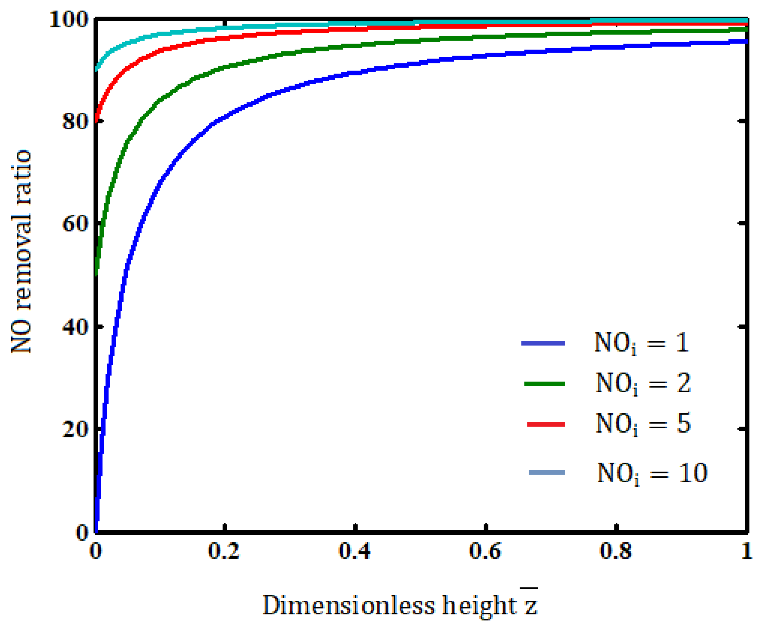
4. Removal Efficiency of Nitric Oxide

The $\mathrm{NO}$ absorption ratio or $\mathrm{NO}$ removal efficiency is expressed as follows [42]:

$$RE=\frac{{\left[\mathrm{NO}\right]}_i-{\left[\mathrm{NO}\right]}_f}{{\left[\mathrm{NO}\right]}_i}=1-\frac{{\left[\mathrm{NO}\right]}_f}{{[\mathrm{NO}]}_i}=1-\frac{{\overline{C}}_g(\overline{z})}{{[\mathrm{NO}]}_i}$$

(21)

where $\mathrm{N}{\mathrm{O}}_i$ and $\mathrm{N}{\mathrm{O}}_f$ represent the initial (pre-treatment) and the final (post-treatment) $\mathrm{N}\mathrm{O}$ concentrations in the gas phase.

5. Previous Analytical Results

It is useful to compare the AGM-derived expressions outlined in Equations (15) and (20) for the NO concentration with analytical expressions derived using different methods. Rasi et al. [36] used the Adomian decomposition method (ADM) to solve Equations (10) and (13) with the associated boundary conditions used in the present paper. Their analytical expressions for the $\mathrm{NO}$concentration of the biofilm and gas phases are, respectively, given by

$${\overline{C}}_{\ell }\left(\overline{x}\right)=1-\frac{{\alpha }^2\overline{x}}{2\left(1+\beta \right)}\left\{2-\overline{x}-\frac{{\alpha }^2\left({\overline{x}}^2\left(\overline{x}-4\right)+8\right)}{12{\left(1+\beta \right)}^2}\right\}$$

(22)

and

$${\overline{C}}_g\left(\overline{z}\right)=\frac{\gamma m}{\mathit{exp}\left[\gamma m\overline{z}\right]\left(\gamma m+2\eta \right)-2\eta }$$

(23)

where

$$m=\frac{{\alpha }^2}{1+\beta }\left\{\frac{{\alpha }^2}{3{\left(1+\beta \right)}^2}-1\right\}$$

(24)

These expressions are also very useful for numerical computation.

6. Numerical Simulation

The non-linear reaction/diffusion equation in the biofilm phase outlined in Equation (15) is solved numerically for the relevant boundary conditions. As outlined in Appendix C, the MATLAB function bvp4c is used to solve this equation, which is a function for solving two-point boundary value problems for nonlinear differential equations. These numerical solutions were then compared with the approximate closed-form analytical solutions derived via the AGM to probe the accuracy of the latter.

Consequently, in

Table 1. Comparison between numerical and analytical results for the dimensionless $\mathrm{NO}$ concentration of the biofilm phase ${\overline{c}}_l\left(\overline{x}\right)$ for various values of parameter $\alpha$ when $\beta =0.01$.

$\overline{\mathit{x}}$	$\mathit{\alpha } \mathbf{=} \mathbf{0.01}$					$\mathit{\alpha } \mathbf{=} \mathbf{0.5}$					$\mathit{\alpha } \mathbf{=} \mathbf{1}$
	Num.	Concentration in Biofim Phase		Error (%)		Num.	Concentration in Biofim Phase		Error (%)		Num.	Concentration in Biofim Phase		Error (%)
		This Work AGM Equation (15)	ADM [31] Equation (22)	This Work AGM Equation (15)	ADM [31] Equation (22)		This Work AGM Equation (15)	ADM [31] Equation (22)	This Work AGM Equation (15)	ADM [31] Equation (22)		This Work AGM Equation (15)	ADM [31] Equation (22)	AGM Equation (15)	ADM [31] Equation (22)
0	1.0000	1.0000	1.0000	0.00	0.00	1.0000	1.0000	1.0000	0.00	0.00	1.0000	1.0000	1.0000	0.00	0.00
0.2	0.9982	0.9982	0.9982	0.00	0.00	0.9587	0.9587	0.9591	0.00	0.04	0.8663	0.8666	0.8843	0.03	2.07
0.4	0.9968	0.9968	0.9968	0.00	0.00	0.9271	0.9271	0.9278	0.00	0.08	0.7678	0.7683	0.8019	0.06	4.44
0.6	0.9958	0.9958	0.9958	0.00	0.00	0.9049	0.9049	0.9058	0.00	0.09	0.7005	0.7011	0.7473	0.08	6.68
0.8	0.9953	0.9953	0.9953	0.00	0.00	0.8918	0.8918	0.8929	0.01	0.12	0.6617	0.6624	0.7165	0.11	8.28
1	0.9951	0.9951	0.9951	0.00	0.00	0.8877	0.8877	0.8889	0.01	0.13	0.6498	0.6605	0.7072	0.11	8.83
	Average error %			0.00	0.00	Average error %			0.01	0.08	Average error %			0.06	5.05

and Figure 2, Figure 3 and Figure 4, the analytical results for the NO concentration were compared with simulation data and previously available analytical results (obtained using ADM). The maximum average error between our new analytical result (obtained using the AGM method) and the simulation result was 0.64%. In comparison, the previous analytical result (obtained via the ADM method) and the simulation result had a maximum average error of 5.05%. Therefore, we conclude that the ADM method has a prolonged convergence rate and the AGM provides a better fit for simulation predictions. The AGM method is also attractive since it enables the development of a closed-form analytical solution to a non-linear reaction/diffusion equation that can be computed readily, and can be readily interpreted in terms of the degree of utilization of the biofilm in the consumption of the target substrate.

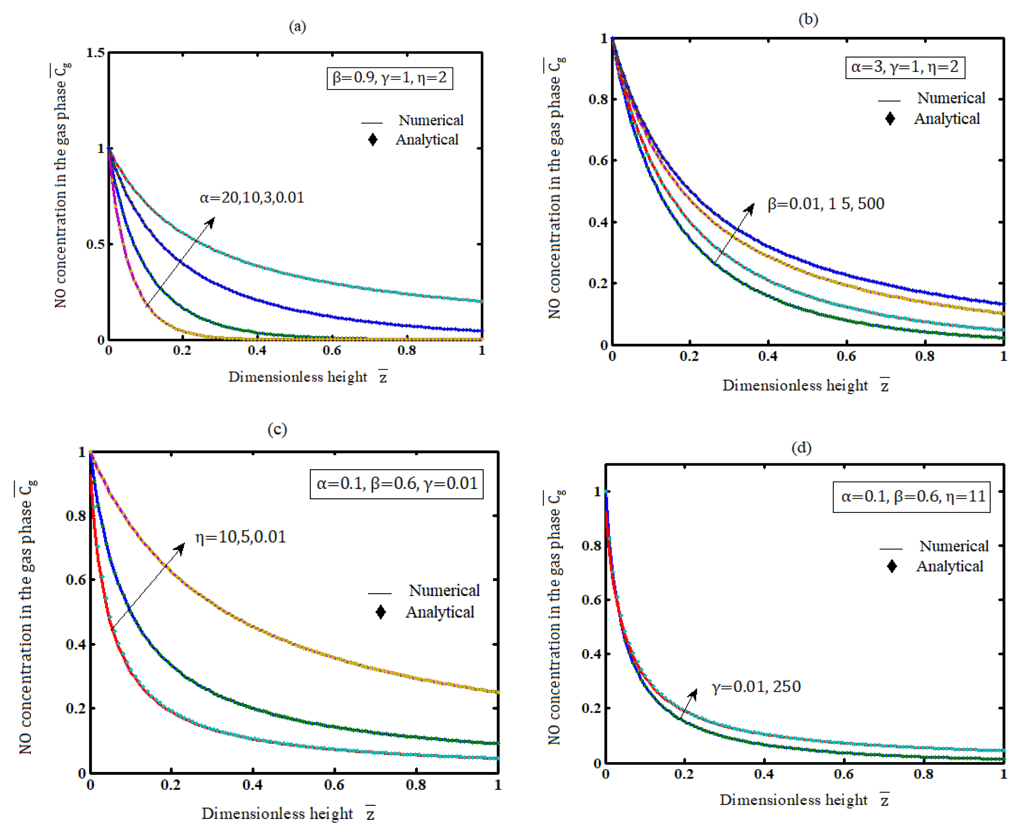
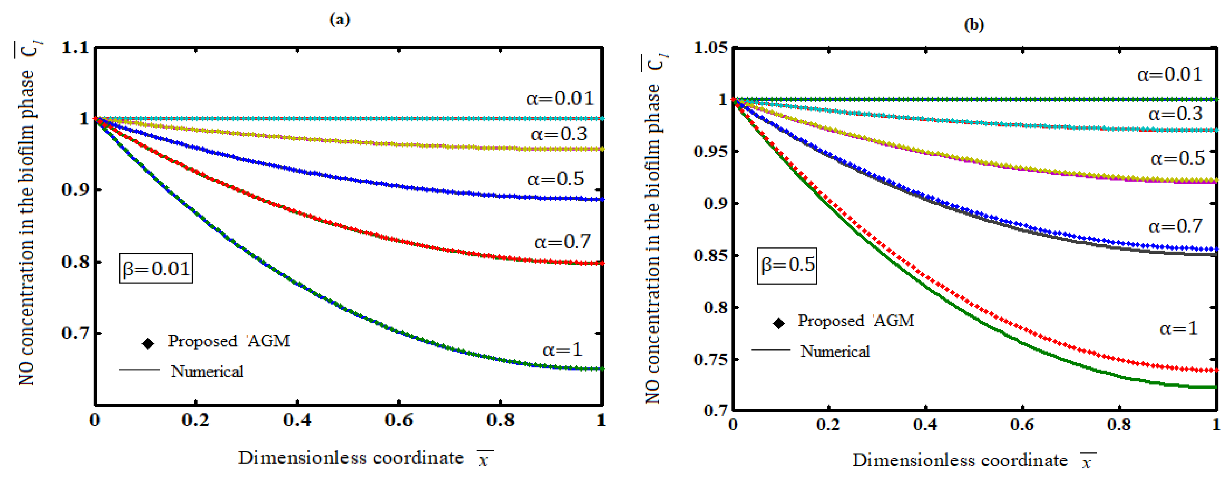
7. Results and Discussion

We note that Equations (15) and (20) defined the AGM-based approximate analytical expressions for the $\mathrm{NO}$ concentration in the biofilm and gas phases, which were valid for all experimental values of the parameters $\alpha , \beta ,\gamma ,\mathrm{and} \eta$. The parameters $\alpha$ and $\eta$ scaled with the biofilm thickness $L_f$. Note that $\beta$ is the inlet $\mathrm{NO}$ concentration. Additionally, we note that $\gamma \left(=\frac{a_f{D}_e}{H U_g}\right)$ was proportional to the specific area of the biofilm $a_f$ and the effective diffusion coefficient $D_e$, and was inversely proportional to the Henry coefficient H and the superficial gas velocity U_g.

The effects that the various parameters $\alpha , \gamma ,\mathrm{and} \eta$ had on the NO concentration profiles are shown in Figure 2a–d. A decrease in all parameters led to a decrease in the concentration of NO in the gas phase $\overline{C_g}$. As the standardized parameter $\beta$ increased, the gas-phase NO concentration $\overline{C_g}$ increased and reached its maximum value when dimensionless height $\overline{z}=0$.

We note that Figure 3a–c represents the concentration profiles of $\mathrm{NO}$ in the biofilm phase $\overline{C_l}$ computed via the AGM-based expression defined in Equation (8) for different values of the parameters, as indicated. From Figure 3a–c, it can be inferred that the concentration of $\mathrm{NO}$ in the biofilm phase $\overline{C_l}$ increases when $\beta$ increases for different values of $\alpha$. The $\mathrm{NO}$ concentration of the biofilm phase reached its maximum when $\alpha <0.01 \mathrm{and} \beta \ge 100$.

Figure 4a–c shows the effect of parameter $\alpha$ on the concentration of NO in the biofilm phase. From the Figures, it was inferred that the concentration of NO decreased when increasing the parameter $\alpha$.

To evaluate the biotrickling filter performance, one should consider the maximum removal efficiency. The reactor design for an industrial application often needs to achieve a high removal percentage. Figure 5 represents the NO removal ratio versus the dimensionless height for various experimental values of the parameters (

Table A2. Experimental Dimensionless Values of the Parameters [13] Used in This Work (Figure 2, Figure 3 and Figure 4 and Table 1).

Dimensionless Parameter	Experimental Value of Parameters Used in [13]	Value of the Parameter Used in Figure 2, Figure 3 and Figure 4 and Table 1	Value of the Parameter Used in Figure 5
$\alpha =L_f\sqrt{\frac{{\mu }_{m X_V}}{Y D_{e }{K}_S}}$	0.1121	0.01 to 20	0.1121
$\beta =\frac{C_g/H}{K_S}$	0.629	0.01 to 500	0.629
$\gamma =\frac{a_f{D}_e}{H U_g}$	0.0126	0.01 to 250	0.0126
$\eta =\frac{{\epsilon }_f{k}_g{C}_{g,0}{L}_f}{U_g}$	10.5	0.01 to 10	10.5

). As indicated in Figure 5, the maximum removal efficiency was reduced accordingly if the inlet concentration was very low. This mathematical procedure can be applied for the removal of volatile organic compounds from air [47,48,49,50,51]. Additionally, this method can be extended for the removal of sulfur dioxide, nitric oxide [52], by the chemical absorption–biological reduction integrated process [6].

Limitation of This Model

Biofilms are formed when microorganisms adhere to surfaces. Because of their function in certain infectious diseases and their importance in many device-related infections, biofilms are extremely important for public health. The term biofilm is sometimes a misnomer, since biofilms are not continuous monolayer surface deposits. Instead, biofilms are highly heterogeneous, containing microcolonies of bacterial cells encased in an EPS matrix and separated from other microcolonies. However, in our model, the assumption about vertical channel, no axial diffusion, and homogeneity in a biofilm are in contrast with the real heterogeneous nature of biofilms.

A fundamental property believed to influence biofilms’ community structures is biofilm thickness. However, since biofilm thickness is inextricably linked to external factors, such as water flow, temperature, development age, and nutrient conditions, its importance is difficult to quantify. Biofilm thickness varies depending on the species, substrate, time required for maturation, and microenvironment conditions, such as nutrient availability and shear flow. Its thickness also depends on the linear velocity $L_f=f\left(t\right)$; the higher the velocity, the thinner the boundary layer. However, in our steady-state model under oligotrophic conditions, we assume that the thickness of the biofilm is constant. This is another limitation of this model.

Biofilms are composed primarily of microbial cells and EPS. EPS can comprise 50% to 90% of the total organic carbon in biofilms and can be considered the primary matrix material of the biofilm. EPS may vary in terms of the nitric oxide diffusion and conversion rates (chemical and physical properties). However, we assumed that the gas phase is moved in a plug flow manner in our model, with no consideration for axial diffusion.

In this paper, a thermophilic biotrickling filter (BTF) system was discussed to inoculate a newly isolated strain of Chelatococcus daeguensis TAD1 for the effective treatment of nitrogen oxide. However, many systems are essentially open, and the observed biofilms always contain a variety of microbial species (e.g., bacteria, fungi, and higher organisms). Our method can also be extended to other microbial species.

8. Conclusions

In this paper, a mathematical model of NOx removal in the gas and biofilm phases of a biotrickling filter is solved to produce an analytical expression for the NO concentration using the Akbari–Ganji method, which has been shown to be effective and reliable. The approximate analytical expression of the NOx concentration in the gas and biofilm phases for all experimental values of the parameters is derived. A satisfactory agreement is noted between the obtained analytical results and the existing numerical results, and indeed with previous approximate solutions. The influence of the biofilm thickness and inflow concentration can be studied using these analytical expressions.

Based on our mathematical expression of the removal efficiency, the optimal parameters of the device could be determined and adjusted in advance to achieve the maximum nitrogen oxide removal efficiency using a biotrickling filter. This type of analysis the biotrickling filter (BTF) model can be used to remove styrene from airstreams, large loads of hydrogen sulphide from biogas streams, and volatile organic compounds from contaminated air.

References

1. Deshusses, M.A.; Shareefdeen, Z. Modeling of Biofilters and Biotrickling Filters for Odor and VOC Control Applications. In Biotechnology for Odor and Air Pollution Control; Shareefdeen, Z., Singh, A., Eds.; Springer: Berlin/Heidelberg, Germany, 2005. [Google Scholar] [CrossRef]
2. Kalantar, M.; Zamir, S.M.; Ferdowsi, M.; Shojaosadati, S.A. Removal of toluene in a biotrickling filter in the presence of methanol vapors: Experimental study, mathematical modeling, and kinetic parameters optimization. J. Environ. Chem. Eng. 2021, 9, 104617. [Google Scholar] [CrossRef]
3. San-Valero, P.; Penya-Roja, J.M.; Alvarez-Hornos, F.J.; Marzal, P.; Gabaldón, C. Dynamic mathematical modelling of the removal of hydrophilic vocs by biotrickling filters. Int. J. Environ. Res. Public Health 2015, 12, 746–766. [Google Scholar] [CrossRef] [PubMed] [Green Version]
4. Apel, W.A.; Turick, C.E. Use of Denitrifying bacteria for the removal of nitrogen oxides from combustion gases. Fuel 1993, 72, 1715–1718. [Google Scholar] [CrossRef]
5. Du Plessis, C.A.; Kinney, K.A.; Schroeder, E.D.; Chang, D.P.Y.; Scow, K.M. Denitrification and nitric oxide reduction in an aerobic toluene-treating biofilter. Biotechnol. Bioeng. 1998, 58, 408–415. [Google Scholar] [CrossRef]
6. Zhao, J.; Xia, Y.; Li, M.; Li, S.; Li, W.; Zhang, S. A biophysicochemical model for no removal by the chemical absorption−biological reduction integrated process. Environ. Sci. Technol. 2016, 50, 8705–8712. [Google Scholar] [CrossRef]
7. Bogner, W.; Krämer, M.; Krutzsch, B.; Pischinger, S.; Voigtländer, D.; Wenninger, G.; Wirbeleit, F.; Brogan, M.S.; Brisley, R.J.; Webster, D.E. Removal of nitrogen oxides from the exhaust of a lean-tune gasoline engine. Appl. Catal. 1995, 7, 153–171. [Google Scholar] [CrossRef]
8. Wang, J.; Wu, C.; Chen, J.; Zhang, H. Denitrification removal of nitric oxide in a rotating drum biofilter. Chem. Eng. J. 2006, 121, 45–49. [Google Scholar] [CrossRef]
9. Chen, J.M.; Ma, J.F. Abiotic and biological mechanisms of nitric oxide removal from waste air in biotrickling filters. J. Air Waste Manag. Assoc. 2006, 56, 32–36. [Google Scholar] [CrossRef] [Green Version]
10. Ramirez, M.; Gómez, J.M.; Aroca, G.; Cantero, D. Removal of hydrogen sulfide by immobilized Thiobacillus thioparus in a biotrickling filter packed with polyurethane foam. Bioresour. Technol. 2009, 100, 4989–4995. [Google Scholar] [CrossRef]
11. Philip, L.; Deshusses, M.A. Sulfur dioxide treatment from flue gases using a biotrickling filter-bioreactor system. Environ. Sci. Technol. 2003, 37, 1978–1982. [Google Scholar] [CrossRef]
12. Jiang, R.; Huang, S.; Chow, A.T.; Yang, J. Nitric oxide removal from flue gas with a biotrickling filter using Pseudomonas putida. J. Hazard. Mater. 2009, 164, 432–441. [Google Scholar] [CrossRef]
13. Liang, W.; Huang, S.; Yang, Y.; Jiang, R. Experimental and modeling study on nitric oxide removal in a biotrickling filter using Chelatococcus daeguensis under thermophilic condition. Bioresour. Technol. 2012, 125, 82–87. [Google Scholar] [CrossRef] [PubMed]
14. Flanagan, W.P.; Apel, W.A.; Barnes, J.M.; Lee, B.D. Development of gas phase bioreactors for the removal of nitrogen oxides from synthetic flue gas streams. Fuel 2002, 81, 1953–1961. [Google Scholar] [CrossRef]
15. Lee, B.D.; Apel, W.A.; Smith, W.A. Oxygen effects on thermophilic microbial populations in biofilter treating nitric oxide containing off-gasstreams. Environ. Prog. 2001, 20, 157–166. [Google Scholar] [CrossRef]
16. Caceres, M.; Silva, J.; Morales, M.; San, R.M.; Aroca, G. Kinetics of the biooxidation of volatile reduced sulphur compounds in a biotrickling filter. Bioresour. Technol. 2012, 118, 243–248. [Google Scholar] [CrossRef]
17. Song, J.; Kinney, K.A. A model to predict long-term performance of vapor phase bioreactors: A cellular automation approach. Environ. Sci. Technol. 2002, 36, 2498–2507. [Google Scholar] [CrossRef]
18. Zarook, S.M.; Shaikh, A.A. Analysis and comparison of biofilter modes. Chem. Eng. J. 1997, 65, 55–61. [Google Scholar] [CrossRef]
19. Meena, V.; Rajendran, L. Analytical expression of concentration profiles of methanol and pinene in air stream and bio-film phase. J. Anal. Bioanal. Tech. 2014, 6, 1–8. [Google Scholar]
20. Meena, V.; Rajendran, L.; Kumar, S.; Jansi Rani, P.G. Mathematical modeling of gas phase and biofilm phase biofilter performance. Egypt J. Basic Appl. Sci. 2016, 3, 94–105. [Google Scholar] [CrossRef] [Green Version]
21. Deshusses, M.A.; Hamer, G.; Dunn, I.J. Behavior of biofilters for waste air biotreatment. 1. Dynamic model development. Environ. Sci. Technol. 1995, 29, 1048–1058. [Google Scholar] [CrossRef]
22. Liao, Q.; Chen, R.; Zhu, X. Theoretical model for removal of volatile organic compound (VOC) air pollutant in trickling biofilter. Sci. China Ser. E 2003, 46, 245–258. [Google Scholar] [CrossRef]
23. Manimegalai, B.; Lyons, M.E.G.; Rajendran, L. A kinetic model for amperometric immobilized enzymes at planar, cylindrical and spherical electrodes: The Akbari-Ganji method. J. Electroanal. Chem. 2021, 880, 114921. [Google Scholar] [CrossRef]
24. Selvi, M.S.M.; Rajendran, L.; Abukhaled, M. Estimation of rolling motion of ship in random beam seas by efficient analytical and numerical approaches. J. Mar. Sci. Appl. 2021, 20, 55–66. [Google Scholar] [CrossRef]
25. Chitra Devi, M.; Pirabaharan, P.; Rajendran, L.; Abukhaled, M. Amperometric biosensors in an uncompetitive inhibition process: A complete theoretical and numerical analysis. React. Kinet. Mech. Catal. 2021, 133, 655–668. [Google Scholar] [CrossRef]
26. Saranya, K.; Mohan, V.; Rajendran, L. Steady state concentrations of carbon dioxide absorbed into phenyl glycidyl ether solutions by residual method. J. Math. Chem. 2020, 58, 1230–1246. [Google Scholar] [CrossRef]
27. Joy Salomi, R.; Vinolyn Sylvia, S.; Rajendran, L.; Abukhaled, M. Electric potential and surface oxygen ion density for planar, spherical and cylindrical metal oxide grains. Sens. Actuators B Chem. 2020, 321, 128576. [Google Scholar] [CrossRef]
28. Joy Salomi, R.; Vinolyn Sylvia, S.; Rajendran, L.; Lyons, M.E.G. Transient current, sensitivity and resistance of biosensors acting in a trigger mode: Theoretical study. J. Electroanal. Chem. 2021, 895, 115421. [Google Scholar] [CrossRef]
29. Manimegalai, B.; Rajendran, L.; Lyons, M.E.G. Theory of the Transient Current Response for the Homogeneous Mediated Enzyme Catalytic Mechanism at the Rotating Disc Electrode. Int. J. Electrochem. Sci. 2021, 16, 210946. [Google Scholar] [CrossRef]
30. Lyons, M.E.G. Understanding the kinetics of catalysed reactions in microheterogeneous thin film electrodes. J. Electroanal. Chem. 2020, 872, 114278. [Google Scholar] [CrossRef]
31. Chitra Devi, M.; Pirabaharan, P.; Lyons, M.E.G.; Rajendran, L. Investigation of the Diffusion Impedance for an Irreversible Redox Reaction. Int. J. Electrochem. Sci. 2021, 16, 210639. [Google Scholar] [CrossRef]
32. Akbari, M.R.; Ganji, D.D.; Nimafar, M.; Ahmadi, R. Significant progress in solution of nonlinear equations at displacement of structure and heat transfer extended surface by new AGM approach. Front. Mech. Eng. 2014, 9, 390–401. [Google Scholar] [CrossRef]
33. Jeyabarathi, P.; Rajendran, L.; Lyons, M.E.G. Reaction-diffusion in a packed-bed reactors: Enzymatic isomerization with Michaelis-Menten Kinetics. J. Electroanal. Chem. 2022, 910, 116184. [Google Scholar] [CrossRef]
34. Akbari, M.R.; Nimafar, M.; Ganji, D.D.; Karimi Chalmiani, H. Investigation on non-linear vibration in arched beam for bridges construction via AGM method. Appl. Math. Comput. 2017, 298, 95–110. [Google Scholar] [CrossRef]
35. Meresht, N.B.; Ganji, D.D. Solving nonlinear differential equation arising in dynamical systems by AGM. Int. J. Appl. Comput. Math. 2017, 3, 1507–1523. [Google Scholar] [CrossRef]
36. Rasi, M.; Kumar, S.; Rajendran, L. Analytical expressions for the concentration of nitric oxide removal in the gas and biofilm phase in a biotrickling filter. J. Assoc. Arab Univ. Basic Appl. Sci. 2015, 18, 19–28. [Google Scholar]
37. Jeyabarathi, P.; Kannan, M.; Rajendran, L. Mathematical Model for Extracting Hollow Fiber Membrane Contactors from Carbon dioxide using Adomian decomposition method. Int. J. Sci. Res. 2020, 9, 6230–6233. [Google Scholar]
38. He, J.H.; El-Dib, Y. Homotopy perturbation method for Fangzhu oscillator. J. Math. Chem. 2020, 58, 2245–2253. [Google Scholar] [CrossRef]
39. He, J.H.; El-Dib, Y. Homotopy perturbation method with three expansions. J. Math. Chem. 2021, 59, 1139–1150. [Google Scholar] [CrossRef]
40. Ali, M.; Anjum, N.; Ain, Q.T.; He, J.H. Homotopy perturbation method for the attachment oscillator arising in nanotechnology. Fibers Polym. 2021, 22, 1601–1606. [Google Scholar] [CrossRef]
41. He, J.H.; El-Dib, Y.O.; Mady, A.A. Homotopy Perturbation Method for the Fractal Toda Oscillator. Fractal Fract. 2021, 5, 93. [Google Scholar] [CrossRef]
42. He, J.H.; Ji, F.Y. Taylor series solution for Lane–Emden equation. J. Math. Chem. 2019, 57, 1932–1934. [Google Scholar] [CrossRef]
43. Jeyabarathi, P.; Rajendran, L.; Abukhaled, M.; Kannan, M. Semi-analytical expressions for the concentrations and effectiveness factor for the three general catalysts shapes. React. Kinet. Mech. Catal. 2022, 1–16. [Google Scholar] [CrossRef]
44. Vinolyn Sylvia, S.; Joy Salomi, R.; Rajendran, L.; Abukhaled, M. Solving nonlinear reaction–diffusion problem in electrostatic interaction with reaction-generated pH change on the kinetics of immobilized enzyme systems using Taylor series method. J. Math. Chem. 2019, 59, 1332–1347. [Google Scholar] [CrossRef]
45. Wazwaz, A.M. Optical bright and dark soliton solutions for coupled nonlinear Schrödinger (CNLS) equations by the variational iteration method. Optik 2020, 207, 164457. [Google Scholar] [CrossRef]
46. Nirmala, K.; Manimegalai, B.; Rajendran, L. Steady-State Substrate and Product Concentrations for Non Michaelis-Menten Kinetics in an Amperometric Biosensor—Hyperbolic Function and Padé Approximants Method. Int. J. Electrochem. Sci. 2020, 15, 5682–5697. [Google Scholar] [CrossRef]
47. Namihira, T.; Tsukamoto, S.; Wang, D.; Katsuki, S.; Hackam, R.; Akiyama, H.; Uchida, Y.; Koike, M. Imrovement of NOX removal efficiency using short-width pulsed power. IEEE Trans. Plasm. Sci. 2000, 28, 434–442. [Google Scholar] [CrossRef]
48. Deshusses, M.A.; Webster, T.S. Construction and economics of a pilot/full-scale biological trickling filter reactor for the removal of volatile organic compounds from polluted air. J. Air Waste Manag. Assoc. 2000, 50, 1947–1956. [Google Scholar] [CrossRef] [Green Version]
49. Hodge, D.S.; Devinny, J.S. Modeling removal of air contaminants by biofiltration. J. Environ. Eng. Sci. 1995, 121, 21–32. [Google Scholar] [CrossRef]
50. Iranpour, R.; Cox, H.H.J.; Deshusses, M.A.; Schroeder, E.D. Literature review of air pollution control biofilters and biotrickling filters for odor and volatile organic compound removal. Environ. Prog. 2005, 24, 254–267. [Google Scholar] [CrossRef]
51. Khan, F.I.; Ghoshal, A.K. Removal of volatile organic compounds from polluted ai. J. Loss Prev. Process. Ind. 2000, 13, 527–545. [Google Scholar] [CrossRef]
52. Han, Y.; Zhang, W.; Xu, J. A simplified mathematical model of multi-species biofilm for simultaneous removal of sulfur dioxide (SO2) and nitric oxide (NO) using a biotrickling-filter. Afr. J. Microbiol. Res. 2011, 5, 541–550. [Google Scholar]
Figure 1. Schematic representation of the NOx concentration distributions in the gas and biofilm phases.
Electrochem 03 00025 g001
Figure 2. Dimensionless NO concentration in the gas phase using Equation (20) for the experimental values (Table A1)of the parameters (a) α . (b) β . (c) η . (d) γ .
Electrochem 03 00025 g002
Figure 3. Dimensionless NO concentration in the biofilm phase C l ¯ computed using Equation (15) for various experimental (Table A2) values of β (when (a) α = 0.01   ( b )   α = 1   ( c )   α = 5 .
Electrochem 03 00025 g003
Figure 4. Dimensionless NO concentration in the biofilm phase C l ¯ computed using Equation (15) for various experimental values of α   and   β   (Table A2) when (a) β = 0.01   ( b )   β = 0.5   ( c )   β = 1 .
Electrochem 03 00025 g004aElectrochem 03 00025 g004b
Figure 5. NOx   removal T ratio NO R for various values of NO i . The experimental values of parameter [8] (Appendix C) are α = 0.1121 ,   β = 0.629 ,   γ = 0.0126 ,   and   η = 10.5 , according to Equation (21).
Electrochem 03 00025 g005