On Computational Asymptotic Analysis of General Sensitive Shells of Revolution


Department of Mathematics and Systems Analysis, Aalto University, FI-00076 Aalto, Finland
Appl. Mech. 2022, 3(3), 1091-1106; https://doi.org/10.3390/applmech3030062
Submission received: 9 July 2022
/
Revised: 15 August 2022
/
Accepted: 22 August 2022
/
Published: 29 August 2022
(This article belongs to the Special Issue Feature Papers in Applied Mechanics)
Abstract
:Recent advances in drug delivery technology have led to renewed interest in shell structures with mixed kinematical constraints, one end clamped, another one free, the so-called sensitive shells. It is known that elliptic sensitive shell problems may not always satisfy the Shapiro–Lopatinsky conditions and hence are not necessarily well-posed. The new observation is that for shells of revolution if the profile function has regions of elliptic Gaussian curvature, that region will dictate the overall response of the structure under concentrated loading. Despite the monotonically increasing total energy as the thickness tends asymptotically to zero, these shells are not in a pure bending state. The numerical results have been verified using equivalent lower-dimensional solutions.
1. Introduction
Thin structures have been studied extensively not only due to their many applications in engineering but also computational challenges related to efficient simulation and analysis of such structures. Shells, in particular, have a wide variety of responses depending on the geometry of the shell, material parameters, boundary conditions, and the types and locations of the forces acting on them, and this list is by no means exhaustive [1]. This means that domain-specific expertise is still required even when modern simulation tools are widely available also for scientists in related fields developing devices with similar structural properties.
This work has been motivated by recent advances in drug delivery technology (see, for instance, the excellent paper by Auvinen et al. [2]). The idea is to construct implantable capsules—possibly patient-specific—that, from an engineering perspective, are, in fact, thin solids of revolution, in other words, monolithic, reservoir-type implants. Auvinen reports on samples with a length of 2 cm and volume of 400 mm3, which are not yet thin due to limitations of the chosen manufacturing process. The payload is an injectable drug-releasing hydrogel formulation. Since the natural objective is to maximise the volume of the payload, the capsules or shells should be as thin as possible. Currently, the state-of-the-art printed nanocellulose sheets have thicknesses in the μm range [3]. There are many strategies for modulating the actual release of the payload; here, the focus is on one where one end of the shell is kinematically constrained (that is, clamped), but the opposite end is free. This class of shell problems is referred to as sensitive shells.
Sensitive shells are not common in engineering since their performance is highly dependent on the geometry of the shell. The book by Sanchez-Palencia [4] is a comprehensive treatise on this topic. The existing theory is limited in the sense that the exact analysis inherently assumes that the variation of the shell profile is uniform in some well-defined way; for instance, the type of the Gaussian curvature does not change. If this assumption does not hold, simulation is the only option available. Each shell is a three-dimensional structure with a thickness d. In analysis and computations, the dimensionless thickness , where L is typically the diameter of the domain, is used instead. This means that the current practical range of dimensionless thicknesses is , where the upper limit is determined by the dimension reduction and thus not by the materials. The solutions to shell problems can often be viewed as linear combinations of local solutions with characteristic length scales that depend on the dimensionless thickness and the local curvature of the shell. Hence it is useful to define the shell surfaces (or parts of them) as either parabolic, hyperbolic, or elliptic.
Sensitivity in thin structures has fascinated many authors. For examples of source problems, see [5,6]. This has also been touched on in the context of eigenproblems, first in [7] and later comprehensively in [8]. Shell structures are also sensitive to imperfections (material or geometric), a problem class which is related yet different from the much narrower range of effects discussed here. For a concise introduction to broader issues related to imperfections, see [9]. In the future, once more experimental data are available, one should consider stochastic analysis where the variation in the curvature is included [10].
The chosen kinematical constraints and loading model require some justification. The clamped end of the shell models the effect of an attached solid, typically a led device used in drug release modulation. The hydrogels are shear thinning and, therefore, it is reasonable not to include fluid–structure interactions into the model. As the drugs are released from the gel, they simply leak out from the open end. When in use, the capsules are subject to external pressure loading, which can be assumed to be uniform under normal circumstances. However, of concern are different impact loads during the use and process of insertion and possibly removal for reuse [11]. The expected drug release rate is based on the ideal shape of the open end of the capsule [2]). Here the focus is on concentrated loads acting on the open end, simulating, for instance, the action of pliers during insertion, as in the classical symmetric pinching problem. This particular loading choice is not restrictive since the action of the concentrated load travels along the characteristics of the surface, and hence qualitatively similar results are obtained even with concentrated loads acting on other parts of the shell [4].
The accurate description of the shell geometry is central since, ultimately, the interesting effects are geometry-dependent. There are many shell models to choose from. In recent years, isogeometric analysis [12] has been promoted as the modern method of choice. From the analysis point-of-view, a much simpler, the so-called mathematical shell model by Pitkäranta [13] is sufficient for the uniform curvature type cases. The model used here is a variant of the Naghdi model [14] for shells of revolution. Using the formulation by Malinen [15], the geometry is also exactly as in the isogeometric case. Sanchez-Palencia’s analysis is based on the Koiter model, which requires finite elements [4].
Any computational study on shells has to account for numerical locking. Within the context of this work, numerical locking is understood as the inevitable loss of the optimal convergence rate [16,17]. No attempts to modify the underlying variational formulation have been made; the loss of the convergence rate is compensated by high-order finite elements, i.e., the hp-version of the FEM [18,19]. A more refined approach for the general case would be to treat the formulation directly [20] or use well-tuned low-order elements [21,22]. Instead of resorting to a fully adaptive solution (see, e.g., [4]), the verification is performed using the symmetry of the problem. The chosen symmetric concentrated load is expanded into a Fourier series in the angular direction, and the corresponding 1D problems are solved with high accuracy. From these 1D solutions, accurate reference values for the quantities of interest can then be derived. The actual 2D computations are calibrated with the 1D reference values, and hence their accuracy can be established with high confidence. This very useful property of the shells of revolution has been used by many authors; see, for instance [7,23].
The main contribution of this study is the observation that the response of any sensitive shell with local elliptic regions will ultimately be dictated by that elliptic region as the dimensionless thickness of the shell tends to zero. Somewhat surprisingly, the angular oscillation typical for purely elliptic sensitive shells emerges in the asymptotic process. This response bears no resemblance to that of the purely parabolic or cylindrical case. This suggests that the insertion procedure has to be carefully designed to account for the sensitivity of the shell structure to minimise possible damage and, thus, indirectly, the performance of the capsule. Another contribution of this paper is to champion the idea of computational asymptotic analysis. Even if the exact mathematical analysis cannot be carried out, through carefully designed numerical experiments, one can derive just as reliable predictive models for decision making.
The rest of this paper is structured as follows: First, the shell problems, including the full exposition of the shell geometries, are introduced. Shell-specific questions of boundary layers and numerical locking are addressed next. Reference results for standard shell profiles are tabulated in Section 4, and the theoretical background for the peculiar behaviour of the purely elliptic sensitive shells under concentrated loading is explained. Finally, numerical experiments on general shell profiles are discussed before the conclusions.
2. Shell Problems
In this section, the shell modelling used throughout this paper is described. Most of this material is standard and has been published in similar formats before but is included for the sake of self-contained presentation. The standard reference is the book by Chapelle and Bathe [1]; of course, Sanchez-Palencia [4] is useful as well.
2.1. Shell Geometry
Thin shells of revolution can formally be characterized as domains in of type
where d is the (constant) thickness of the shell, is a (mid)surface of revolution, and is the unit normal to . The principal curvature coordinates, where there are only four parameters, the radii of principal curvature , , and the so-called Lamé parameters, , , which relate coordinate changes to arc lengths, are needed to specify the curvature and the metric on . The displacement vector field of the midsurface can be interpreted as projections to directions
where is a suitable parametrisation of the surface of revolution, are the unit tangent vectors along the principal curvature lines, and is the unit normal. In other words
In the general case, approximating the principal curvature coordinates is a non-trivial problem.
2.1.1. Profile Functions and Parametrisation
When a plane curve is rotated (in three dimensions) about a line in the plane of the curve, it sweeps out a surface of revolution. Here the two simplest cases are described. Consider a plane curve, the so-called profile function in the -plane, . If the surface is generated by the curve rotating about the x-axis, the profile function and the resulting surface are denoted by and , respectively. If the axis of rotation is the y-axis, and are used instead.
Let be a bounded closed interval, and let be a regular function. The shell midsurface is parameterised by means of the mapping
For , one gets
and
Let be a bounded closed interval with , and let be a regular function. In this case, the shell midsurface is parameterised by means of the mapping
For , one gets
and
Remark 1.
Let us consider the case , , i.e., a parabolic cone. In this case, the directions , coincide for , .
Remark 2.
In the following, without any loss of generality, only examples of are considered.
2.1.2. Classification Based on Gaussian Curvature
The following kinds of shells of revolution, grouped in terms of Gaussian curvature (see, for instance, [24]), cover all fundamental types of midsurface geometry. Refer to Figure 1 for examples. Notice that the classification can also be described in terms of the derivatives of the profile . The analysis of shell problems is greatly simplified if the type of curvature is uniform. In this study, even though this condition does not hold, the classification remains meaningful locally. The three model geometries used in numerical examples are shown in Figure 2.
- 1
- Parabolic (Zero Gaussian curvature shells). One has
- 2
- Elliptic (Positive Gaussian curvature shells). One has
- 3
- Hyperbolic (Negative Gaussian curvature shells). One has
Notice that due to different parametrisations, the profile functions and are not interchangeable in the classifications above.
2.2. Two-Dimensional Model
As mentioned above, the shell model used in the simulations is the so-called Reissner–Naghdi model [14], where the transverse deflections are approximated with low-order polynomials. The resulting vector field has five components , where the first three are the displacements, and the latter two are the rotations in the axial and angular directions, respectively. The convention used is that the computational domain is given by the parametrisation, and the axial/angular coordinates are denoted by x and y. Further, the radii of the principal curvature and the Lamé parameters are assumed to be general.
The total energy is given by a quadratic functional
where represents energy and is the load potential. The constant factor , where E is the Young modulus of the material, and is the Poisson ratio.
Energy is further divided into bending, membrane, and shear energies, denoted by subscripts B, M, and S, respectively.
Bending, membrane, and shear energies are given as
Remark 3.
In the following, we shall omit the constant factor D from the energy expressions. Consequently, all displacements can be considered to be scaled with a factor and energies with a factor .
Using the identities above, the bending, membrane, and shear strains [15], and , respectively, can be written as
Remark 4.
When the shell parametrisations defined above in Section 2.1 are used, all terms of the form are identically zero.
The energy norm is defined in a natural way in terms of the deformation energy (14):
Similarly for bending, membrane, and shear energies:
2.3. Variational Formulation
By minimising the total energy (13) and given an energy space the variational problem becomes: Find such that
and the corresponding finite element problem: Find such that
The load potential has a form
Let us consider a problem where the load acts in the tangential plane of the shell surface, i.e., . It can be shown that if the load holds, problem (30) has a unique weak solution . The corresponding result holds in the finite-dimensional case when the finite element method is employed.
2.4. One-Dimensional Model
The shell model can be further reduced to a one-dimensional one if the load is periodic in the angular direction. This fact is used later in deriving reference solutions for two-dimensional problems. If the load acts in the direction of the u-component, i.e., , , the solution has the form
Using the ansatz above, the energies can be written in terms of the wave number k:
as well as the strains:
The load potential becomes
3. Boundary Layers and Numerical Locking
Shell problems admit a wide variety of boundary layers, including internal ones. In the class of problems considered here, the internal layers play an important role. One of the sources (generators) of layers can be a non-smooth variation of the curvature across some curve on the shell surface. In the numerical experiments below, the profile functions have been chosen so that this effect is not present.
The presence of boundary layers often leads to problems related to numerical locking; that is, the loss of convergence rate due to poor approximation. Using high-order finite element methods is one way to tackle this possible problem [16,17].
3.1. hp-Version of FEM
The finite element method (FEM) is the standard numerical method for solving elliptic partial differential equations. Since FEM is an energy minimisation method, it is eminently suitable for problems in linear elasticity. The hp-FEM variant is the most efficient one [18,19].
The idea behind the p-version is to associate degrees of freedom to topological entities of the mesh in contrast to the classical h-version, where the association is to mesh nodes only. When both strategies are combined, one arrives at the hp-version. The shape functions are based on suitable polynomials, here integrated Legendre polynomials, and their supports reflect the related topological entity, nodes, edges, and the interior of the elements. The nodal shape functions induce a partition of unity. Moreover, due to the construction of shape functions, it is natural to have large elements in the mesh without a significant increase in the discretisation error. Since the number of elements can be kept relatively low given that additional refinement can always be added via the elementwise polynomial degree.
3.2. Layers
The theory of one-dimensional hp-approximation of boundary layers is due to Schwab [19]. Boundary layer functions are of the form
where is a small parameter, is a constant, and L is the characteristic length scale of the problem under consideration. Even though the classical p-method, see, e.g., [18], is capable of asymptotic superexponential convergence, judicious choice of a minimal number of elements using a priori knowledge of the boundary layers leads to a far more efficient solution in the practical range of p.
In the absence of an exact analysis for all of the problem classes discussed below, the central result is given in the form of a definition independent of the dimension of the problem.
Definition 1
(Layer Element Width). For every boundary layer in the problem, optimal convergence can be guaranteed provided there exists an element of width in the direction of the decay of the layer.
Notice that with c constant, if as p increases, the standard p-method can be interpreted as the limiting method.
Boundary layers can also occur within the domains, i.e., be internal layers, or emanate from a point. For the discussion here, it is useful to define the concept of boundary layer generators (see [13]).
Definition 2
(Layer Generator). The subset of the domain from which the boundary layer decays exponentially is called the layer generator. Formally, the layer generator is of measure zero.
The layer generators are independent of the length scale of the problem under consideration.
In Figure 3, the expected layer structures for each of the shell geometries are shown in the case of kinematic constraints and loading considered here. The loading is a symmetric axial pull acting at . Therefore the computational domain can be taken as one-half of the full shell. In parabolic and hyperbolic cases, the singularity is propagated along the characteristics, but since there are no characteristic lines on the elliptic surfaces, the phenomenon is not present. However, there will be trigonometric oscillations along the free boundary with exponentially decaying amplitudes in the axial direction. In all boundaries, in all geometries, there will be parameter-dependent layers as well, but in this setting, they have very low energy content.
3.3. Numerical Locking
One of the challenges in shell problems is to avoid numerical locking. Here, one has to let the higher-order FEM alleviate the locking and accept that some thickness-dependent error amplification or locking factor, , is unavoidable. For the hp-FEM solution, one can derive a simple error formulation
where h is the mesh spacing, L as above, and p is the degree of the elements. It is possible that diverges as t tends to zero, with the worst case being for pure bending problems: . Of course, for , one can expect the hp-solution to be optimal in the sense of approximation theory. This simple error formula also suggests why higher-order methods are advantageous in shell problems: the mesh over-refinement in the “worst” case is , which for a fixed , say, indicates that for the requirement is moderate in comparison to the case of . For a more detailed discussion on this and further references, see [17].
4. Reference Results
In order to fully appreciate the odd world of the sensitive shells, one has to review the reference behaviour in the case of shells with a uniform type of curvature. For the parabolic case, the internal layer has the length scale , whereas for the hyperbolic one the length scale is [13]. For the elliptic case, the oscillations have an angular wave number , in other words, the length scale is only given indirectly [4].
Indeed, the layer structures shown in Figure 3 are clearly identifiable in Figure 4, Figure 5 and Figure 6. Similarly, the parameter dependence of the features is evident. However, what is lost in the scaled colour pictures is that the associated energies in the different cases vary dramatically. The amplitude ranges are given in the respective figure captions.
4.1. Verification Data
Throughout the rest of the paper, the loading is assumed to be symmetric, concentrated pulling in the axial direction; in other words, action on the u-component:
This function can be expanded into a Fourier series in the angular (y) direction, and the reference results can then be calculated as linear combinations of the Fourier weighted 1D solutions. Due to symmetry, only even terms in the cosine series are needed. They can be computed in closed form using special functions and then subsequently evaluated with arbitrary precision. The highest cosine term used in the series is .
The computational domain is with a clamped boundary at , and symmetry conditions at . In one-dimensional simulations, 100 elements at are used, resulting in 2005 degrees of freedom. In 2D simulations, every case is computed on a element grid of quadrilateral elements at (258,405 degrees of freedom). This setup has been calibrated so that the squared energies obtained with 1D and 2D simulations agree over the parameter range (logarithmic subdivision of 41 values). This parameter range is not realistic, as mentioned above. Recall that using modern technologies, in the context of our study, is realistic, as with the traditional engineering setting where is considered the practical range (for instance, car engine parts). However, the selected range is helpful in the verification of theory as well as in the expectation of new materials being introduced. The Poisson number is taken to be . Young’s modulus is effectively , since the results are given without the scaling factor D.
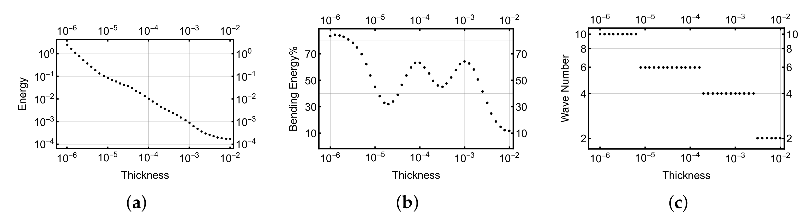
Reference results for the standard cases are tabulated in Table 1. As expected, in the parabolic and hyperbolic cases, the propagation of the singularity does not carry much energy. However, the situation is very different for the elliptic case. In Figure 7, the quantities of interest in the elliptic case are given in terms of graphs. Three observations are imminent, first: the total energy increases as , second: this growth is not simply due to bending, and third: since the loading is symmetric, the oscillations along the free boundary must have even wave numbers, which is the case. Finally, by reading the observed wave numbers, it is clear that the asymptotic rate is indeed the predicted .
4.2. Loss of Coercivity in the Elliptic Case
The reference results in the elliptic case are so different from the others that it is natural to assume that something has failed in the simulations. Surprisingly, the wild behaviour is due to a kind of failure, but not of the simulations, of the model. As in the elliptic case, the model loses coercivity.
More precisely, the Shapiro-Lopatinsky conditions (ellipticity) do not hold on the free boundary; in other words, the problem is not well-posed in the classical sense any more. Sanchez-Palencia devotes an entire chapter to this question ([4], Chapter 8.3.2), where he also mentions that these shells are the only known realistic model where the phenomenon occurs.
5. Numerical Experiments
In the numerical experiments, three different profile functions are examined (see Table 2). The profile functions are selected so that the curvature type does not remain constant, yet each one has a local elliptic region. As for the naming convention, for instance, EH denotes a profile with an elliptic section at the clamped end followed by a hyperbolic section at the free end.
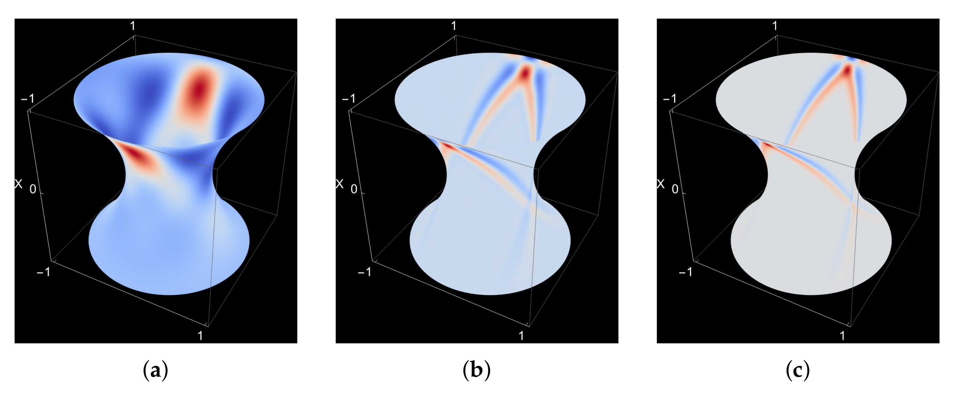
It is rather remarkable that the transverse deflection fields of the different cases are so different in comparison with the reference ones. Even though the concentrated load acts only on a tiny fraction of the boundary, the response of the shell is global in its nature. The singularities are propagated along the characteristics from the parabolic and hyperbolic boundary regions to the elliptic section. The oscillations induced by this excitation, in turn, cause pseudoreflections to return the singularities back to the boundary. Part of the internal layer penetrates into the elliptic section. This is particularly well captured in Figure 8c. One should remember that all cases fall firmly into linear elasticity and hence within the theory of elliptic partial differential equations.
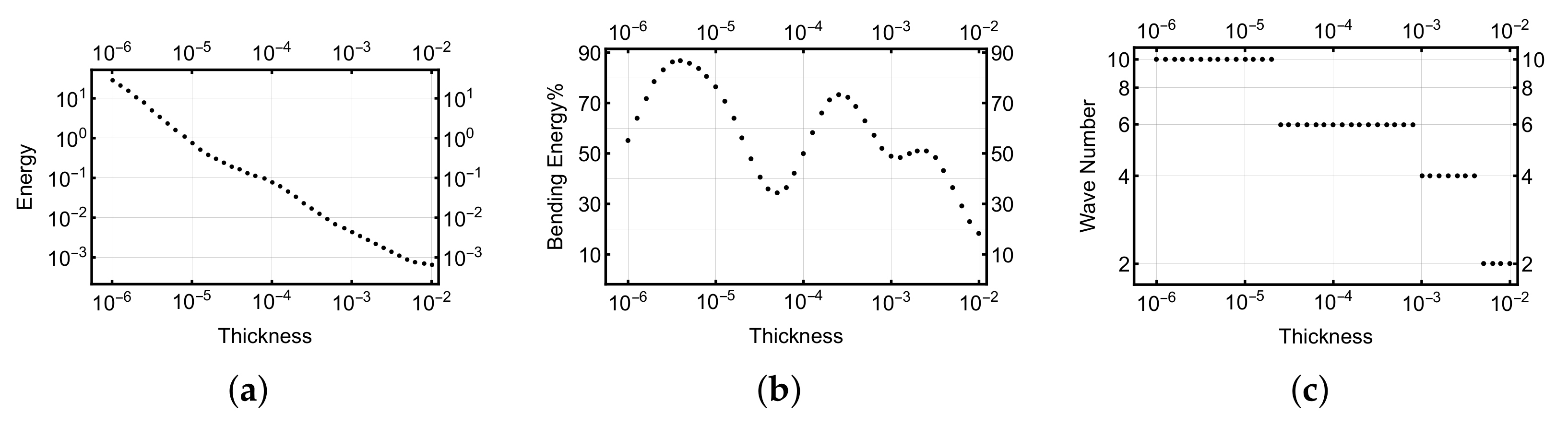
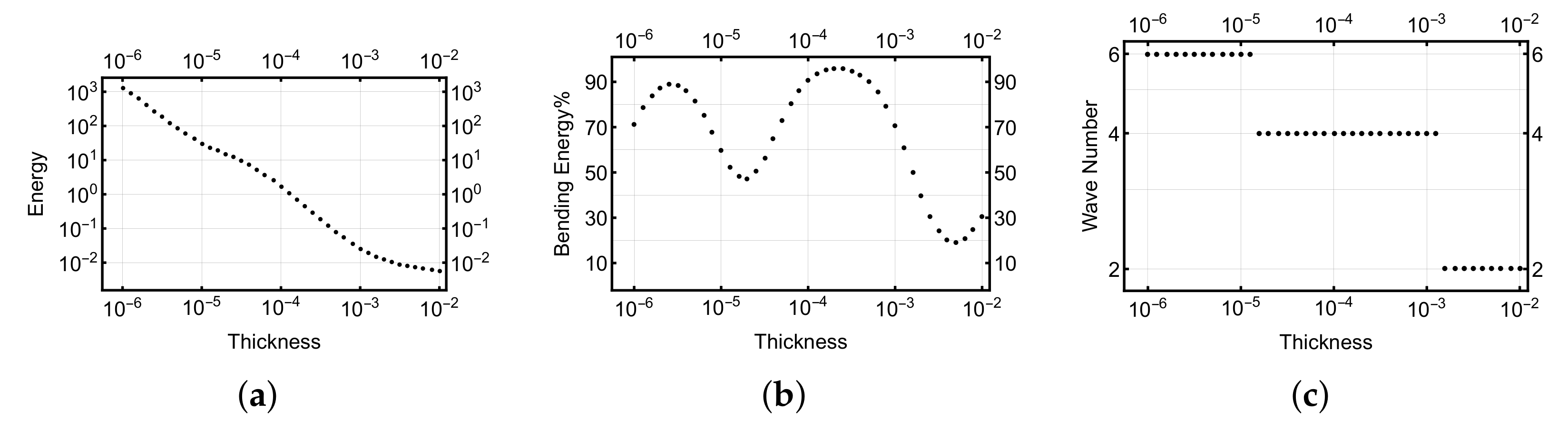
The experiments are summarised in Figure 9, Figure 10, Figure 11, Figure 12 and Figure 13. In terms of energy response, all three cases with general profiles are “elliptic-like.” This is illustrated in Figure 10a, Figure 11a, and Figure 13a. The interpretation is that the elliptic region dictates the overall asymptotic behaviour. This is probably due to the Shapiro-Lopatinsky conditions not being valid in the elliptic region. There are no rigorous theoretical results at the moment supporting this conjecture.
In both Figure 10c and Figure 11c, the observed wave numbers are higher than those of the purely elliptic one. If one compares Figure 8c and Figure 12c, it appears that the hyperbolic region with its two characteristics increases the wave number on the elliptic part, provided that the diameter of the hyperbolic region is sufficiently large. It is possible that this phenomenon is also present in Figure 9c, although it is not in Figure 9b.
Another interesting (and new) observation is the connection between the relative amount of bending energy and the wave number. Instead of being constantly in a pure bending state, the shells transition from one dominant wave number to another via a special state where bending is more restricted. The explanation is not easy to see, however. In fact, there exists a critical thickness at which both oscillations are simultaneously equally strong since the transition must be smooth, and this the only mechanism that can deliver the effect. This is well-known from the theory of free vibration of shells of revolution.
6. Conclusions
New practical applications have brought sensitive shells into focus. The fundamental observation is that for shells of revolution, if the profile function has regions of elliptic Gaussian curvature, then that part is likely to dictate the overall response of the structure under concentrated loading. This is in line with the existing theory on sensitive shells with uniform types of curvature.
The shells of revolution are a useful subset of designs since, through dimension reduction, it is possible to calibrate discretisations via linear combinations of very accurate low-dimensional solutions if, for instance, the loading is such that the Fourier expansion techniques can be applied, as is the case here. Since parameter dependence is always of interest, avoiding more expensive adaptive solutions is advantageous.
In this study, only a very limited set of possible realistic configurations has been addressed. The open-ended capsule designs have to address the specific problems of the sensitivity of the shells. If the chosen design has elliptic regions, the insertion procedure has to be carefully designed to account for the sensitivity of the shell structure to minimise possible damage and, thus, indirectly, the performance of the capsule. In addition, risk assessment for possibilities for impact loading should be performed. Partially constraining the now open boundary would probably lead to yet another class of responses and remains a topic for further study. There are other mechanisms for modulating sustained drug release, for instance, osmotic pumps that fall in the same category depending on the size of the opening. One option is to replace the need for one opening with perforated structures. This is an interesting consideration from the structural point-of-view since the propagation of the singularities within a perforated surface has not received much, if any, attention. Finally, another additional possibility would be to use biodegradable materials, where the structural response would vary over time as the thickness of the shell changes. In any case, the observations reported here remain valid unless the kinematic constraints are strongly altered, for instance, having a perforated structure with closed ends. The drug delivery rate models implicitly assume perfect geometries of the open channels, and any damage or significant change in the profile will affect the predicted performance of the device.
Funding
This research received no external funding.
Data Availability Statement
Not applicable.
Acknowledgments
We acknowledge the computational resources provided by the Aalto Science-IT project.
Conflicts of Interest
The author declares no conflict of interest.
References
- Chapelle, D.; Bathe, K.J. The Finite Element Analysis of Shells; Springer: Berlin/Heidelberg, Germany, 2003. [Google Scholar]
- Auvinen, V.V.; Virtanen, J.; Merivaara, A.; Virtanen, V.; Laurén, P.; Tuukkanen, S.; Laaksonen, T. Modulating sustained drug release from nanocellulose hydrogel by adjusting the inner geometry of implantable capsules. J. Drug Deliv. Sci. Technol. 2020, 57, 101625. [Google Scholar] [CrossRef]
- Yuen, J.D.; Shriver-Lake, L.C.; Walper, S.A.; Zabetakis, D.; Breger, J.C.; Stenger, D.A. Microbial Nanocellulose Printed Circuit Boards for Medical Sensing. Sensors 2020, 20, 2047. [Google Scholar] [CrossRef] [PubMed]
- Sanchez-Palencia, E.; Millet, O.; Béchet, F. Singular Problems in Shell Theory; Springer: Berlin/Heidelberg, Germany, 2010. [Google Scholar]
- Pitkaranta, J.; Sanchez-Palencia, E. On the asymptotic behaviour of sensitive shells with small thickness. Comptes Rendus L’AcadÉMie Des-Sci.-Ser.-Iib-Mech.-Phys.-Chem.-Astron. 1997, 325, 127–134. [Google Scholar] [CrossRef]
- Bathe, K.J.; Chapelle, D.; Lee, P.S. A shell problem ‘highly sensitive’ to thickness changes. Int. J. Numer. Methods Eng. 2003, 57, 1039–1052. [Google Scholar] [CrossRef]
- Artioli, E.; da Veiga, L.B.; Hakula, H.; Lovadina, C. On the asymptotic behaviour of shells of revolution in free vibration. Comput. Mech. 2009, 44, 45–60. [Google Scholar] [CrossRef]
- Chaussade-Beaudouin, M.; Dauge, M.; Faou, E.; Yosibash, Z. High Frequency Oscillations of First Eigenmodes in Axisymmetric Shells as the Thickness Tends to Zero. In Recent Trends in Operator Theory and Partial Differential Equations; Springer International Publishing: Cham, Switzerland, 2017; pp. 89–110. [Google Scholar] [CrossRef]
- Schenk, C.A.; Schuëller, G.I. Uncertainty Assessment of Large Finite Element Systems; Lecture Notes in Applied and Computational Mathematics; Springer: Berlin/Heidelberg, Germany, 2005; Volume 24. [Google Scholar]
- Wang, H.; Guilleminot, J.; Shafer, B.; Tootkaboni, M. Stochastic analysis of geometrically imperfect thin cylindrical shells using topology-aware uncertainty models. Comput. Methods Appl. Mech. Eng. 2022, 393, 114780. [Google Scholar] [CrossRef]
- Laaksonen, T.; (Faculty of Pharmacy, University of Helsinki, Finland). Personal communication, 7 July 2022.
- Benson, D.; Bazilevs, Y.; Hsu, M.; Hughes, T. Isogeometric shell analysis: The Reissner–Mindlin shell. Comput. Methods Appl. Mech. Eng. 2010, 199, 276–289. [Google Scholar] [CrossRef]
- Pitkäranta, J.; Matache, A.M.; Schwab, C. Fourier mode analysis of layers in shallow shell deformations. Comput. Methods Appl. Mech. Eng. 2001, 190, 2943–2975. [Google Scholar] [CrossRef]
- Naghdi, P. Foundations of elastic shell theory. In Progress in Solid Mechanics; North Holland: Amsterdam, The Netherlands, 1963; Volume 4, pp. 1–90. [Google Scholar]
- Malinen, M. On the classical shell model underlying bilinear degenerated shell finite elements: General shell geometry. Int. J. Numer. Methods Eng. 2002, 55, 629–652. [Google Scholar] [CrossRef]
- Pitkäranta, J. The problem of membrane locking in finite element analysis of cylindrical shells. Numer. Math. 1992, 61, 523–542. [Google Scholar] [CrossRef]
- Hakula, H.; Leino, Y.; Pitkäranta, J. Scale resolution, locking, and high-order finite element modelling of shells. Comput. Methods Appl. Mech. Engrg. 1996, 133, 157–182. [Google Scholar] [CrossRef]
- Szabo, B.; Babuska, I. Finite Element Analysis; Wiley: New York, NY, USA, 1991. [Google Scholar]
- Schwab, C. p- and hp-Finite Element Methods; Oxford University Press: Oxford, UK, 1998. [Google Scholar]
- Bieber, S.; Oesterle, B.; Ramm, E.; Bischoff, M. A variational method to avoid locking – independent of the discretization scheme. Numer. Methods Eng. 2018, 114, 801–827. [Google Scholar] [CrossRef]
- Ko, Y.; Lee, P.S.; Bathe, K.J. A new MITC4+ shell element. Comput. Struct. 2017, 182, 404–418. [Google Scholar] [CrossRef]
- Ho-Nguyen-Tan, T.; Kim, H.G. Polygonal shell elements with assumed transverse shear and membrane strains. Comput. Methods Appl. Mech. Eng. 2019, 349, 595–627. [Google Scholar] [CrossRef]
- Hakula, H. hp-boundary layer mesh sequences with applications to shell problems. Comput. Math. Appl. 2014, 67, 899–917. [Google Scholar] [CrossRef]
- Do Carmo, M. Differential Geometry of Curves and Surfaces; Prentice Hall: Upper Saddle River, NJ, USA, 1976. [Google Scholar]
Figure 1.
Shell geometries. (a) Parabolic. (b) Hyperbolic. (c) Elliptic.

Figure 2.
Three examples of shells of revolution with non-uniform type of curvature. (a) Modelname PEHP: . (b) Modelname EH: . (c) Modelname EHEH: .
Figure 2.
Three examples of shells of revolution with non-uniform type of curvature. (a) Modelname PEHP: . (b) Modelname EH: . (c) Modelname EHEH: .

Figure 3.
Boundary layer charts on , where a symmetric concentrated load is acting on point . (a) Parabolic. (b) Hyperbolic. (c) Elliptic (no characteristic curves).
Figure 3.
Boundary layer charts on , where a symmetric concentrated load is acting on point . (a) Parabolic. (b) Hyperbolic. (c) Elliptic (no characteristic curves).

Figure 4.
Parabolic case: transverse deflection profiles. (a) . Range . (b) . Range . (c) . Range .

Figure 5.
Hyperbolic case: transverse deflection profiles. (a) . Range . (b) . Range . (c) . Range .
Figure 5.
Hyperbolic case: transverse deflection profiles. (a) . Range . (b) . Range . (c) . Range .

Figure 6.
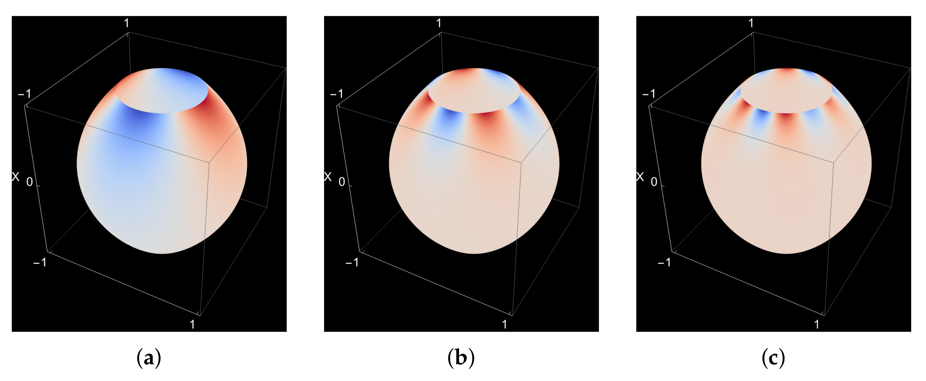
Elliptic case: transverse deflection profiles. (a) . Range . (b) . Range . (c) . Range .

Figure 7.
Elliptic reference case (E). (a) . (b) . (c) Angular wave number.

Figure 8.
Case EH: (a) . Range . (b) . Range . (c) . Range .

Figure 9.
Case PEHP: transverse deflection w profiles. (a) . Range . (b) . Range . (c) . Range .

Figure 10.
Case PEHP: (a) . (b) . (c) Angular wave number.

Figure 11.
Case EH: (a) . (b) . (c) Angular wave number.

Figure 12.
Case EHEH: (a) . Range . (b) . Range . (c) . Range .

Figure 13.
Case EHEH: (a) . (b) . (c) Angular wave number.


Table 1.
Reference energies.
| Case | Profile f(x) = | ||
|---|---|---|---|
| P | 1 | 2 | |
| 4 | |||
| 6 | |||
| H | 2 | ||
| 4 | |||
| 6 | |||
| E | 2 | 0.00484044 | |
| 4 | 35.0395 | ||
| 6 | 546.502 |
Table 2.
Reference data (1D) on experiments.
| Case | Profile | ||
|---|---|---|---|
| PEHP | 2 | 0.000202923 | |
| 4 | 0.0821373 | ||
| 6 | 2.39145 | ||
| EH | 2 | 0.000683408 | |
| 4 | 0.746196 | ||
| 6 | 28.0305 | ||
| EHEH | 2 | 0.00578547 | |
| 4 | 30.9208 | ||
| 6 | 1213.82 |
Publisher’s Note: MDPI stays neutral with regard to jurisdictional claims in published maps and institutional affiliations. |
© 2022 by the author. Licensee MDPI, Basel, Switzerland. This article is an open access article distributed under the terms and conditions of the Creative Commons Attribution (CC BY) license (https://creativecommons.org/licenses/by/4.0/).
Share and Cite
MDPI and ACS Style
Hakula, H. On Computational Asymptotic Analysis of General Sensitive Shells of Revolution. Appl. Mech. 2022, 3, 1091-1106. https://doi.org/10.3390/applmech3030062
AMA Style
Hakula H. On Computational Asymptotic Analysis of General Sensitive Shells of Revolution. Applied Mechanics. 2022; 3(3):1091-1106. https://doi.org/10.3390/applmech3030062
Chicago/Turabian StyleHakula, Harri. 2022. "On Computational Asymptotic Analysis of General Sensitive Shells of Revolution" Applied Mechanics 3, no. 3: 1091-1106. https://doi.org/10.3390/applmech3030062