A New Algorithm to Solve the Extended-Oxley Analytical Model of Orthogonal Metal Cutting in Python

Abstract

This paper presents a new implementation method of the Extended-Oxley analytical model, previously proposed by Lalwani in 2009, for orthogonal cutting of metals with a Johnson–Cook thermo-elastoplastic flow law. The present work aims to improve the implementation of this analytical model in order to propose a unified solution that overcomes the main shortcomings of the original model: the non-uniqueness of the solution, the low accuracy of the obtained solution, and the relatively long computational time for a purely analytical approach. In the proposed implementation, the determination of the optimal set of model parameters is based on an optimization method using the Python LMFIT library with which we have developed a dual Levenberg–Marquardt optimization algorithm. In this paper, the performance and efficiency of the developed model are presented by comparing our results for a 1045 steel with the simulation results obtained in the original paper proposed by Lalwani. The comparison shows a considerable gain in terms of computational speed (more than 2000 times faster than the original model), uniqueness of the obtained solution, and accuracy of the obtained numerical solution (almost zero force imbalance).

1. Introduction

Material removal machining is still one of the most popular manufacturing processes used for the production of mechanical parts in industry today. Depending on the cutting conditions used, and the materials used, the cutting forces and temperatures generated can sometimes be excessive during the chip formation process. These cutting conditions then determine the power requirements of the machine tool and the support load and cause deformations of the workpiece, cutting tools, fixtures, and even the machine tool structure during machining. Understanding what happens during the metal removal process is necessary for the study of the mechanics of machining as well as for tool design and machine tool construction. Several approaches, analytical models, and numerical models are possible, and their choice depends on the needs [1]. Thus, the modeling and simulation of metal machining is an effective means of fine analysis of the cut, but the complexity of the phenomena involved in machining and the lack of knowledge of local mechanisms related to large deformations and high strain rates makes it very difficult to develop these numerical models and costly to use them in terms of time and computing resources. Another way is to globally analyze the cutting process on the basis of an analytical approach; this is much less expensive in terms of numerical resources, but it gives a global result only in terms of cutting forces and temperatures (the local fields given by the numerical simulations are not accessible here).

The present study concerns an innovative implementation of the Extended-Oxley analytical model for metal cutting in Python, using the LMFIT library proposed by Newville et al. [2], to solve the nonlinear equations of the Oxley model and determine the optimal set of internal variables $C_0,\delta ,\varphi$ (defined later) of the Oxley analytical model. Compared to the original models, the approach proposed in this paper allows us to much more efficiently find the solution of the nonlinear system of equations of the Oxley model by allowing a significant gain on the computation time and much higher precision at the level of the equilibrium condition of the efforts of the analytical model.

The structure of this paper consists of a brief synthesis of the orthogonal section and a presentation of the basic equations of the Oxley model (we refer the reader to the numerous publications in the literature for more details concerning the definition of this analytical model). We then present the basics of the Extended-Oxley analytical model proposed by Lalwani [3], then our approach to its numerical implementation in Python with the help of the LMFIT library. A comparison of the results obtained by this approach with those of the literature is then presented in order to validate our resolution method and to evaluate its relative performance. We were able to show a very significant reduction of the computation time, to the order of 2000 times, a very strong improvement of the accuracy of the solution, the uniqueness of the solution, and its independence with respect to the initial conditions. Finally, some global applications of our analytical model are presented to conclude this article.

1.1. Oxley’s Model of Orthogonal Metal Cutting

Since the middle of the twentieth century, many researchers have formulated and improved analytical models of metal cutting using the orthogonal cutting configuration shown in Figure 1, for which the direction of the cutting edge is perpendicular to the plane formed by the cutting velocity (related to the rotation of the workpiece) and the tool feed in a turning configuration.

Merchant [4] developed a planar shear model early on, in the context of orthogonal cut turning, with the assumption that the $\varphi$ shear angle can be determined from minimizing the total power generated by the cutting process. A few years later, Lee and Shaffer proposed a model based on slip line field theory and validated it against experimental results. These early mechanical models of plane shear and slip line did not take into account strain rate effects on the stress values in the machined material. In 1963, Oxley et al. [5] then proposed a slip line model with two distinct shear zones: the primary shear zone (I) in which the material undergoes an abrupt change in flow direction and the secondary shear zone ($II)$ in which friction with the cutting face of the tool generates thermomechanical shear conditions under severe conditions, taking into account the thermomechanical aspect of machining. This model results from the combination of a mechanical part derived from the previous approaches and a thermal part based on the work proposed by Boothroyd [6]. This model takes into account the thermal properties (specific heat $C_p$ and thermal conductivity K of the material to be machined and of the tool) and the effect of stresses, strains, and temperature in the primary shear zone and the tool–chip contact zone. Oxley improved his model over time [5,7], and in 1989 [8], proposed a predictive theory of machining, known as Oxley’s machining theory. This theory predicts, as a function of the cutting conditions (the input parameters of his model, such as speeds, angles, etc.), the cutting forces, the average temperatures, and the stresses and strains in the shear zone and along the tool–chip interface. In his thermomechanical model, and in order to model the flow stress of the material, Oxley uses a power law flow law defined by:

$${\sigma }^y={\sigma }_1{\epsilon }^{p^n},$$

(1)

where ${\sigma }^y$ and ${\epsilon }^p$ are the flow stress and plastic strain, respectively, and the values of ${\sigma }_1$ and n depend on a velocity-modified temperature concept introduced by MacGregor et al. [9].

1.2. The Johnson–Cook Constitutive Flow Law

In order to expand the range of materials that can be used with the Oxley analytical model, Lalwani [3] introduced the Johnson–Cook material flow law [10] into the Oxley analytical model in 2009. This flow law, originally developed to characterize the response of materials subjected to impact loading from explosives, is probably the most widely used for the simulation of high strain rate deformation processes, taking into account the effects of plastic strain, plastic strain rate, and temperature. The following equation gives the general formulation of the yield strength of the material ${\sigma }^y({\epsilon }^p,{\stackrel{.}{\epsilon }}^p,T)$ defined by:

$${\sigma }^y=\left(A+B{\epsilon }^{p^n}\right)\left[1+Cln\left(\frac{{\stackrel{.}{\epsilon }}^p}{{\stackrel{.}{\epsilon }}_0}\right)\right]\left[1-{\left(\frac{T-T_w}{T_m-T_w}\right)}^m\right],$$

(2)

where ${\stackrel{.}{\epsilon }}_0$ is the reference strain rate, $T_w$ and $T_m$ are the initial and the melting temperatures of the material, respectively, and A, B, C, n, and m are the five constitutive flow law parameters. As many efforts have been made in the past to identify the constitutive flow law parameters for many materials, a substantial range of material properties are available in the literature. Conforming to Equation (2), the yield hardening parameter ${\sigma }^h$, defined as the derivative of the yield stress ${\sigma }^y$ with respect to the plastic strain ${\epsilon }^p$, is given by:

$${\sigma }^h=\frac{d{\sigma }^y}{d{\epsilon }^p}={\sigma }^y\frac{nB{\epsilon }^{p^{n-1}}}{A+B{\epsilon }^{p^n}}.$$

(3)

2. The Extended-Oxley’s Model of Orthogonal Metal Cutting

During recent decades, several authors have contributed to the improvement of the cutting model proposed by Oxley in 1989 [8], mainly with the aim of extending its applicability to other materials than those initially used. Thus, Kristyanto [11] extended the range of suitable materials of Oxley’s model to aluminum alloys. Zorev [12] proposed a new model of friction at the tool–workpiece interface that better takes into account the mechanics of contact and the presence of a slippery zone and a sticky zone near the tool tip. Ozel [13], with his PhD thesis, improved the previously proposed models, including the flow stress determination methodology developed by Kumar et al. [14] using the Zorev friction model at the tool–workpiece interface. In order to extend the range of materials for which these analytical cutting models are applicable, and because the parameters of the flow law originally used by Oxley are not available in the literature for a wide range of materials, e.g., for low carbon steel (AISI 1045), Shatla et al. [15], Adibi et al. [16,17], Karpat et al. [18,19], Ozel et al. [20], and Lalwani [3] have replaced the original power form constitutive law, defined by the Equation (1) of the Oxley model, with the Johnson–Cook constitutive law, defined by the Equation (2). Huang et al. [21] subsequently proposed a moving heat source method to model the primary and secondary shear zones and a Johnson–Cook flow law to extend the Oxley model and predict the cutting forces on CBN (Cubic Boron Nitride) tools in hard turning. Chen et al. [22], in contrast, hand used a distributed rectangular heat source near the cutting edge instead of a planar heat source to introduce the temperature generated at the tool–chip interface and also used Johnson–Cook’s flow law to predict the cutting forces for 1045 steel, Al6086-T6, and Ti6Al4V.

In the majority of the papers presenting extensions of Oxley’s original model, the authors have regularly pointed out some shortcomings in Oxley’s original algorithm [5,7,8]. Depending on the implementations and the proposed approaches, they have sometimes found more than one convergent solution when implementing the algorithm or encountered the presence of endless loops or no solution in the recommended search ranges. Some authors have also shown that the prediction accuracy is quite low, and the efficiency of the implemented solution method is very low. Recently, Xiong et al. [23] proposed an original method to replace the three for loops nested in each other, using a combination of constrained optimization function, the genetic algorithm GA, the Patternsearch function, and the multivariate constraints as well as the fmincon optimization algorithm provided by Matlab 2010b to solve this problem. This approach, if it allows for obtaining faster and more accurate results, nevertheless poses the problem of being relatively complex and difficult to implement. The solving methodology proposed in our work is similar to the one proposed by Xiong et al. [23] but differs radically in the numerical means used to solve the system of nonlinear equations. As presented in Section 3, it is relatively simple, close to Oxley’s original algorithm, and can be extended to all the derived forms of Oxley’s original model proposed in the literature insofar as it is external to the equation blocks.

2.1. Brief Recall of the Extended-Oxley’s Model

During the cutting process, as illustrated earlier in Figure 1, and conforming to the mass conservation principle, the produced mass of chip by the unit of time $m_{chip}$ is given by:

$$m_{chip}=\rho V{t}_{1}w,$$

(4)

where $\rho$ is the mass density of the machined specimen, V is the cutting speed, $t_1$ is the depth of cut (related to the advancing speed), and w is the thickness of the workpiece (the width of cut). A two-dimensional illustration of the plastic deformation process involved in an orthogonal machining operation is illustrated in Figure 2, where the main notations related to the proposed analytical cutting model, based on the extension of the Oxley’s theory, are reported.

Oxley’s original analytical model, as well as all the derived models, are based on the need to identify the three internal parameters $C_0,\delta$, and $\varphi$, defining, respectively, the ratio of $l_{AB}$ to the thickness of the primary shear zone (for $C_0$), the ratio of the secondary shear zone thickness to the chip thickness $t_2$ (for $\delta$), and the shear angle (for $\varphi$). Only a precise determination of the values of these three internal parameters allows for obtaining all the results of the model. In the original approach, this triplet of values ensures that the forces in the two shear zones are balanced and that the cutting forces are minimized.

Conforming to Oxley’s analytical model and according to Boothroyd et al. [24], the flow stress is one of the most important equations for both analytical and finite element models. Using the von Mises criterion, and conforming to notations defined in Figure 2, the equivalent shear flow stress $k_{AB}$ in the primary shear zone, along the $AB$ line, can be expressed from the Johnson–Cook flow law given in Equation (2), by the following relationship:

$$k_{AB}=\frac{1}{\sqrt{3}}{\sigma }^y({\epsilon }_{AB}^p,{\stackrel{.}{\epsilon }}_{AB}^p,T_{AB}),$$

(5)

where ${\epsilon }_{AB}^p$, ${\stackrel{.}{\epsilon }}_{AB}^p$, and $T_{AB}$ are the equivalent plastic strain, plastic strain rate, and the average temperature along the $AB$ line, respectively. According to Oxley [8], ${\epsilon }_{AB}^p$ and ${\stackrel{.}{\epsilon }}_{AB}^p$ are considered to be constant, and ${\sigma }_{N_{max}}$, i.e., the maximal value of the normal stress ${\sigma }_N$ at point B (the tool-tip), is given by the following equation:

$${\sigma }_{N_{max}}=k_{AB}\left(1+\frac{\pi }{2}-2\alpha -2C_0{n}_{eq}\right).$$

(6)

where $\alpha$ is the tool rake angle as illustrated in Figure 2, and $n_{eq}$ is the equivalent strain hardening coefficient defined from the constitutive flow law.

Lalwani [3] extended the original Oxley’s model by introducing a modified form of the equation, giving the angle $\theta$, as illustrated in Figure 2, between the resultant of the forces $\overrightarrow{R}$ and the primary shear plane $\left[AB\right]$ with the following expression:

$$tan\theta =1+2\left(\frac{\pi }{4}-\varphi \right)-C_0{n}_{eq},$$

(7)

where, according to the author, the $n_{eq}$ term is defined using the following expression:

$$n_{eq}=\left(\frac{d{\sigma }_{AB}^y}{d{\epsilon }_{AB}^p}\right)\left(\frac{{\epsilon }_{AB}^p}{{\sigma }_{AB}^y}\right),$$

(8)

so that, conforming to the use of the Johnson–Cook flow law given by Equation (2) and its derivative given by Equation (3), the parameter $n_{eq}$ is finally given by:

$$n_{eq}=\frac{nB{\epsilon }_{AB}^{p^n}}{A+B{\epsilon }_{AB}^{p^n}}.$$

(9)

Conforming to Oxley’s theory, the cutting $F_C$ and advancing $F_T$ forces are, respectively, given by:

$$F_C=Rcos\left(\theta -\varphi \right),F_T=Rsin\left(\theta -\varphi \right).$$

(10)

By assuming a uniform normal stress at the tool–chip interface, the normal ${\sigma }_N$ and tangential ${\tau }_{int}$ stresses along the interface are given by:

$${\sigma }_N=\frac{Rcos(\theta +\alpha -\varphi )}{hw},{\tau }_{int}=\frac{Rsin\left(\theta -\varphi \right)}{hw}.$$

(11)

where h is the tool–chip contact length as illustrated in Figure 2. Now comes the most important part of Oxley’s theory. The equilibrium of the internal stresses imposes the following first condition to be ensured, along the primary shear zone, between ${\sigma }_N$ defined by Equation (11) and ${\sigma }_{N_{max}}$ defined by Equation (6):

$${\sigma }_N={\sigma }_{N_{max}}.$$

(12)

In the secondary shear zone, one can compute the flow stress at the tool–chip interface $k_{chip}$ from Equation (2) using:

$$k_{chip}=\frac{1}{\sqrt{3}}{\sigma }^y({\epsilon }_{int}^p,{\stackrel{.}{\epsilon }}_{int}^p,T_{int}).$$

(13)

Equilibrium in the secondary shear zone imposes the following second condition to be ensured between ${\tau }_{int}$ defined by Equation (11) and $k_{chip}$ defined by Equation (13):

$${\tau }_{int}=k_{chip}.$$

(14)

Many more details about these equations and their implementation using the Python language can be found in Dawoua Kaoutoing’s PhD thesis report [25].

2.2. Equilibrium and Nonlinear System to Solve

According to Oxley’s theory, one must satisfy the two equilibrium equations given by Equations (12) and (14) and minimize the cutting force $F_C$ defined by Equation (10). As introduced in the beginning of Section 2.1, in all the previously defined equations, from (6) to (11), there still exist three unknown parameters $\varphi ,C_0$, and $\delta$ to be determined. The final system of nonlinear equations to solve is:

$$\left\{\begin{array}{c}{\sigma }_N(\varphi ,C_0,\delta )={\sigma }_{N_{max}}(\varphi ,C_0,\delta )\hfill \\ {\tau }_{int}(\varphi ,C_0,\delta )=k_{chip}(\varphi ,C_0,\delta )\hfill \\ F_C=min{F}_C(\varphi ,C_0,\delta )\hfill \end{array}\right..$$

(15)

The approach used by Oxley et al. [5,7,8], Lalwani [3], and many other authors for the solution of this system of nonlinear equations consists of determining the set of internal parameters $\varphi ,C_0$ and $\delta$ by introducing a trial and test algorithm based on a triple loop computation, as presented briefly in Figure 3.

As proposed by Oxley, the three parameters are supposed to vary in defined intervals: $\varphi \in [5,45]$, $C_0\in [2,10]$, and $\delta \in [0.005,0.2]$. Oxley thus proposed to set up a resolution algorithm based on three loops nested one in the other ($\varphi$ in $C_0$ and $C_0$ in $\delta$) and to select at each complete iteration the corresponding parameter so that one of the three conditions defined by (15) is satisfied. Thus, $\varphi$ is selected in order to satisfy Equation (14), $C_0$ in order to satisfy Equation (12), and $\delta$ in order to minimize $F_C$ defined by Equation (10). We then easily point out the following main drawbacks of the proposed approach:

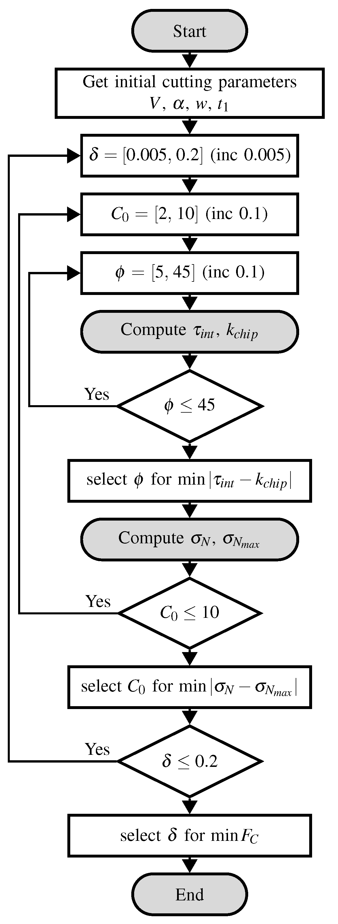
• Because of the range of each of the parameters used and the increment associated with each of them, this leads to 40 values for $\delta$, 81 values for $C_0$, and 401 values for $\varphi$, so that, in order to find the solution, one has to perform a total of $40\times 81\times 401=$ 1,299,240 calculations of ${\tau }_{int}$ and $k_{chip}$ and $81\times 401=$ 32,481 calculations of ${\sigma }_N$ and ${\sigma }_{N_{max}}$, in order to retain at the end only one exploitable result among all these calculations. This approach is far from being an efficient method.
• In contrast, and because of the range of variation of the three parameters, the values selected for the increments of the three parameters are rather coarse, so that the solution is not accurate.
• The algorithm tries to minimize the difference between ${\tau }_{int}(\varphi ,C_0,\delta )$ and $k_{chip}(\varphi ,C_0,\delta )$ at first, then between ${\sigma }_N(\varphi ,C_0,\delta )$ and ${\sigma }_{N_{max}}(\varphi ,C_0,\delta )$, and finally minimizes $F_C(\varphi ,C_0,\delta )$ independently, so that the solution may not be unique, or optimal, at the end, as reported, for example, by Xiong et al. [23].

3. Implementation of the Extended-Oxley’s Model Using Python

In order to solve the system of nonlinear equations shown in Equation (15), we propose here a more efficient approach based on an optimization method implemented in Python language [26]. We have chosen the LMFIT library [2] for the core of the optimization algorithm because it proposes an efficient and easy-to-use implementation of the Levenberg–Marquardt algorithm [27,28].

3.1. Implementation of the Model Using Python

All of the equations presented above defining the Extended-Oxley model were programmed using the Python language, an extended interpreted language with an expressive syntax that some have compared to executable pseudo-code. All development was done using native Python functions, with the only need to import the math module for trigonometric functions. The Python module matplotlib was also used to automatically produce all the graphs presented below. The main function of the program computes the four quantities ${\sigma }_N$, ${\sigma }_{N_{max}}$, ${\tau }_{int}$, and $k_{chip}$ from the three internal parameters $\varphi$, $C_0$, and $\delta$. It also computes, at the same time, all the required results, such as cutting and advancing forces $F_C$ and $F_T$, temperatures $T_{AB}$ and $T_{int}$, and geometric quantities such as h, $l_{AB}$, and $t_2$.

The source files are available on github under a GPL 3.0 license, and the version corresponding to the present publication is available on Zenodo [29].

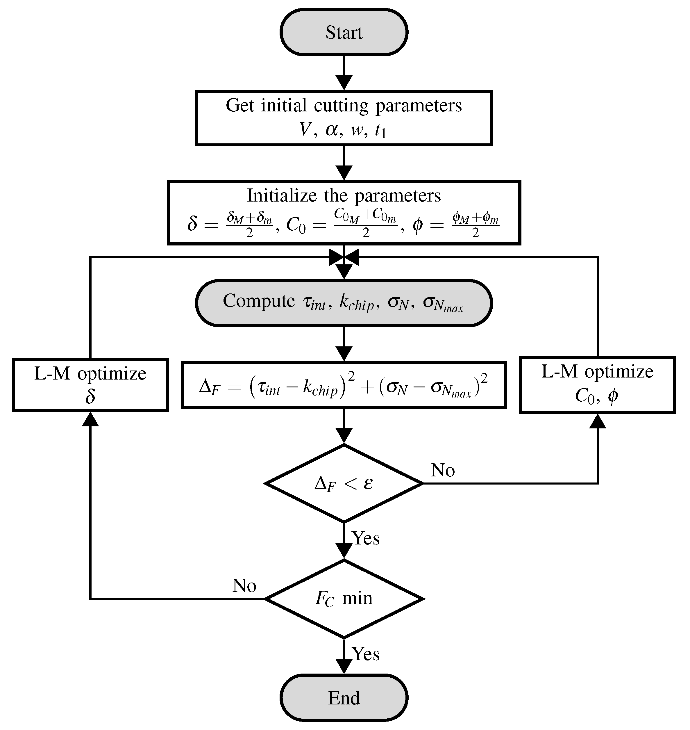
3.2. Solving Algorithm Based on LMFIT

The original part of this work concerns the method used to solve the system of equations defined by (15). Instead of a system similar to the one originally proposed by Oxley [5,7,8] and still used many years later by Lalwani [3], we chose to solve this system using an optimization procedure based on the Python library LMFIT proposed by Newville et al. [2]. The module LMFIT provides a high-level interface for nonlinear optimization and curve fitting problems for Python and provides an access point to the Levenberg–Marquardt algorithm [27,28] of scipy. It can also support most of the optimization methods of scipy.optimize. The main advantage over the standard implementation of scipy is the ability to provide a useful parameter object whose value can vary during fitting, be fixed, or have upper and/or lower bounds. Our program therefore imports the module LMFIT version 1.0.3, which provides the minimization function used to solve the system of equations defined by Equation (15).

Figure 4 presents the general flowchart of the proposed algorithm and shows that two optimization algorithms encapsulated in each other and referred to hereafter as internal optimization algorithm and global optimization algorithm, respectively, are used to obtain the solution of the system in (15). The internal optimization algorithm is in charge of solving the first two equations of the system in (15), corresponding to the Equations (12) and (14), whereas the global optimization algorithm is in charge of finding the minimum value of the cutting force, i.e., the last equation of the system in (15). Thus, due to the interlocking of the two algorithms, the final solution is the one for which the equilibrium condition defined by Equations (12) and (14) is first satisfied by the proposed objective function ${\Delta }_F$, given by the following equation:

$${\Delta }_F=\sqrt{{\left({\tau }_{int}-k_{chip}\right)}^2+{\left({\sigma }_N-{\sigma }_{N_{max}}\right)}^2},$$

(16)

and then the cutting force $F_C$ is minimized in a second step.

In the proposed algorithm, two optimizers objects related to the LMFIT’s minimize function are instantiated at the beginning of the program:

• The first one seeks the optimal value of the parameter $\delta$ ($C_0$ and $\varphi$ are fixed during this optimization step) by minimizing the value of the cutting force $F_C$ defined by Equation (10).
• The second one seeks the optimal value of the parameters $C_0$ and $\varphi$ ($\delta$ is fixed during this optimization step) by minimizing the value of the equilibrium error ${\Delta }_F$ defined by Equation (16). The stop criterion is based on a given precision value $\epsilon$ defined by the user.

In order to know the efficiency of the proposed algorithm, a variable N counts the number of times the central block of instructions used to compute (${\tau }_{int},k_{chip},{\sigma }_N,{\sigma }_{N_{max}}$) is executed. This block of code contains all the CPU intensive computations of our algorithm. The initialization of the three parameters $\varphi ,C_0$, and $\delta$, at the beginning of the computation, is done by arbitrary setting the initial value of each of them to the middle value of their respective intervals. Of course, the independence of the final results with the initial values of the those three parameters was checked, as reported hereafter.

3.3. Validation of the Proposed Algorithm

In order to check how the proposed implementation works, and conforming to the results proposed by Lalwani [3], we present here an example of application concerning the orthogonal cutting of an AISI 1045 steel. Material properties of the AISI 1045 steel are reported in

Table 1. Material properties of the AISI 1045 steel [30].

A (MPa)	B (MPa)	C	n	m
$553.1$	$600.8$	$0.0134$	$0.234$	1
$\stackrel{.}{\mathbf{\epsilon }}{}_{\mathbf{0}}\left(\mathrm{s}{}^{-\mathbf{1}}\right)$	${\mathbf{T}}_{\mathbf{w}}\left(°\mathrm{C}\right)$	${\mathbf{T}}_{\mathbf{m}}\left(°\mathrm{C}\right)$	$\mathbf{\rho }(\mathrm{kg}/{\mathrm{m}}^{\mathbf{3}})$
1	25	1460	8000

.

Thermal conductivity K and heat capacity $C_p$ are dependent of the temperature T through the following equations, respectively:

$$K\left(T\right)=52.61-0.0281T,C_p\left(T\right)=420+0.504T.$$

(17)

The selected cutting conditions for this preliminary test are the following: cutting speed $V=200\mathrm{m}/\min$, depth of cut $t_1=0.15\mathrm{mm}$, tool rake angle $\alpha =-7°$, and width of cut $w=1.6\mathrm{mm}$. All benchmarks tests were solved using Python 3.9.13 on a Dell Precision XPS13 7930 computer running Ubuntu 20.04 64bits with $16\mathrm{GB}$ of RAM and one four-core i7-10510U $1.8\mathrm{GHz}$ Intel Processor. Only one single thread is used for all the simulations; no parallelization of the software has been used for those simulations.

The results of the proposed simulations, in agreement with those proposed by Lalwani [3], are reported in

Table 2. Results for orthogonal machining of AISI 1045 at $V=200\mathrm{m}/\min$, $t_1=0.15\mathrm{mm}$, $\alpha =-7°$, and $w=1.6\mathrm{mm}$.

	${\mathit{C}}_0$	$\mathit{\varphi }(°)$	$\mathit{\delta }$	${\mathbf{\Delta }}_{\mathit{F}}\left(\mathbf{Pa}\right)$
LMFIT	$5.762$	$18.94$	$0.036$	$4.0\times {10}^{-7}$
Lalwani	$5.800$	$18.90$	$0.040$	$4.8\times {10}^6$
gap				$1.2\times {10}^{13}$
	${\mathit{F}}_{\mathit{C}}\left(\mathrm{N}\right)$	${\mathit{F}}_{\mathit{T}}\left(\mathrm{N}\right)$	${\mathit{t}}_{\mathbf{2}}\left(\mathrm{mm}\right)$	$\mathit{h}\left(\mathrm{mm}\right)$
LMFIT	$574.9$	$351.7$	$0.42$	$0.47$
Lalwani	$575.5$	$351.7$	$0.42$	$0.47$
gap	$1.0\times {10}^{-3}$	$0.0$	$0.0$	$0.0$
	${\mathbf{\epsilon }}_{\mathit{AB}}^{\mathit{p}}$	${\mathbf{\epsilon }}_{\mathit{int}}^{\mathit{p}}$	${\mathit{T}}_{\mathit{AB}}\left(°\mathrm{C}\right)$	${\mathit{T}}_{\mathit{int}}\left(°\mathrm{C}\right)$
LMFIT	$0.98$	$11.03$	$356.1$	$954.7$
Lalwani	$0.98$	$10.07$	$356.5$	$945.2$
gap	$0.0$	$8.7\times {10}^{-2}$	$1.1\times {10}^{-3}$	$9.9\times {10}^{-3}$

. The total number of computations of the central block in our algorithm needed to find the final solution is $N=274$. The proposed new algorithm reduces the number of iterations needed to converge to the solution by more than 4700. Concerning the computation time, the algorithm proposed here allows for obtaining the solution in approximately $35\mathrm{ms}$, whereas on the same hardware architecture, the one proposed by Lalwani requires $1\min 16\mathrm{s}$ for the same computation: that is to say an approximate gain of 2150 times faster.

As reported in Table 2, the values of the three internal parameters obtained by the optimization algorithm and the one obtained by the approach used by Lalwani are close, but the number of decimal places is higher in our case, which leads to a finer selection of the optimal solution, explaining the differences found in the results. The total error ${\Delta }_F$ for the equilibrium part of system (15) given by Equation (16) is less than ${10}^{-6}\mathrm{Pa}$. Compared to the results obtained by Lalwani, we note a very large increase in the accuracy of our algorithm. This difference is related to the fact that the three internal variables, due to the presence of loops with fixed increments in the original algorithm, can only vary with a step of $0.1$ for $\varphi$, $0.1$ for $C_0$, and $0.005$ for $\delta$. The optimal solution obtained is still far from the optimum with the original algorithm, as shown by the results reported in Table 2. The cutting and feed forces, as well as the geometry, are close. The results at the primary shear band concerning the deformations ${\epsilon }_{AB}^p$ and temperatures $T_{AB}$ are also very close. However, we note an increase in the plastic deformation ${\epsilon }_{int}^p$ and temperature $T_{int}$ in the case of the approach proposed here, linked in particular to the higher accuracy due to the use of the optimization algorithm. The results remain close, as we only found a gap of the order of ${10}^{-2}$ concerning the evaluation of the temperature $T_{int}$ in the second shear zone.

3.4. The Uniqueness of the Proposed Algorithm

According to Xiong et al. [23], the main drawback of Oxley’s original algorithm and its different variants, such as the one proposed by Lalwani [3], is that the convergent solution is not unique, mainly due to the large errors that can arise from the low precision of the original algorithm (the step length chosen for the parameters is quite coarse, as noted before). A possible alternative is to first search for the minimum point, then to restart a localized search by reducing the domain of variation of the parameters around the last solution and by reducing the search step. The first drawback is that this increases the time needed to find an optimal solution, as it requires several computational steps by reducing the range of variation of the internal parameters at each iteration. The second drawback is to risk finding a local minimum during the first search and then to iterate on this local minimum while remaining unable to converge towards a global minimum.

In order to check if the algorithm proposed here is independent of the starting values, thus not influenced by a possible local minimum in the solution, a total of 15,625 calculations was carried out by varying the starting value of each of the three parameters according to 25 equidistant values in their respective domain of variation. The analysis of these simulations allows knowing whether the final solution obtained is independent of the starting point during the minimization process. The total computational time for these 15,625 simulations is $t=9\min 17\mathrm{s}$, so that the average computational time for a simulation is approximately $t=35\mathrm{ms}$. As shown in

Table 3. Model results for the 15,625 computations.

Parameter	min	max	$\mathbf{\Delta }$
$C_0$	$5.7624545$	$5.7624545$	$1.560\times {10}^{-9}$
$\delta \times {10}^{-2}$	$3.5769311$	$3.5785141$	$4.425\times {10}^{-4}$
$\varphi$	$18.9445809$	$18.9445810$	$5.037\times {10}^{-9}$
$F_C$	$574.9283522$	$574.9283544$	$3.946\times {10}^{-9}$
$F_T$	$351.7365247$	$351.7365280$	$9.439\times {10}^{-9}$
$T_{AB}$	$356.0740228$	$356.0740237$	$2.465\times {10}^{-9}$
$T_{int}$	$954.6387260$	$954.6695481$	$3.229\times {10}^{-5}$

concerning the estimation of the internal parameters, the cutting and advancing forces, and the tool–chip interface temperature, all starting points converge on the same result, i.e., the solution is independent of the initial conditions of the calculation. The only notable difference, very small, concerns the evaluation of the parameter $\delta$ and the temperature of the tool–chip interface $T_{int}$. The error $\Delta$ is computed using the following formula:

$$\Delta =\frac{{\left[\right]}_{max}-{\left[\right]}_{min}}{{\left[\right]}_{mean}},$$

(18)

where ${\left[\right]}_{max}$, ${\left[\right]}_{min}$, and ${\left[\right]}_{mean}$ represent the maximum, minimum, and mean values of the corresponding term over the 15,625 calculations performed for this analysis. Depending on the starting point, the number of loops of the internal optimization algorithm ($C_0$ and $\varphi$) to find the final solution vary in the range $n_{int}\in [194,350]$, with an average value of ${\overline{n}}_{int}=240.6$ and a standard deviation of $\sigma =21.9$, as shown in Figure 5, where the values of the same ten have been grouped together to create the histogram. The number of loops of the global optimization algorithm ($\delta$) vary within the range $n_{ext}\in [18,26]$, with an average value of ${\overline{n}}_{ext}=21.1$ and a standard deviation of $\sigma =2.1$.

3.5. Analysis of the Proposed Algorithm

3.5.1. Selection of the Internal Parameters

Figure 6 shows some essential results concerning the optimization algorithm.

Figure 6a shows the variation of the cutting force $F_C$, the advancing force $F_T$, and the equilibrium error ${\Delta }_F$ vs. $C_0$. The internal parameter $C_0$ has been removed from the optimization procedure and forced to vary within a predefined interval to draw these curves; therefore, only the two remaining internal parameters $\varphi$ and $\delta$ are allowed to be optimized thanks to the LMFIT optimizer. By varying the value of $C_0$ within the range $[2,10]$, we obtained the curves reported in Figure 6a. This graph clearly shows that Equations (12) and (14) cannot be satisfied together as only one parameter (the shear angle $\varphi$) is allowed to vary within the internal optimization procedure; therefore, the equilibrium error ${\Delta }_F$ varies a good deal with the variation of $C_0$: it decreases linearly within the range $C_0\in [2,5.762]$ and increases linearly within the range $C_0\in [5.762,10]$. At the same time, $F_C$ and $F_T$ vary smoothly while increasing within the range $C_0\in [2,9.5]$ and decreases a little after. From this figure, the process for the selection of the solution is clearly illustrated, as we first satisfy the equilibrium defined by Equations (12) and (14) through the satisfaction of the convergence criterion defined by Equation (16). When this one is satisfied, we then select the solution where $F_C$ is minimal. If one had tried to satisfy the condition for $F_C$ being minimal before the equilibrium, the procedure would have selected a lower value for $C_0$, perhaps the value $C_0=2$ (on the left boundary), where obviously the cutting force $F_C$ has a minimum of one.

Figure 6b shows the variation of the cutting force $F_C$, the advancing force $F_T$, and the equilibrium error ${\Delta }_F$ vs. the strain shear angle $\varphi$. On this graph, it can be seen that the cutting forces decreases with the increase in the shear angle $\varphi$, and again the error ${\Delta }_F$ varies a good deal with the value of $\varphi$, with a minimum value, close to zero, at $\varphi =18.945°$.

Figure 6c shows quite a different result. It shows the evolution of the same three results vs. the plastic zone thickness $\delta$. For this case, the equilibrium is always satisfied, as the two parameters $C_0$ and $\varphi$ are involved in the equilibrium, and only the $\delta$ parameter involved in the process of selecting the minimum cutting force is fixed during this analysis. Therefore, the process of selecting the value for $\delta$ that minimizes the force is more or less switched off. Figure 6c shows that the value of the error ${\Delta }_F$ varies when $\delta$ varies within the range $\delta \in [0.005,0.2]$ but always remains less than ${10}^{-6}\mathrm{Pa}$. The process of selecting the final value $\delta =0.036$, which minimizes the cutting force, is clearly illustrated in Figure 6c, as the cutting and advancing forces vary smoothly with the variation of the plastic zone thickness, with a minimum value $\delta =0.036$.

In the end, it is now clear that the full process has selected the set of parameters $\varphi ,C_0,\delta$ so that the equilibrium defined by Equations (12) and (14) is satisfied and the minimal cutting force defined by Equation (10) is obtained. The solution is close to the one obtained by Lalwani [3], but, as there are not any fixed increments for the parameters, the equilibrium error is almost zero in our approach.

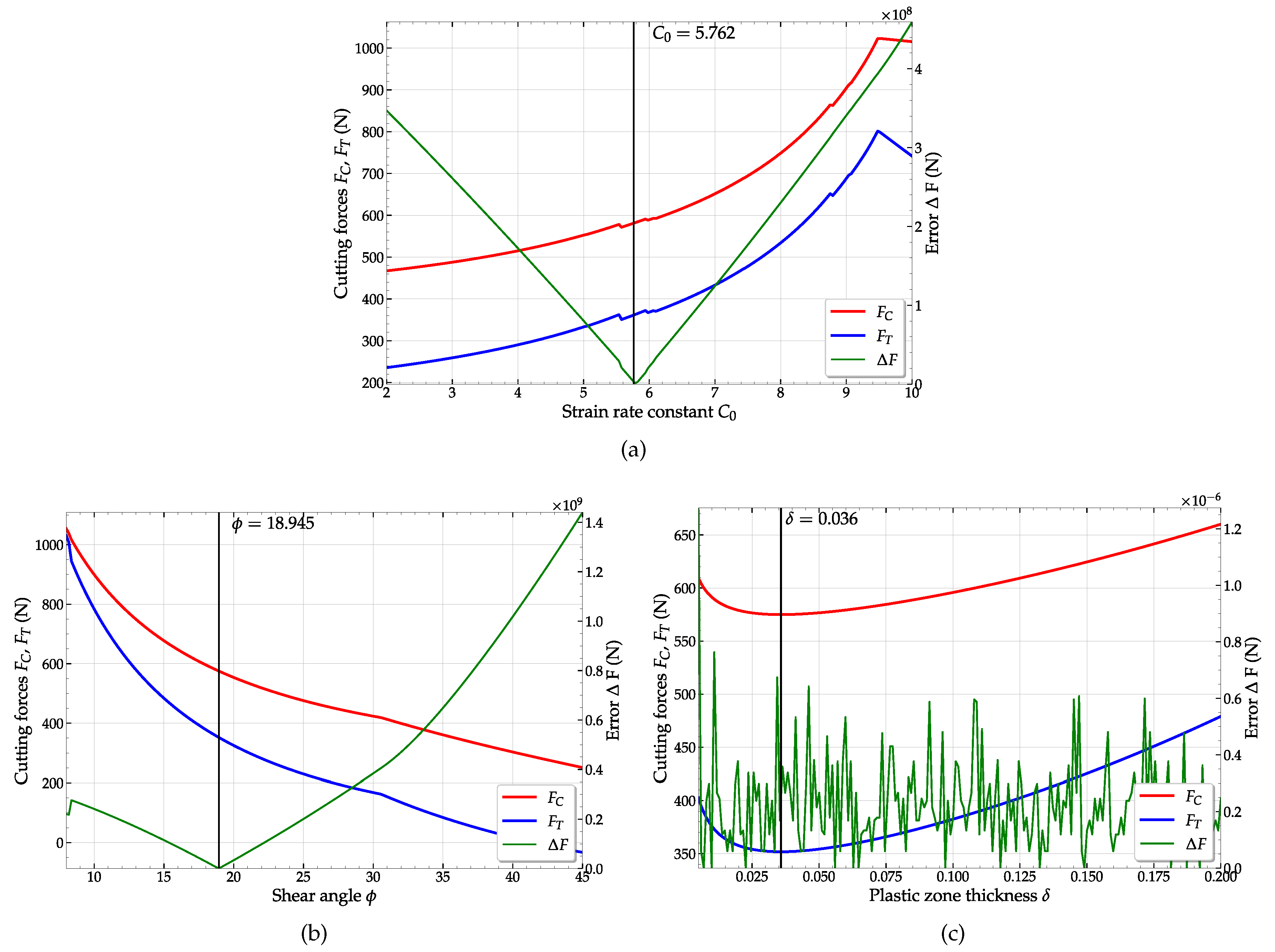
3.5.2. Some Results of the Proposed Algorithm

The proposed algorithm having been validated in the previous section, we now propose to use it to compute results according to any cutting conditions. In order to illustrate this aspect, we have chosen to use the previously used cutting conditions and to study the influence of the cutting speed V and the depth of cut $t_1$ on the numerical results obtained in terms of forces and temperatures. Thus, we selected six different cutting depths $t_1$ in the range $[0.15,0.5]\mathrm{mm}$ and a cutting speed V varying from $100\mathrm{m}/\min$ to $400\mathrm{m}/\min$. Figure 7a shows the variation of interface temperature $T_{int}$ as a function of cutting speed V for the six values of cutting depth $t_1$.

As shown in this figure, $T_{int}$ increases smoothly with increasing cutting speed V until it reaches the melting temperature $T_m$ and also increases with increasing cutting depth $t_1$. Therefore, it is not possible, for example, to obtain a solution for the depth of cut $t_1\ge 0.25\mathrm{mm}$ over the entire range of cutting speed $[10,400]\mathrm{m}/\min$ but only over a reduced range (e.g., only over $V\in [100,175]\mathrm{m}/\min$ for $t_1=0.5\mathrm{m}/\min$). Figure 7b,c show the variation of cutting force $F_C$ and advancing force $F_T$ as a function of cutting speed V and cutting depth $t_1$. As shown in these two figures, both forces decrease with increasing cutting speed V, mainly due to the softening of the material because of the high dependence of the temperature generated during cutting on the cutting speed, as shown in Figure 7a.

4. Conclusions

A new algorithm for solving the Extended-Oxley analytical model for orthogonal cutting of metals and its implementation using the LMFIT library in Python were proposed [29]. Compared to the original implementation proposed by Lalwani [3], the performance in terms of computational speed and improvement of computational accuracy is considerable (a gain in computational time having a factor of approximately x1900 and almost zero error regarding the imbalance of internal forces). The predicted values of the cutting force $F_C$, the advancing force $F_T$, and the temperatures $T_{AB},T_{int}$ are computed with a total error of the equilibrium part of the system of less than ${10}^{-6}\mathrm{Pa}$ for our approach, whereas the same error is approximately $20\mathrm{MPa}$ for the original algorithm. The uniqueness of the solution when using this new solving algorithm, which addresses one of the major drawbacks of the original approach as noted in the literature, has been demonstrated and validated in this paper. The proposed approach, based on two Levenberg–Marquardt optimization algorithms for solving the system of nonlinear equations of Oxley’s analytical cutting model, has been shown to be effective, accurate, and efficient in terms of computational time during validation tests. The speed of this new algorithm, as well as the improvement of the accuracy and stability of the solution, allows us to consider its use in a real-time machining monitoring system. We can thus consider the integration of this model in a supervision device that controls in real-time according to the cutting conditions, such that the machining forces remain in an acceptable range and allows for the detection of a failure of the cutting tool in real time.

References

1. Sousa, V.; Silva, F.J.G.; Fecheira, J.S.; Lopes, H.M.; Martinho, R.P.; Casais, R.B. Accessing the cutting forces in machining processes: An overview. Procedia Manuf. 2020, 51, 787–794. [Google Scholar] [CrossRef]
2. Newville, M.; Stensitzki, T.; Allen, D.B.; Rawlik, M.; Ingargiola, A.; Nelson, A. LMFIT: Non-Linear Least-Square Minimization and Curve-Fitting for Python. 2021. Available online: https://ui.adsabs.harvard.edu/abs/2016ascl.soft06014N/abstract (accessed on 23 June 2022).
3. Lalwani, D. Extension of Oxley’s predictive machining theory for Johnson and Cook flow stress model. J. Mater. Process. Technol. 2009, 209, 5305–5312. [Google Scholar] [CrossRef]
4. Merchant, M. Mechanics of the metal cutting process I. Orthogonal cutting and a type 2 chip. J. Appl. Phys. 1945, 16, 267–275. [Google Scholar] [CrossRef]
5. Oxley, P.; Welsh, M. Calculating the shear angle in orthogonal metal cutting from fundamental stress-strain-strain rate properties of the work material. In 4th International Machine Tool Design and Research Conference, The College of Aeronautics Cranfield; Pergamon Press: Oxford, UK, 1964. [Google Scholar]
6. Boothroyd. Temperatures in orthogonal metal cutting. Proc. Inst. Mech. Eng. 1963, 177, 789–802. [Google Scholar] [CrossRef]
7. Oxley, P.; Hastings, W. Minimum work as a possible criterion for determining the frictional conditions at the tool/chip interface in machining. Philos. Trans. R. Soc. London. Ser. A Math. Phys. Sci. 1976, 282, 565–584. [Google Scholar] [CrossRef]
8. Oxley, P.L.B. Mechanic of Machining: An Analytical Approach to Assessing Machinability; Ellis Horwood Limited: Chichester, UK; John Wiley and Sons: New York, NY, USA, 1989. [Google Scholar] [CrossRef] [Green Version]
9. MacGregor, C.; Fisher, J. A velocity-modified temperature for the plastic flow of metals. J. Appl. Mech.-Trans. ASME 1946, 13, A11–A16. [Google Scholar] [CrossRef]
10. Johnson, G.; Cook, W. A constitutive model and data for metals subjected to large strains, high strain rates and high temperatures. In Proceedings of the 7th International Symposium on Ballistics, The Hague, The Netherlands, 19–21 April 1983; Volume 21, pp. 541–547. [Google Scholar]
11. Kristyanto, B.; Mathew, P.; Arsecularatne, J. Determination of Material Properties of Aluminum From Machining Tests. In Proceedings of the ICME 2000-Eighth International Conference on Manufacturing Engineering, Sydney, Australia, 27–30 August 2000; pp. 27–30. [Google Scholar]
12. Zorev, N. Interrelationship between the shear processes occurring along the tool face and on the shear plane in metal cutting. In International Research in Production Engineering; American Society of Mechanical Engineers: New York, NY, USA, 1963; pp. 143–152. [Google Scholar]
13. Ozel, T. Investigation of High Speed Flat End Milling Process-Prediction of Chip Formation, Cutting Forces, Tool Stresses and Temperatures. Ph.D. Thesis, The Ohio State University, Columbus, OH, USA, 1999. [Google Scholar]
14. Kumar, S.; Fallboehmer, P.; Altan, T. Computer Simulation of Orthogonal Metal Cutting Process: Determination of Material Properties and Effects of Tool Geometry on Chip Flow. Trans.-N. Am. Manuf. Res. Inst. SME 1997, 33–38. [Google Scholar]
15. Shatla, M.; Kerk, C.; Altan, T. Process modeling in machining. Part I: Determination of flow stress data. Int. J. Mach. Tools Manuf. 2001, 41, 1511–1534. [Google Scholar] [CrossRef]
16. Adibi-Sedeh, A.; Madhavan, V. Effect of some modifications to Oxley’s machining theory and the applicability of different material models. Mach. Sci. Technol. 2002, 6, 379–395. [Google Scholar] [CrossRef]
17. Adibi-Sedeh, A.; Madhavan, V.; Bahr, B. Extension of Oxley’s analysis of machining to use different material models. J. Manuf. Sci. Eng. 2003, 125, 656–666. [Google Scholar] [CrossRef] [Green Version]
18. Karpat, Y.; Özel, T. Predictive analytical and thermal modeling of orthogonal cutting process-part I: Predictions of tool forces, stresses, and temperature distributions. J. Manuf. Sci. Eng. 2006, 128, 435–444. [Google Scholar] [CrossRef]
19. Karpat, Y.; Özel, T. Predictive analytical and thermal modeling of orthogonal cutting process-part II: Effect of tool flank wear on tool forces, stresses, and temperature distributions. J. Manuf. Sci. Eng. 2006, 128, 445–453. [Google Scholar] [CrossRef]
20. Ozel, T.; Zeren, E. A methodology to determine work material flow stress and tool-chip interfacial friction properties by using analysis of machining. J. Manuf. Sci. Eng. 2006, 128, 119–129. [Google Scholar] [CrossRef]
21. Huang, Y.; Liang, S. Cutting forces modeling considering the effect of tool thermal property—application to CBN hard turning. Int. J. Mach. Tools Manuf. 2003, 43, 307–315. [Google Scholar] [CrossRef]
22. Chen, Y.; Li, H.; Wang, J. Further development of Oxley’s predictive force model for orthogonal cutting. Mach. Sci. Technol. 2015, 19, 86–111. [Google Scholar] [CrossRef]
23. Xiong, L.; Wang, J.; Gan, Y.; Li, B.; Fang, N. Improvement of algorithm and prediction precision of an extended Oxley’s theoretical model. Int. J. Adv. Manuf. Technol. 2015, 77, 1–13. [Google Scholar] [CrossRef]
24. Knight, W.A.; Boothroyd, G. Fundamentals of Metal Machining and Machine Tools; CRC Press: Boca Raton, FL, USA, 2005; Volume 198. [Google Scholar] [CrossRef]
25. Kaoutoing, M.D. Contributions à la Modélisation et la Simulation de la Coupe des Métaux: Vers un Outil d’aide à la Surveillance par Apprentissage. Ph.D. Thesis, Génie Mécanique, Mécanique des Matériaux, INPT, Toulouse, France, 2020. [Google Scholar]
26. Rossum, G. Python Reference Manual; Technical Report; Stichting Mathematisch Centrum: Amsterdam, The Netherlands, 1995. [Google Scholar]
27. Levenberg, K. A method for the solution of certain non-linear problems in least squares. Q. Appl. Math. 1944, 2, 164–168. [Google Scholar] [CrossRef] [Green Version]
28. Marquardt, D. An algorithm for least-squares estimation of nonlinear parameters. J. Soc. Ind. Appl. Math. 1963, 11, 431–441. [Google Scholar] [CrossRef]
29. Pantalé, O. The ExtOxley-LMFIT Software; Zenodo. 2022. Available online: https://zenodo.org/record/6698434#.Ys-bD2BBxPY (accessed on 23 June 2022).
30. Jaspers, S.P.F.C.; Dautzenberg, J.H. Material behaviour in conditions similar to metal cutting: Flow stress in the primary shear zone. J. Mater. Process. Technol. 2002, 122, 322–330. [Google Scholar] [CrossRef]
Figure 1. Orthogonal metal cutting configuration.
Applmech 03 00051 g001
Figure 2. Chip formation conforming to Oxley’s model.
Applmech 03 00051 g002
Figure 3. The simplified flowchart implementation for the computation of ϕ , C 0 , δ conforming to the one proposed by Oxley [8].
Applmech 03 00051 g003
Figure 4. General flowchart of the proposed Oxley–LMFIT model.
Applmech 03 00051 g004
Figure 5. Histogram of the total number of loops to get a solution.
Applmech 03 00051 g005
Figure 6. Cutting forces F C , F T and equilibrium error Δ F evolution vs. strain rate constant C 0 (a), vs. shear angle ϕ (b), and vs. plastic zone thickness δ (c).
Applmech 03 00051 g006
Figure 7. Interface temperature T i n t (a), cutting force F C (b), and advancing force F T (c) evolution vs. cutting speed V and depth of cut t 1 .
Applmech 03 00051 g007