Article

An Inverse Identification Procedure for the Evaluation of Equivalent Loading Conditions for Simplified Numerical Models in Abaqus

Laboratoire Génie de Production, Institut National Polytechnique/Ecole Nationale d’Ingénieurs de Tarbes, Université de Toulouse, 47 Av d’Azereix, F-65016 Tarbes, France
*
Author to whom correspondence should be addressed.
These authors contributed equally to this work.
Appl. Mech. 2022, 3(2), 663-682; https://doi.org/10.3390/applmech3020039
Submission received: 19 April 2022 / Revised: 10 June 2022 / Accepted: 15 June 2022 / Published: 17 June 2022
(This article belongs to the Special Issue Impact Mechanics of Materials and Structures)

Abstract

:
In the finite element simulation process, it is very common to use simplified models to replace the original complex models to reduce the computational cost. To improve the accuracy of simulation with simplified numerical models in Abaqus Explicit, we propose an inverse identification procedure to evaluate the equivalent loading conditions to be applied to these simplified models. We construct an objective function to test the correlation between the final deformed shape obtained by simulation on the full models and the simplified models. A Python identification program using the Levenberg–Marquardt algorithm is implemented to optimize this objective function. In parallel to this approach, we propose a data processing step, validated by a dynamic tensile test, to obtain more accurate numerical responses, including data extraction and estimation. Full numerical models for the Taylor test, dynamic tensile test, and dynamic shear test were constructed using Abaqus Explicit FEM code. The complete models were then replaced by simplified models, in which some non-essential parts were removed and some boundary conditions were modified. In order to obtain the same results in terms of the final geometry, the proposed inverse identification procedure is then used to calculate the equivalent impact velocities for the simplified models.

1. Introduction

In dynamic mechanics, we can distinguish two problems: the direct problem and the inverse problem [1]. We can define the direct problem as the search for the solution of a system of equations according to given boundary conditions and inputs. Concerning the inverse problem, we can divide it into two categories, namely the classical identification problem and the inverse identification problem.
  • The classical identification problem consists of finding the model describing the system from given inputs, responses, and boundary conditions.
  • The inverse identification problem consists of finding the inputs of the system, based on the given responses, boundary conditions and model of the system (the main concern of this work).
The inverse identification method has been studied and developed over the past few decades. The basic principle of this method is the comparison between experimental measurements and numerical results calculated by the finite element method. A common application of this method is the identification of unknown parameters for constitutive laws [2,3,4]. The unknown material parameters in the numerical model are adjusted iteratively to match experimental measurements and numerical calculation results as closely as possible for the same experimental procedure.
In finite element simulation, it is very common to use simplified models to replace the original complex models in order to reduce the computational cost. For example, 2D models are widely used to replace 3D models, some non-essential parts of numerical models are removed, some complex boundary conditions are replaced by simpler ones, etc. These simplifications improving the computational efficiency can be a source of errors if we simulate the simplified models under the same loading conditions as the original models (such as applied loading, temperature, impact velocity, etc.). Thus, the determination of equivalent loading conditions becomes necessary for the simplified models in order to improve the accuracy of the numerical simulation.
In this paper, an inverse identification procedure is used for the evaluation of equivalent loading conditions for simplified numerical models in the Abaqus Explicit finite element code. This procedure is no longer concerned with the comparison between experimental and numerical responses, but with the comparison between the numerical responses of the full models and the numerical responses of the simplified models. In the Section 2, a Python identification program using the Levenberg–Marquardt algorithm is implemented to optimize the objective function. A data processing step, presented in Section 3, is proposed to obtain more accurate numerical answers, including extraction and estimation of dimensional measures. In Section 4, the effectiveness of the proposed identification procedure is validated by three examples, which consist of identifying the equivalent impact velocities for the simplified models of the Taylor test, the dynamic tensile test, and the dynamic shear test.

2. The Identification Program

In the past, the technique of parameter identification was usually the sequence of rather tedious manual processes. Nowadays, the advancement of computer hardware allows an approach where an optimization method, usually based on the use of the least squares method, is most often used to find the required set of parameters. In this approach, the residual between the measured data and the calculated model response becomes the objective function to be minimized [5].
The inverse identification method has already been developed and used in the LGP laboratory (Laboratoire Génie de Production) [3,6,7,8,9]. In his PhD thesis work, I. Nistor proposed a complete identification procedure in which the difference between the numerically deformed shape and the experimentally deformed shape was minimized by a combined Monte–Carlo and Levenberg–Marquardt algorithm. In his work, the Johnson–Cook constitutive law parameters for 42CrMo4 steel and 2017-T3 aluminum were identified using Taylor impact tests. Subsequently, two new dynamic tests using the same Taylor gas gun setup for the identification of the high-velocity friction law [6] and the identification of a dynamic crack propagation criterion [7] were developed. Based on the same identification algorithm, the same research team later proposed a new tensile test [10] used for the identification of metallic material behaviors using the Taylor impact technique.
In the present work, a new identification program is developed to calculate the correlation between the final deformed shape of the full numerical models and the final deformed shape of the simplified numerical models using the Python language (the previous version was implemented in C++). In this new version of the identification program, we have made many improvements to increase the robustness and stability of the identification procedure.

2.1. Objective Function

In the identification procedure, we must first construct an objective function that takes the values of the final deformed shape of the full models and the final deformed shape of a simplified model and computes the residuals to be minimized. Although the optimization methods chosen for minimization are diverse, the mathematical formulations of the objective functions in almost all papers are expressed using a norm [3,11,12]. The general form can be improved by taking into account weights on the results, the type of norm, or by introducing uncertainties on the numerical results. In this case, the objective function f o is expressed by a Euclidean norm form, with the following expression:
f o = 1 m j = 1 m w r j r s j r c j r c j 2
where m is the total number of responses, w r is the vector of response weights, r s is the vector of numerical responses of the simplified model, and r c is the vector of numerical responses of the full model. The term r s j r c j r c j must make the residuals dimensionless. Moreover, r s is a function of the loading conditions, defined by:
r s = r s ( c 1 , c 2 , . . . )
where c 1 , c 2 , are the parameters of the loading conditions. Usually, different loading conditions lead to different numerical responses. The goal of the identification program is to search for appropriate loading conditions that minimize the value of the objective function f o using gradient methods.

2.2. The Levenberg–Marquardt Algorithm and the Lmfit Python Library

2.2.1. The Levenberg–Marquardt Algorithm

The Levenberg–Marquardt (LM) algorithm is a widely adopted iterative technique for locating the minimum of a multivariate function expressed as the sum of squares of real–valued non–linear functions [13,14,15]. It has become a standard technique for nonlinear least squares problems. The principle of using the LM algorithm to minimize the proposed objective function is the uniqueness of the minimum, otherwise we could obtain a local minimum and not a global minimum by the LM algorithm. It could be shown from the previous experiment that the minimum of the above proposed objective function is unique (there are no local minima in the standard parameter variation spaces). Therefore, in the new identification program, only the LM algorithm is used to perform the minimization (we no longer use the combination with the Monte–Carlo algorithm). We can consider the LM method as a combination of the steepest descent method and the Gauss–Newton method.

2.2.2. The Lmfit Python Library

To perform the objective function optimization using the Levenberg–Marquardt algorithm, the Python language library lmfit [16] is used. It was designed to provide simple tools for building complex fitting models for nonlinear least squares problems and applying these models to real data. It builds on and extends many of the optimization algorithms in the Python module scipy.optimize, including the Levenberg–Marquardt method of the optimize.leastsq algorithm. Although the minimization process can be performed with the Python module scipy.optimize, there are several practical pitfalls, including:
  • Although there is no intrinsic meaning, we must keep track of the order and meaning of the variables.
  • If we change the variation of a variable, the objective function must be modified, which is a heavy work for more complex models.
  • Variable boundaries or mathematical relationships between variables are difficult to enforce.
The lmfit module fills these gaps by using objects—an essential reason for working with Python. The key concept of the lmfit module is to replace ordinary floating-point numbers with Parameter objects as the variables of the fit. Using these Parameter objects (or the closely related Parameters module—a dictionary of Parameter objects), we can:
  • Refer to variables directly by name without worrying about their order and meaning.
  • Easily define limits as attributes of variables.
  • Change the variation of variables without having to rewrite the objective function.
  • Place algebraic constraints on variables.
The function minimize embedded in lmfit is used to run an optimization problem. It takes an objective function, an object Parameters, and several optional arguments controlling the convergence of the minimization algorithm to perform an adjustment of a set of parameters by minimizing an objective function using one of the many methods available. Here, we choose the LM method of minimization, which is denoted by leastsq in lmfit.
Different from the form of the objective function defined in Section 2.1, the LM algorithm in lmfit requires that the objective function be entered in another form, which must return an array of residuals to be minimized, with length greater than or equal to the number of fit variables in the model. Thus, the array f o returned by the new objective function has the following form:
f o j = w r j r s j r c j r c j , j = 1 , 2 m
The objective function must return an array to be minimized with the initial values of the parameters. The sum of the squares of the array (i.e., the scalar product f o · f o ) will be sent to the LM method, and an optimization will be effectively performed. The iteration repeats until the values of the arguments controlling the convergence of the LM algorithm are below the specified tolerance thresholds, or until a maximum number of iterations has been performed. It is important to note that the parameters passed into the minimize function will not be modified. An optimization with the minimize function returns an object MinimizerResult, which contains the best fit values, if any, and the estimated uncertainties and correlations.

2.3. Numerical Implementation

We implemented the combination of identification algorithms through a new identification program developed in LGP, called Identif-v2 (named after the previous version Identif). It is an in-house program written in Python language. The objective of this program is to provide equivalent loading conditions for the simplified numerical models by minimizing the differences between the final deformed shape of the full models and the final deformed shape of the simplified models. As presented above, the library lmfit in Python is used to perform the minimization with the LM algorithm.
The previous identification program was written in C++ language, and a graphical user interface (GUI) was used to introduce the parameters to be identified, the responses taken into account, and the requested accuracy of the identification procedure. In this work, we write the alternative version using the Python language, as Python scripting is the best solution for automatically running many simulations. Python itself also provides a number of powerful tools for editing and reworking text files such as the simulation input files (the .inp files), which can be very useful for running parametric studies.
To be more efficient, the development of a graphical user interface (which is a tedious task) has not been performed, and the data input is achieved through text files containing command lines defining the following parameters and arguments to control the identification process defined below:
  • Declaration of the parameters, including their names and values.
  • Declaration of the loading conditions to be identified, including their names, initial values, ranges, and imposed variations.
  • Declaration of arguments controlling the convergence of Levenberg–Marquardt iterations.
  • The responses of the complete simulated model with the initial loading conditions, including their names, values, and weights (which is called a factor in the text file).
We can divide the main program into the following five steps:
  • Pass one set of loading conditions to the simplified model’s .inp Abaqus file.
  • Run the Abaqus Explicit solver to simulate the simplified model.
  • Extract the desired outputs from the Abaqus .odb database.
  • Evaluate the objective function and check the arguments controlling the convergence of the LM iterations.
  • If the LM iterations are complete, display the minimization results, including the best-fit values for the parameters, and terminate the identification program. If the last LM iterations are not completed, generate a new set of parameters and return to step #1.
The detailed process of Identify-v2 is shown in Figure 1. With this program, users can control the identification process by choosing the range of loading conditions to be identified, the accuracy of the LM algorithm, and the maximum number of iterations. Although Identif-v2 is the main program in the proposed identification procedure, it is only one of many files used in the identification procedure. To better explain the relationship between these files, the data flow of the proposed identification procedure is shown in Figure 2, where the program Extract will be introduced in the next section.

3. Data Extracting and Processing

As discussed above, for each iteration of the minimization, an additional set of numerical responses generated by Abaqus Explicit is required to compute the objective function. In the process of obtaining the numerical responses, two major problems remain to be solved, which are presented as follows:
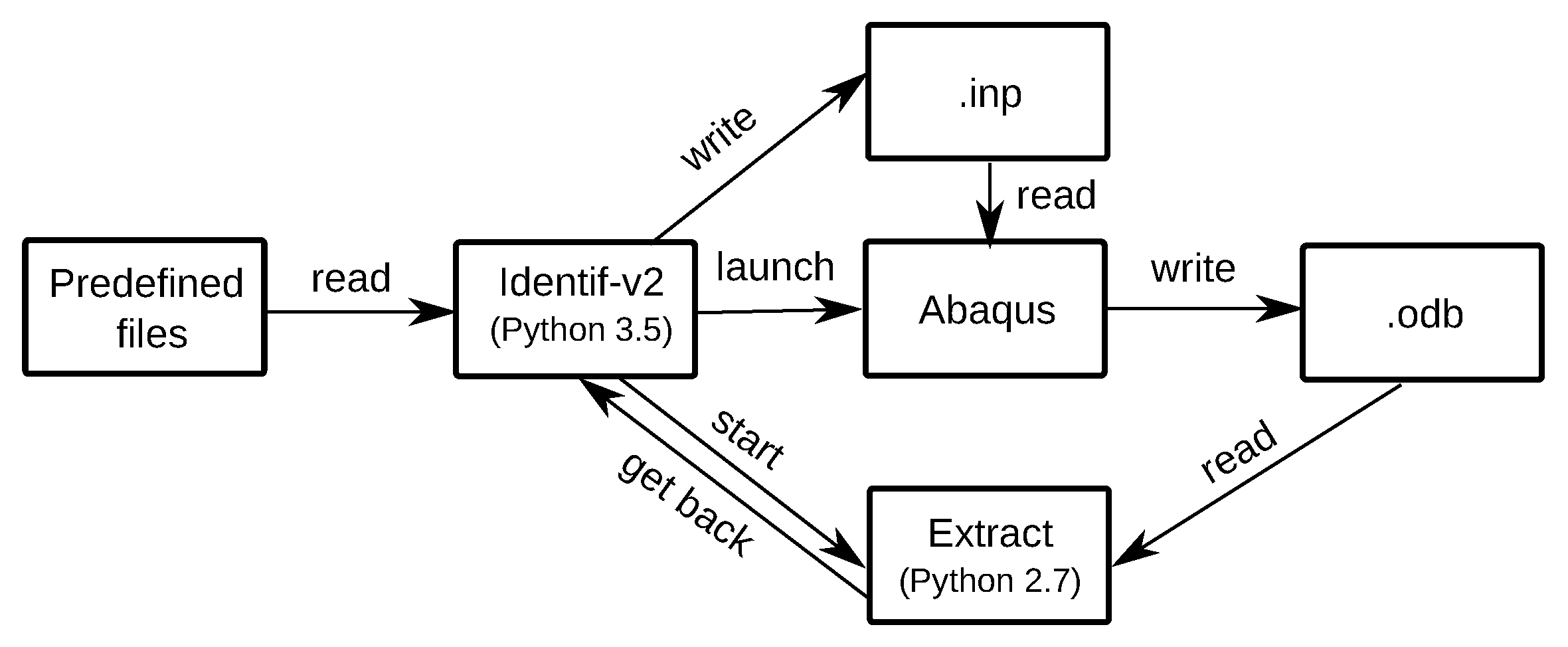
  • The first is to extract these numerical responses from the output database file (.odb) generated by Abaqus Explicit. As the identification program is a repeated testing process, it generates a large amount of numerical responses. The work of extracting the data cannot rely on a manual operation. Instead, the required data must be extracted automatically from the file .odb. Thus, a data extraction program called Extract is proposed. The implementation of the extractor is performed in a different script file from the main program, Identif-v2, because the identification program is written in Python3, while the Extract program is written in Python2 (Abaqus only accepts Python2 script files, and we have to explore the Abaqus .odb database).
  • The second question is how to achieve accurate numerical answers in a short computation time. We found that the responses extracted from the .odb file are not constant but oscillate in time (due to elastic waves inside the specimens). If we want to obtain stable responses, we have to spend a lot of time in the simulation (after having introduced an artificial damping to absorb these elastic waves). As one of our goals is to improve the efficiency of the identification program, long simulations should be avoided. To obtain the approximation of stable responses in a short simulation time, a data estimation method has been developed and implemented in the program Identify-v2.

3.1. Data Extraction from .odb Files

To automatically extract the numerical responses from the file .odb generated by Abaqus Explicit, a program named Extract written in Python2 language is proposed. The execution of this program is controlled by Identif-v2. We use it when the numerical simulation of Abaqus Explicit is finished, and it mainly deals with extracting some selected results and performing some basic operations from the output history of .odb. It is used to extract the geometric positions of selected nodes from the numerical model. This program can also calculate certain geometric parameters at certain locations in the numerical model using certain interpolation methods. The time evolution of these numerical responses is stored in an output file, and we will use the contents of this file in the data estimation step described below.

3.2. Data Estimation

The responses extracted from the file .odb cannot be used directly for the identification procedure. Due to the Abaqus Explicit algorithm and the nature of the simulated process, these responses are not constant but oscillate with time mainly due to the presence of elastic waves propagating inside the specimen during the calculation.
As an illustration, below we take the example of the dynamic tensile test. In this test, we launch a projectile to impact a specially designed target, and the tensile deformation occurs mainly in the useful area of the tensile target. This test is simulated with Abaqus Explicit, and the schematic of the numerical model is shown in Figure 3. More details on the dynamic tensile test are presented in Section 4.2. The impact velocity of the projectile is set to 75 m/s. The five dimensions shown in Figure 4 are selected as numerical responses.
The evolution of the geometric response H 10 as a function of time extracted by the program Extract is shown in Figure 5. As the simulation time increases, the oscillations decrease and the stable result can finally be obtained, but the calculation takes a long time. To improve the efficiency of the identification program, a method to estimate the stable responses in a short simulation time is proposed in this section and validated in Section 3.3.

3.2.1. Data with High Frequency Oscillations

The first step is to filter out the high frequency oscillations of the output signal. This first step is mandatory due to the procedure used to estimate long-term stable responses. A Savitzky–Golay digital filter [17,18] is used. It can be applied to smooth a series of data points, i.e., increase the signal-to-noise ratio without distorting the signal. It smooths the data by fitting successive subsets of adjacent data points with a low degree polynomial using the linear least squares method.
The Savitzky–Golay filter can be used directly in Python language, as it is implemented natively in the Python library scipy. It requires the definition of two parameters: the window length M (M must be a positive odd integer) and the polynomial order N, where N is chosen considerably smaller than M to obtain more smoothness and numerical stability. As the total number of data points T P is defined as a function of the time step and the requested output frequency, it is impossible to propose a fixed value of M a priori for all types of numerical models. We therefore proposed to define a ratio between M and T P to compute the window length for all types of models. In our case, the proposed ratio is set to M T P 1 40 and the order is set to N = 1 .
Figure 6 shows the result of high frequency filtering for H 10 of the dynamic pull target, where the red curve represents the original response and the blue curve the filtered response. To be more precise, the circular area on the left is enlarged and shown on the right, where the oscillations of the original data are replaced by an extreme point of the filtered data. We can now use the filtered and smoothed blue signal for the estimation of the long-term stable response.

3.2.2. Data with High Frequency Oscillations

Thanks to the Savitzky–Golay filter, the high frequency oscillations are now removed from the original response. However, the low frequency oscillations still exist. The example is represented by the blue curve in Figure 7, which is the time variation of the geometric distance H 10 for the dynamic traction target already filtered by the Savitzky–Golay filter. Therefore, the next problem is how to estimate the stable response of the data with low frequency oscillations using the least amount of simulation time. As the filtered response is a smooth decay curve, the average of the extreme points can be used as an estimate of the stable response, which is represented by the red line in Figure 7. The method for estimating the stable response is shown as follows.
At least five extreme points are needed in each type of filtered response, and we found that the average value of the first two extreme points, from the right, is close to the stabilized response. Therefore, their average can be the approximation of the steady state.The five extreme points required for the time variation of the geometric distance H 10 were plotted in Figure 7. This was optimized by testing to reduce the required computational time.

3.3. Validation of the Data Estimation Method

The simulation of the dynamic tensile test is still used to validate the data estimation method proposed above. Thus, for this validation process, two simulation times t were chosen ( t = 300 µs and t = 0.1 s). Here, the numerical damping associated with the explicit time integration scheme and used to stabilize the solution reduces the amplitude of the oscillations with time leading to a stabilized response after a long simulation time.
  • The first value t = 0.1 s is considered long enough to obtain stable responses of the geometrical parameters. The simulation process in this case takes about 5 hours of computation.
  • The second value t = 300 µs is used to obtain geometric responses in a short computation time which is less than 1 minute of simulation, although these geometric responses are not stabilized at the end of the computation as seen earlier.
The predefined impact velocity is set to 75 m/s. For the geometric responses obtained in these two cases, their approximations are computed using the data estimation method and reported with the stable responses in the Table 1. The approximations of the simulated responses with t = 0.1 s and t = 300 µs are denoted as A L (Approximated solution Long) and A S (Approximated solution Short), respectively. Therefore, the errors between the stable responses and A L are denoted by Δ L , and the errors between the stable responses and A S are denoted by Δ S .
We first compare A L with the stable responses. As we can see, each term of D e l t a L is 0.00 % . The stable responses and A L are identical. This means that we do not introduce any error by the proposed data estimation method. Next, we compare A S with the stable responses. The maximum error appears in the geometric response of H 10 , whose value is 0.18 % . The minimum error appears in the geometric response of H T with the value of 0.00 % . Although not all terms of Δ S are 0.00 % , the accuracy of A S is in an acceptable range, which means that the proposed data estimation method can estimate the stabilized responses in a short simulation time.
In conclusion, the proposed data estimation method has been validated by the dynamic tensile test. It can achieve the balance between efficiency and accuracy during computation, considering the huge difference in computational cost (5 h vs. 1 min) and minor errors (maximum 0.18 % ) between the stable and A S responses.

4. Applications of the Inverse Identification Procedure

In this section, the effectiveness of the proposed identification procedure is validated by identifying the equivalent impact velocities for the simplified models of the Taylor test, dynamic tensile test, and dynamic shear test. The materials used for the numerical models include 42CrMo4 steel, 2017-T3 aluminum, and polycarbonate, and their properties are listed in Table 2.

4.1. Simulation of the Taylor Test

The Taylor test is generally referred to as the Taylor impact test in other works [3,21]. In this test, a flat-ended cylindrical specimen is launched, normally with a prescribed impact velocity toward a target to induce deformation. The projectile used in the Taylor test is a cylinder of 50 mm length and 10 mm diameter ( L / D = 5 ). After it is launched at a rigid target, large deformations and high strain rates are generated in the region near the impacted end of the projectile. This shortens the projectile in a non-uniform manner, manifesting a mushroom head at the impacted end [22]. The dimensions of the projectile shoe, used to guide the projectile into the barrel of the gas gun, are shown in Figure 8. The same target support, whose geometry is shown in Figure 9, is used for all experimental tests. In the Taylor test, a 10 mm thick and 30 mm diameter cylindrical disk made of C100 steel is attached to the left side of the target holder to serve as a rigid target.

4.1.1. The Complete Model and Simplified Model

The full 2D axisymmetric model (referred to as C-M hereafter) simulates the Taylor test as shown in Figure 10, including a polycarbonate sabot, a 2017-T3 aluminum projectile, and a 42CrMo4 steel target holder. As it is impossible to construct the 2D axisymmetric model for the sabot, in this case, the sabot is replaced by a cylinder of the same mass, with a height of 25 mm, a radius of 5 mm, and a ρ density of 6.11 g/cm 3 . To simulate the real boundary condition, the axial displacement of the target support is free during impact. A predefined velocity of V c = 287 m/s along the z axis is imposed on the projectile and sabot. The sabot, the projectile, and the target support are made of 500, 1625, and 2235 CAX4RT elements, respectively. The total simulation time is t = 80 µs.
The simplified 2D axially symmetric model (referred to as C-M hereafter) consists of only a cylindrical shoe (500 CAX4RT elements) and a projectile (1625 CAX4RT elements), as shown in Figure 10. We simulate the simplified model under the same loading conditions as the full model, except for the boundary conditions. To simulate the contribution of the massive target support, we limit the axial displacement on the left side of the projectile while the radial displacement is free (this corresponds to a perfect frictionless contact of the projectile on the target).
The equivalent plastic strain contours of the projectile for the full model and the simplified model are plotted in Figure 11. Both models have fairly similar strain distributions, and the maximum strain occurs in the lower part of the projectile. Table 3 reports the values of the maximum equivalent plastic strain ε p and some geometric results, including the final length L f , final bottom radius R f , radii R 10 , R 20 , and R 30 at heights of 10 mm, 20 mm, and 30 mm from the contact tip, respectively.
As can be seen, these simplifications lead to some errors in the simulation results if the same loading conditions are used for the full model and the simplified model, hence the need to adjust the boundary conditions when switching from the full model to the simplified model.

4.1.2. Equivalent Loading Conditions for the Taylor Test

It may be mentioned that as the full model is built to simulate real impact conditions, the axial displacement of the target support is not fixed during impact. This means that the projectile and the target support in the full model are not stationary after impact. Instead, they are still moving in the impact chamber with a residual velocity of V r = 2.26 m/s. The same is true in the experiments because the target is not fixed and is free to move after impact to avoid damage from the impact energy. However, the target for the simplified model is fixed to simulate the contribution of the massive target support. This change will introduce errors in the numerical simulations if we use the same impact velocity for the full model and the simplified model. To obtain more accurate simulation results, we need to take into account the residual kinetic energy of the projectile and the target support. Thus, an adjusted impact velocity must be used when the Taylor test is simulated with the simplified model.
Therefore, the proposed inverse identification procedure is used to identify the equivalent impact velocity for the simplified model by minimizing the difference between the final deformed shape of the full model and the final deformed shape of the simplified model. Initially, the full model and the simplified model were simulated with the original impact velocities between 30 m/s and 240 m/s, and then the simplified model was simulated again with the impact velocities proposed by the identification procedure. Their computation times and geometric responses are compared in the Table 4. To reduce the length of the table, we omit the results with original velocities of 60 m/s, 150 m/s, and 210 m/s.
As the simplified model has fewer elements to calculate, the computational time of the simplified model is less than that of the full model by a factor of about 28.6 % . As for the geometric responses, the differences between the full model and the simplified model are generally reduced by using the equivalent velocities. This study allows us to identify a linear function for estimating the equivalent velocity V S when the original impact velocity V R from the Taylor test is determined, which has the following expression:
V S = 1.00448 V R 1.45767

4.2. Simulation of the Dynamic Tensile Test

To characterize the behavior of materials subjected to dynamic tension, the Taylor impact technique was initially extended in the LGP [10], which is referred to as the dynamic tension test in this work. In this test, the Taylor gas gun device is used to launch a projectile into a specially designed target with different impact velocities, and tensile deformation occurs primarily in the central region of the target. We have modified the geometry of the tensile target, compared to the previous version, and optimized it to achieve higher deformations and elongation without reaching the critical state of target failure [23]. The optimized target has the geometry shown in Figure 12. The projectile made by assembling an axisymmetric polycarbonate sabot and a 42CrMo4 steel head has the geometry shown in Figure 13. The right side of the target support shown in Section 4.1 is used to support the target during the dynamic tensile test.

4.2.1. The Complete Model and Simplified Model

The complete 2D axisymmetric model of the dynamic tensile test is shown in Figure 14, consisting of four parts: a polycarbonate sabot, a 42CrMo4 steel impactor head, a 2017-T3 aluminum target, and a 42CrMo4 steel target holder. A predefined velocity of V c = 70 m/s along the z axis is imposed on the projectile and the sabot. To simulate the real boundary condition, the axial displacement of the target support is free during impact. The sabot, projectile, pull target, and target support consist of 169, 240, 3814, and 2190 CAX4RT elements, respectively. The total simulation time is t = 300 µs. We propose a simplified model to replace the full model. (240 CAX4RT elements) and a target (2190 CAX4RT elements), as shown in the lower part of Figure 14.
We fix the axial displacement of the top of the target to simulate the contribution of the massive target support. We consider the contribution of the sabot in the simulation by adding the mass of the sabot on the projectile instead of building the numerical model of the sabot, thus the density of the projectile ρ = 10,760 kg/m 3 .
Figure 15 shows the contour plot of the equivalent plastic strain of the tensile target for the full model and the simplified model. The strain distributions for both models are the same. The maximum equivalent plastic strains are concentrated in their useful areas, and the difference between the maximum values is 3.21 % .
Table 5 shows the geometric responses for both models, including three of dimensions along the axial direction ( H 10 , H M , and H T ) and two of dimensions along the radial dimension ( R I and R E ) as presented in Figure 4. The differences in responses between C-M and S-M show that these simplifications lead to some errors as presented earlier.

4.2.2. Equivalent Loading Conditions for the Dynamic Tensile Test

Similar to the Taylor test simulation, we need to use an equivalent impact velocity for the simplified dynamic tensile test model to account for the residual kinetic energy of the target and its support. The proposed inverse identification procedure is again used to identify the equivalent impact velocity.
Table 6 reports the geometric responses of the full model and the simplified model with original impact velocities ranging from 60 m/s to 75 m/s, and the simplified model with the impact velocities proposed by the identification procedure. Differences in geometric responses between the full model and the simplified model are obviously reduced by using the equivalent identified velocities.
As previously proposed, a linear function giving the equivalent velocity V S as a function of the original impact velocity V R , can be identified:
V S = 1.00618 V R 2.1419

4.3. Simulation of the Dynamic Shear Test

In addition to the dynamic tensile test, the Taylor impact technique has also been extended to the dynamic shear test in the LGP laboratory [8]. We perform the dynamic shear test in the same manner as the dynamic tensile test, except that the geometry of the shear target differs from the tensile target. The projectile, shoe, and target holder for the dynamic shear test are identical to those used for the dynamic tensile test. The shear target, referred to as a hat-shaped specimen, has a geometry as shown in Figure 16. It can be divided into three regions: the upper part of the hat, the lower part of the brim, and the shear region, where the large shear strains develop.

4.3.1. The Complete Model and Simplified Model

The complete 2D axisymmetric model is established as shown in Figure 17, including a polycarbonate sabot, a 42CrMo4 steel projectile, a 2017-T3 aluminum target, and a 42CrMo4 steel target holder. A predefined velocity of V c = 45 m/s along the z axis is imposed on the projectile and sabot, and the axial displacement of the target holder is free during impact. The sabot, projectile, shear target, and target holder consist of 131, 233, 4457, and 2223 CAX4RT elements, respectively. The total simulation time is t = 100 µs.
We propose the simplified model of the dynamic shear test to reduce the computational cost, which includes only a projectile (233 CAX4RT elements) and a target (4457 CAX4RT elements). This simplified model is simulated under the same loading conditions as the full model, except that the axial displacement of the top of the shear target is fixed to simulate the contribution of the massive target support, as shown in Figure 17. Similar to the dynamic tensile test simulation, we changed the density to ρ = 10,760 kg/m 3 .
The equivalent plastic strains of the simplified model and the full model are compared in Figure 18. These two models show similar strain distributions: a zone where the material is mainly deformed in shear exists due to the specific geometry of the specimen, and strain localization also occurs in this zone. In terms of maximum equivalent plastic strain ε p , the difference between these two models is significant ( 22.51 % ).
Table 7 reports the results of the more global responses along the axial direction, H T and H M as presented in Figure 17. As we can see, the simplifications lead to some errors in the simulation results if we use the same loading conditions for the full model and the simplified dynamic shear test model.

4.3.2. Equivalent Loading Conditions for the Dynamic Tensile Test

We applied the same procedure to identify an equivalent impact velocity for the simplified model. Table 8 reports the geometric responses of the full model and the simplified model with original impact velocities ranging from 25 m/s to 45 m/s, and the simplified model with impact velocities proposed by the identification procedure. The discrepancy in geometric responses between the full model and the simplified model is reduced by using the equivalent velocities.
Again, the relationship between the original velocities for the full model and the corresponding equivalent velocities for the simplified model can be considered linear. The fitting function giving the equivalent velocity V S as a function of the original impact velocity V R can be written as follows:
V S = 0.89988 V R + 0.1066

5. Conclusions

In this paper, we have proposed an inverse identification procedure to evaluate equivalent loading conditions for simplified numerical models in Abaqus Explicit. We have developed a robust and stable identification program in Python language, where the Levenberg–Marquardt algorithm is employed to minimize the differences between the final deformed shape of the full models and the final deformed shape of the simplified models. We proposed a Python program to automatically extract the numerical responses from Abaqus Explicit. Validated by the simulation of the dynamic tensile test, we applied a data estimation method to estimate the stable responses with short computation time. The proposed comprehensive equivalent boundary condition identification procedure was validated by identifying the equivalent impact velocities for the simplified models of the Taylor test, dynamic tensile test, and dynamic shear test. We proved the need to identify equivalent loading conditions for the simplified models in order to recalibrate their results to the full numerical models.

Author Contributions

Conceptualization, O.P.; methodology, O.P.; software, O.P.; validation, O.P. and L.M.; formal analysis, O.P. and L.M.; investigation, O.P. and L.M.; resources, O.P.; data curation, O.P. and L.M.; writing—original draft preparation, L.M.; writing—review and editing, O.P.; visualization, O.P. and L.M.; supervision, O.P.; project administration, O.P.; funding acquisition, O.P. All authors have read and agreed to the published version of the manuscript.

Funding

This research was funded by China Scholarship Council (CSC) under Grant number CSC n°201406290010.

Institutional Review Board Statement

Not applicable.

Informed Consent Statement

Not applicable.

Data Availability Statement

Data are accessible by contacting the corresponding author.

Conflicts of Interest

The authors declare no conflict of interest.

References

  1. Uhl, T. The inverse identification problem and its technical application. Arch. Appl. Mech. 2007, 77, 325–337. [Google Scholar] [CrossRef]
  2. Hendriks, M.A.N. Identification of the Mechanical Behavior of Solid Materials; Technische Universiteit Eindhoven: Eindhoven, The Netherlands, 1991. [Google Scholar]
  3. Nistor, I.; Pantalé, O.; Caperaa, S.; Sattouf, C. Identification of a dynamic viscoplastic flow law using a combined levenberg-marquardt and monte-carlo algorithm. In Proceedings of the VII International Conference on Computational Plasticity, COMPLAS, Barcelona, Spain, 7–10 April 2003. [Google Scholar]
  4. Cooreman, S.; Lecompte, D.; Sol, H.; Vantomme, J.; Debruyne, D. Identification of mechanical material behavior through inverse modeling and DIC. Exp. Mech. 2008, 48, 421–433. [Google Scholar] [CrossRef]
  5. Furukawa, T.; Sugata, T.; Yoshimura, S.; Hoffman, M. An automated system for simulation and parameter identification of inelastic constitutive models. Comput. Methods Appl. Mech. Eng. 2002, 191, 2235–2260. [Google Scholar] [CrossRef]
  6. Nistor, I.; Pantalé, O.; Caperaa, S.; Sattouf, C. A new dynamic test for the identification of high speed friction law using a gas-gun device. J. Phys. IV (Proc.) 2003, 110, 519–524. [Google Scholar] [CrossRef]
  7. Nistor, I.; Pantalé, O.; Caperaa, S. A new impact test for the identification of a dynamic crack propagation criterion using a gas-gun device. J. Phys. IV (Proc.) 2006, 134, 713–718. [Google Scholar] [CrossRef] [Green Version]
  8. Sattouf, C. Caractérisation en Dynamique Rapide du Comportement de Matériaux Utilisés en Aéronautique. Ph.D. Thesis, INPT, Toulouse, France, 2003. [Google Scholar]
  9. Sattouf, C.; Pantalé, O.; Caperaa, S. A methodology for the identification of constitutive and contact laws of metallic materials under High Strain Rates. In Advances in Mechanical Behaviour, Plasticity and Damage; Elsevier: Tours, France, 2000; pp. 621–626. [Google Scholar]
  10. Abichou, H.; Pantalé, O.; Nistor, I.; Dalverny, O.; Caperaa, S. Identification of metallic material behaviors under high-velocity impact: A new tensile test. In Proceedings of the 15th Technical Meeting DYMAT, Metz, France, 1–2 June 2004; pp. 1–2. [Google Scholar]
  11. Gavrus, A.; Massoni, E.; Chenot, J. An inverse analysis using a finite element model for identification of rheological parameters. J. Mater. Processing Technol. 1996, 60, 447–454. [Google Scholar] [CrossRef]
  12. Lloyd, B.; Székely, G.; Harders, M. Identification of spring parameters for deformable object simulation. IEEE Trans. Vis. Comput. Graph. 2007, 13, 1081–1094. [Google Scholar] [CrossRef] [PubMed]
  13. Levenberg, K. A method for the solution of certain non-linear problems in least squares. Q. Appl. Math. 1944, 2, 164–168. [Google Scholar] [CrossRef] [Green Version]
  14. Marquardt, D. An Algorithm for Least-Squares Estimation of Nonlinear Parameters. J. Soc. Ind. Appl. Math. 1963, 11, 431–441. [Google Scholar] [CrossRef]
  15. Lourakis, M.I. A Brief Description of the Levenberg-Marquardt Algorithm Implemented by Levmar; Foundation of Research and Technology: Heraklion, Greece, 2005; Volume 4. [Google Scholar]
  16. Newville, M.; Stensitzki, T.; Allen, D.B.; Rawlik, M.; Ingargiola, A.; Nelson, A. LMFIT: Non-Linear Least-Square Minimization and Curve-Fitting for Python. Zenodo:10.5281/zenodo.5570790. 2021. Available online: https://ui.adsabs.harvard.edu/abs/2016ascl.soft06014N/abstract (accessed on 18 April 2022).
  17. Savitzky, A.; Golay, M.J. Smoothing and differentiation of data by simplified least squares procedures. Anal. Chem. 1964, 36, 1627–1639. [Google Scholar] [CrossRef]
  18. Guest, P.G. Numerical Methods of Curve Fitting; Cambridge University Press: Cambridge, UK, 2012. [Google Scholar]
  19. Sattouf, C.; Dalverny, O.; Rakotomalala, R. Identification and comparison of different constitutive laws for high speed solicitation. J. Phys. IV (Proc.) 2003, 110, 201–206. [Google Scholar] [CrossRef]
  20. Dwivedi, A.; Bradley, J.; Casem, D. Mechanical Response of Polycarbonate with Strength Model Fits; Technical Report; Dynamic Science Inc.: Aberdeen, MD, USA, 2012. [Google Scholar]
  21. Taylor, G. The use of flat-ended projectiles for determining dynamic yield stress. I. Theoretical considerations. Proc. R. Soc. Lond. Math. Phys. Eng. Sci. R. Soc. 1948, 194, 289–299. [Google Scholar]
  22. Sarva, S.; Mulliken, A.D.; Boyce, M.C. Mechanics of Taylor impact testing of polycarbonate. Int. J. Solids Struct. 2007, 44, 2381–2400. [Google Scholar] [CrossRef] [Green Version]
  23. Ming, L. A Numerical Platform for the Identification of Dynamic Non-Linear Constitutive Laws Using Multiple Impact Tests: Application to Metal Forming and Machining. Ph.D. Thesis, INPT, Toulouse, France, 2018. [Google Scholar]
Figure 1. Flow chart of Identif-v2.
Applmech 03 00039 g001
Figure 2. Data flow diagram of the proposed inverse identification procedure.
Applmech 03 00039 g002
Figure 3. The schematic diagram of dynamic tensile test.
Applmech 03 00039 g003
Figure 4. Dimensions to be measured for the dynamic tensile test.
Applmech 03 00039 g004
Figure 5. H 10 vs. time plot of the dynamic tensile test.
Applmech 03 00039 g005
Figure 6. The high frequency filtering for H 10 of dynamic tensile test.
Applmech 03 00039 g006
Figure 7. H 10 of dynamic tensile target with low frequency oscillations.
Applmech 03 00039 g007
Figure 8. Dimensions of the sabot for the Taylor test.
Applmech 03 00039 g008
Figure 9. Geometry of the target support for all experiments.
Applmech 03 00039 g009
Figure 10. Complete and simplified Taylor models.
Applmech 03 00039 g010
Figure 11. Equivalent plastic strain contour-plots of the complete model and simplified model for Taylor test. (a) Equivalent plastic strain contour-plot of the complete model; (b) Equivalent plastic strain contour-plot of the simplified model.
Applmech 03 00039 g011
Figure 12. The geometry of the target for the dynamic tensile test.
Applmech 03 00039 g012
Figure 13. The projectile for the dynamic tensile test and the Dynamic shear test.
Applmech 03 00039 g013
Figure 14. Complete and simplified dynamic tensile models.
Applmech 03 00039 g014
Figure 15. Equivalent plastic strain contour-plots of the complete model and simplified model for Dynamic tensile test. (a) Equivalent plastic strain contour-plot of the complete model; (b) Equivalent plastic strain contour-plot of the simplified model.
Applmech 03 00039 g015
Figure 16. Geometry of the target for the dynamic shear test.
Applmech 03 00039 g016
Figure 17. Complete dynamic shear model.
Applmech 03 00039 g017
Figure 18. Equivalent plastic strain contour-plots of the complete model and simplified model for dynamic shear test. (a) Equivalent plastic strain contour-plot of the complete model; (b) Equivalent plastic strain contour-plot of the simplified model.
Applmech 03 00039 g018
Table 1. Data processing results of the geometric parameters of the dynamic tensile test.
ResponseTime H 10 H M H T R I R E
(mm)(mm)(mm)(mm)(mm)
Stable 0.1  s 12.037 22.378 38.303 11.063 11.897
A L 0.1  s 12.037 22.378 38.303 11.063 11.897
Δ L 0.00 % 0.00 % 0.00 % 0.00 % 0.00 %
A S 300 µs 12.059 22.380 38.301 11.059 11.892
Δ S 0.18 % 0.01 % 0.00 % 0.04 % 0.04 %
Table 2. Material parameters of the 42CrMo4 steel [19], the 2017-T3 aluminum [8], and the polycarbonate [20].
42CrMo42017-T3Polycarbonate
E (Gpa) 206.9 72.4 2.59
ν 0.29 0.33 0.39
A (MPa)80636080
B (MPa)6143175
C 0.0089 0.0188 0.052
n 0.168 0.289 2
m 1.1 0.96 0.548
ε 0 .  (s 1 )111
T 0  (°C)202020
T m  (°C)1540513289
ρ  (kg/m 3 )783027901220
λ  (W/m°C) 34.0 134 0.163
C p  (J/kg°C)4608801200
η 0.9 0.9 0.9
Table 3. Comparison between the complete model (C-M) and simplified model (S-M) for Taylor compression test.
ε p L f R f R 10 R 20 R 30
(mm)(mm)(mm)(mm)(mm)
C-M 1.994 39.18 8.83 5.73 5.28 5.08
S-M 1.964 39.09 8.80 5.75 5.28 5.09
Δ 1.50 % 0.23 % 0.34 % 0.35 % 0.00 % 0.20 %
Table 4. Identification of the equivalent impact velocity V S for the simplified model of the Taylor test.
NumericalVelocity L f R f R 10 R 20 R 30 Δ
Model(m/s)(mm)(mm)(mm)(mm)(mm)
C-M30 49.94 5.01 5.01 5.01 5.00
S-M ( V R )30 49.96 5.00 5.00 5.00 5.00
Δ ( V R ) 0.04 % 0.08 % 0.01 % 0.09 % 0.01 % 0.02 %
S-M ( V S ) 29.963 49.96 5.00 5.00 5.00 5.00
Δ ( V S ) 0.04 % 0.08 % 0.01 % 0.09 % 0.01 % 0.02 %
C-M90 48.91 5.26 5.12 5.03 5.01
S-M ( V R )90 48.82 5.27 5.14 5.03 5.01
Δ ( V R ) 0.17 % 0.25 % 0.29 % 0.09 % 0.05 % 0.09 %
S-M ( V S ) 87.399 48.89 5.25 5.13 5.03 5.01
Δ ( V S ) 0.03 % 0.09 % 0.14 % 0.18 % 0.04 % 0.05 %
C-M120 48.01 5.50 5.23 5.05 5.01
S-M ( V R )120 47.94 5.52 5.23 5.05 5.01
Δ ( V R ) 0.14 % 0.30 % 0.06 % 0.06 % 0.04 % 0.07 %
S-M ( V S ) 118.787 47.98 5.50 5.23 5.05 5.01
Δ ( V S ) 0.06 % 0.03 % 0.01 % 0.05 % 0.12 % 0.03 %
C-M180 45.58 6.25 5.45 5.12 5.02
S-M ( V R )180 45.52 6.26 5.45 5.13 5.02
Δ ( V R ) 0.12 % 0.19 % 0.09 % 0.08 % 0.04 % 0.05 %
S-M ( V S ) 179.130 45.57 6.25 5.45 5.12 5.02
Δ ( V S ) 0.03 % 0.03 % 0.03 % 0.03 % 0.00 % 0.01 %
C-M240 42.41 7.48 5.63 5.22 5.05
S-M ( V R )240 42.34 7.49 5.65 5.22 5.05
Δ ( V R ) 0.17 % 0.16 % 0.26 % 0.08 % 0.02 % 0.07 %
S-M ( V S ) 239.970 42.34 7.49 5.65 5.22 5.05
Δ ( V S ) 0.17 % 0.15 % 0.26 % 0.08 % 0.01 % 0.07 %
Table 5. Comparison between the complete model (C-M) and simplified model (S-M) for dynamic tensile test.
ε p H 10 H M H T R I R E
(mm)(mm)(mm)(mm)(mm)
C-M 0.218 11.54 22.05 37.78 11.20 12.08
S-M 0.225 11.71 22.01 37.87 11.17 12.05
Δ 3.21 % 1.44 % 0.20 % 0.24 % 0.28 % 0.25 %
Table 6. Identification of the equivalent impact velocity for the simplified model of dynamic tensile test.
NumericalVelocity H 10 H M H T R I R E Δ
Model(m/s)(mm)(mm)(mm)(mm)(mm)
C-M60 11.02 21.47 37.07 11.41 12.33
S-M ( V R )60 11.16 21.41 37.15 11.38 12.31
Δ ( V R ) 1.27 % 0.28 % 0.22 % 0.26 % 0.16 % 0.27 %
S-M ( V S ) 58.145 11.09 21.30 37.02 11.42 12.35
Δ ( V S ) 0.64 % 0.79 % 0.13 % 0.09 % 0.16 % 0.21 %
C-M65 11.28 21.76 37.41 11.30 12.21
S-M ( V R )65 11.43 21.69 37.50 11.27 12.18
Δ ( V R ) 1.33 % 0.32 % 0.24 % 0.27 % 0.25 % 0.29 %
S-M ( V S ) 63.150 11.32 21.59 37.39 11.31 12.22
Δ ( V S ) 0.35 % 0.78 % 0.05 % 0.09 % 0.08 % 0.17 %
C-M70 11.54 22.05 37.78 11.20 12.08
S-M ( V R )70 11.71 22.01 37.87 11.17 12.05
Δ ( V R ) 1.47 % 0.18 % 0.24 % 0.27 % 0.25 % 0.31 %
S-M ( V S ) 68.236 11.61 21.90 37.75 11.20 12.10
Δ ( V S ) 0.61 % 0.68 % 0.08 % 0.00 % 0.17 % 0.19 %
C-M75 11.86 22.40 38.18 11.10 11.94
S-M ( V R )75 12.06 22.38 38.30 11.06 11.89
Δ ( V R ) 1.69 % 0.09 % 0.31 % 0.36 % 0.42 % 0.36 %
S-M ( V S ) 73.189 11.93 22.27 38.15 11.10 11.95
Δ ( V S ) 0.59 % 0.58 % 0.08 % 0.00 % 0.08 % 0.17 %
Table 7. Comparison between the complete model (C-M) and simplified model (S-M) for dynamic shear test.
ε p H T H M
(mm)(mm)
C-M 1.084 24.68 14.70
S-M 1.328 24.59 14.60
Δ 22.51 % 0.36 % 0.63 %
Table 8. Identification of the equivalent impact velocity for the simplified model of dynamic shear test.
Numerical ModelVelocity H T H M Δ
(m/s)(mm)(mm)
C-M25 24.95 14.95
S-M ( V R )25 24.93 14.92
Δ ( V R ) 0.08 % 0.19 % 0.10 %
S-M ( V S ) 22.361 24.96 14.95
Δ ( V S ) 0.02 % 0.03 % 0.02 %
C-M30 24.91 14.91
S-M ( V R )30 24.87 14.88
Δ ( V R ) 0.13 % 0.21 % 0.12 %
S-M ( V S ) 27.504 24.91 14.91
Δ ( V S ) 0.00 % 0.01 % 0.005 %
C-M35 24.85 14.86
S-M ( V R )35 24.77 14.80
Δ ( V R ) 0.31 % 0.38 % 0.25 %
S-M ( V S ) 31.496 24.85 14.86
Δ ( V S ) 0.01 % 0.00 % 0.005 %
C-M40 24.77 14.78
S-M ( V R )40 24.70 14.71
Δ ( V R ) 0.30 % 0.51 % 0.30 %
S-M ( V S ) 36.082 24.77 14.78
Δ ( V S ) 0.01 % 0.00 % 0.005 %
C-M45 24.68 14.70
S-M ( V R )45 24.59 14.60
Δ ( V R ) 0.36 % 0.63 % 0.36 %
S-M ( V S ) 40.569 24.69 14.70
Δ ( V S ) 0.02 % 0.02 % 0.01 %
Publisher’s Note: MDPI stays neutral with regard to jurisdictional claims in published maps and institutional affiliations.

