Selection Criteria for Biplane Wing Geometries by Means of 2D Wind Tunnel Tests

 , , ,
, , ,
Abstract
:1. Introduction
2. Materials and Methods
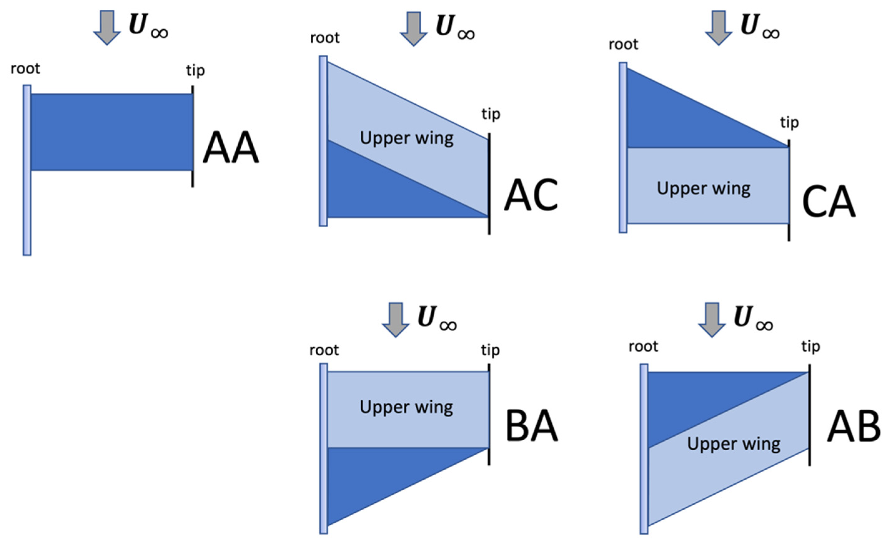
2.1. Prototypes Description
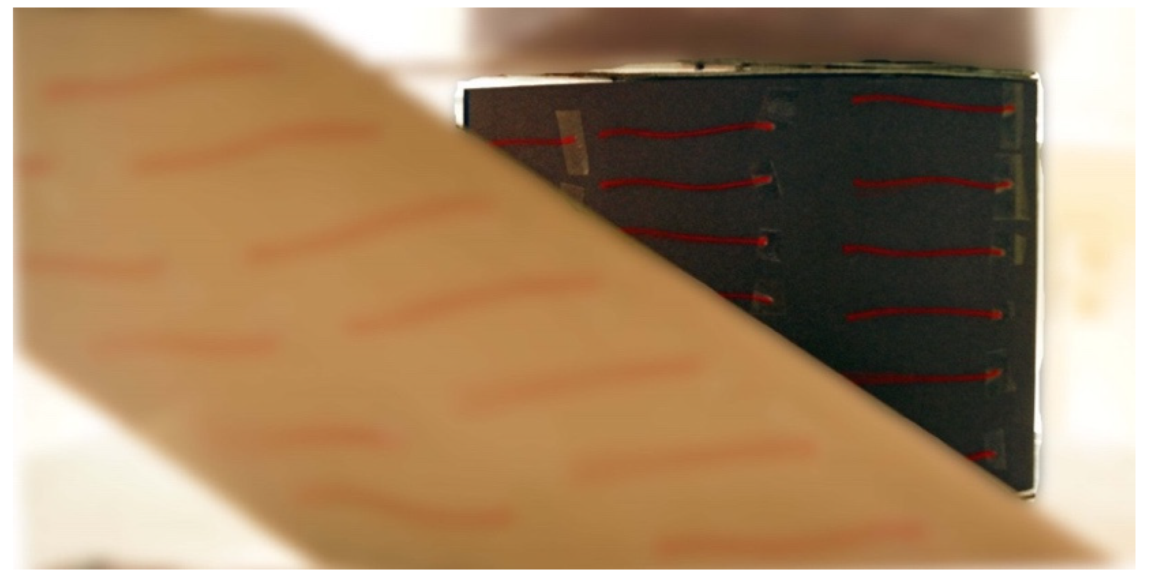
2.2. Wind Tunnel Facility
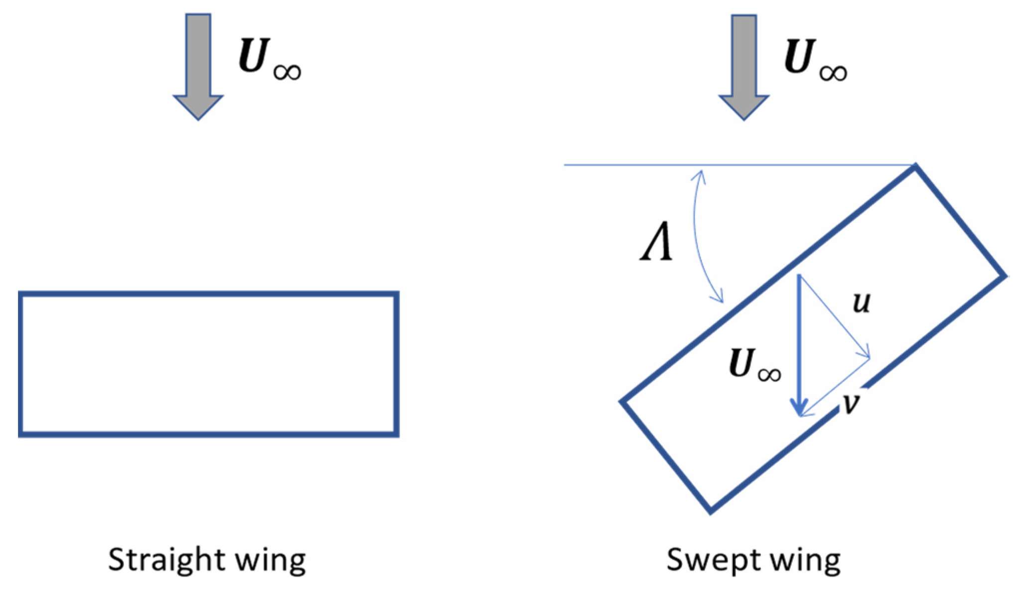
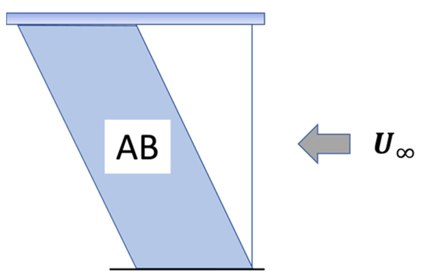
2.3. The Two–Dimensional Flow Hypothesis
2.4. Experimental Test Procedure
3. Results
4. Discussion
5. Conclusions
- increases with G.
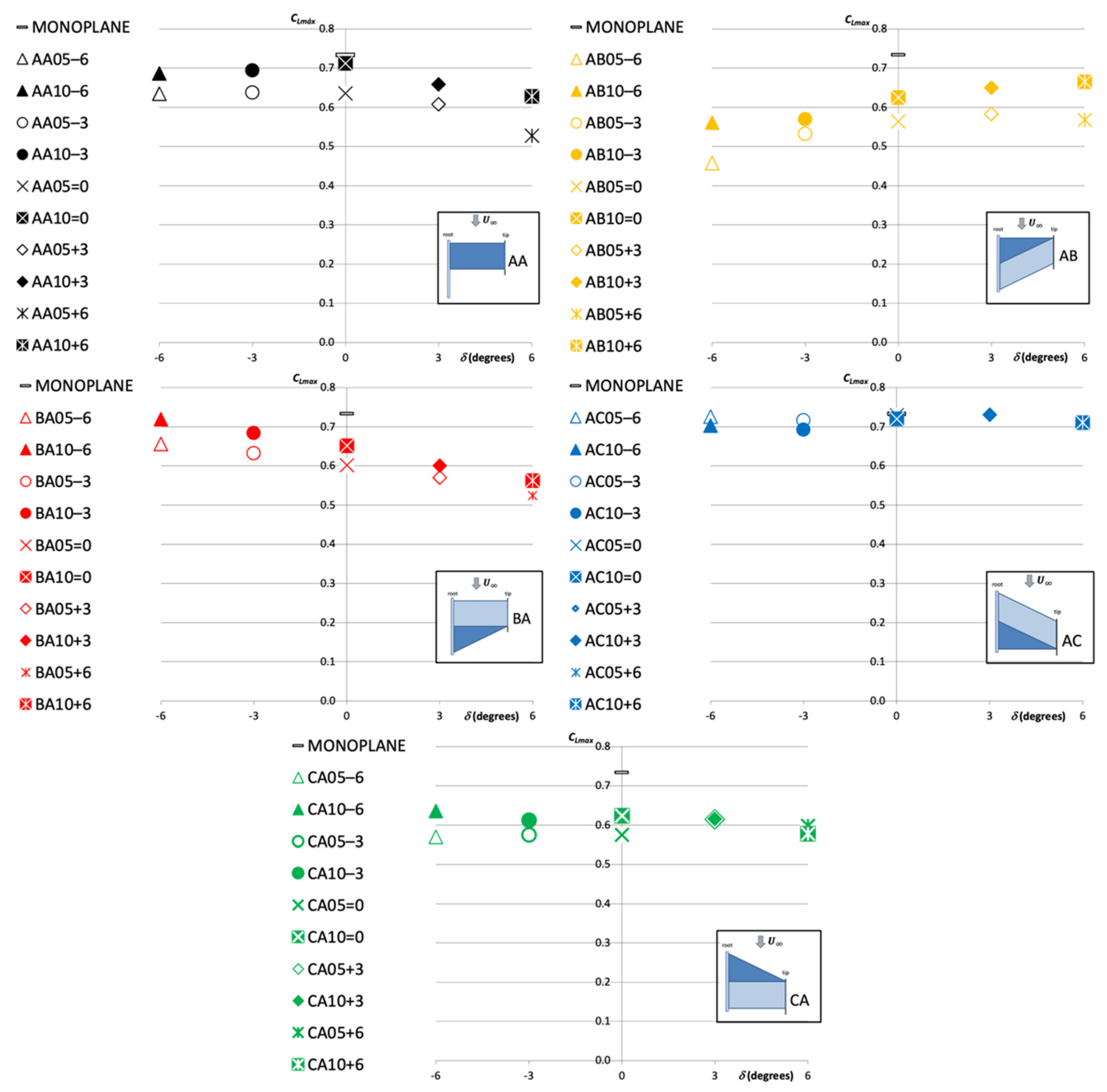
- For those wing configurations where , there is a relationship between and that depends on the wing configuration. For those configurations where , decreases asincreases. On the contrary, for the wing configuration where , the increases asincreases.
- For those wing configurations where the wing’s swept angle was , seems to remain constant with .
- seems to remain nearly constant.
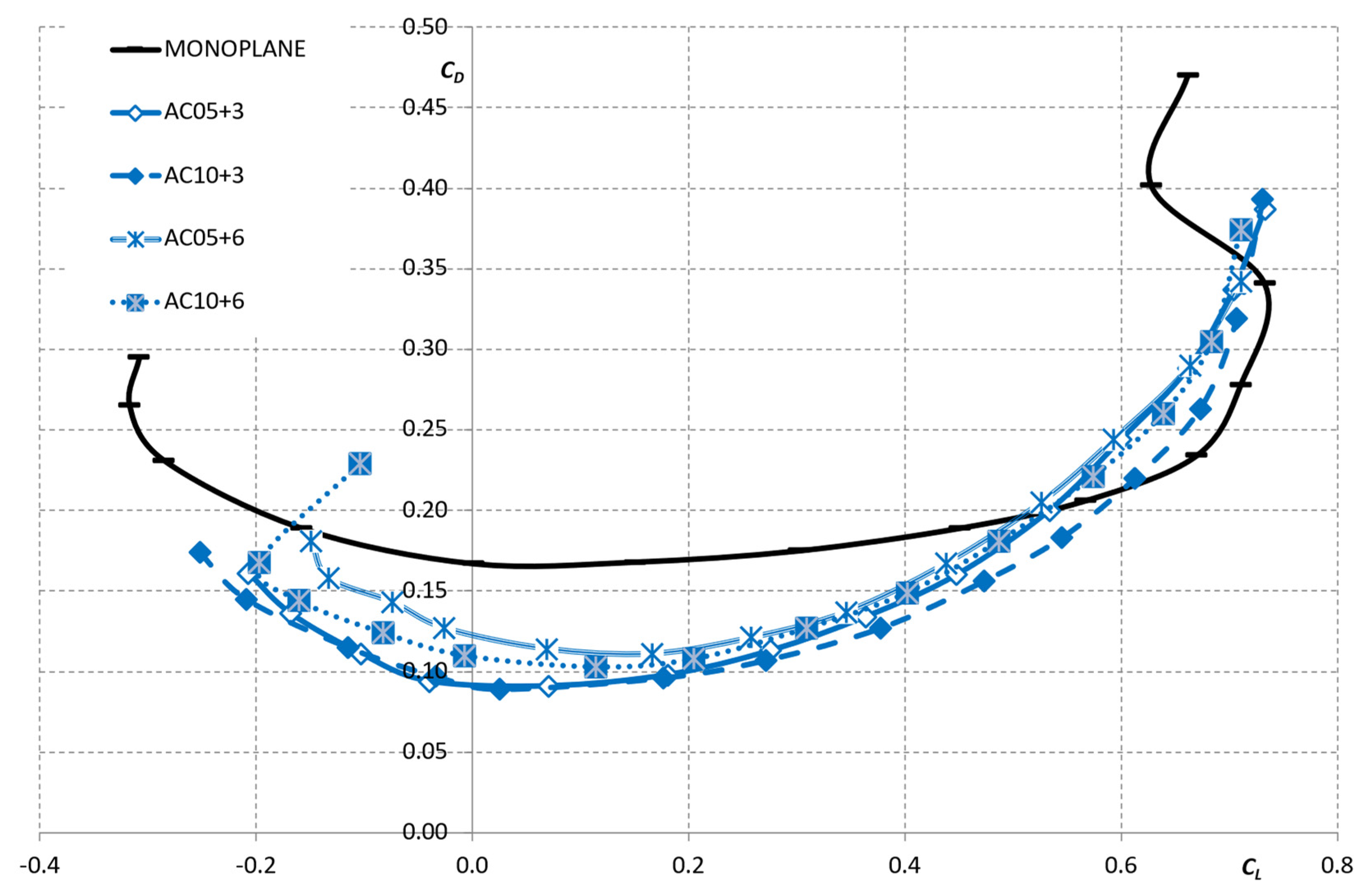
- A linear relationship between the and is evidenced for most of the cases. For those wing configurations where s < 0, the increase in seems to be greater. However, the overall higher values of are observed for those wing configurations with .
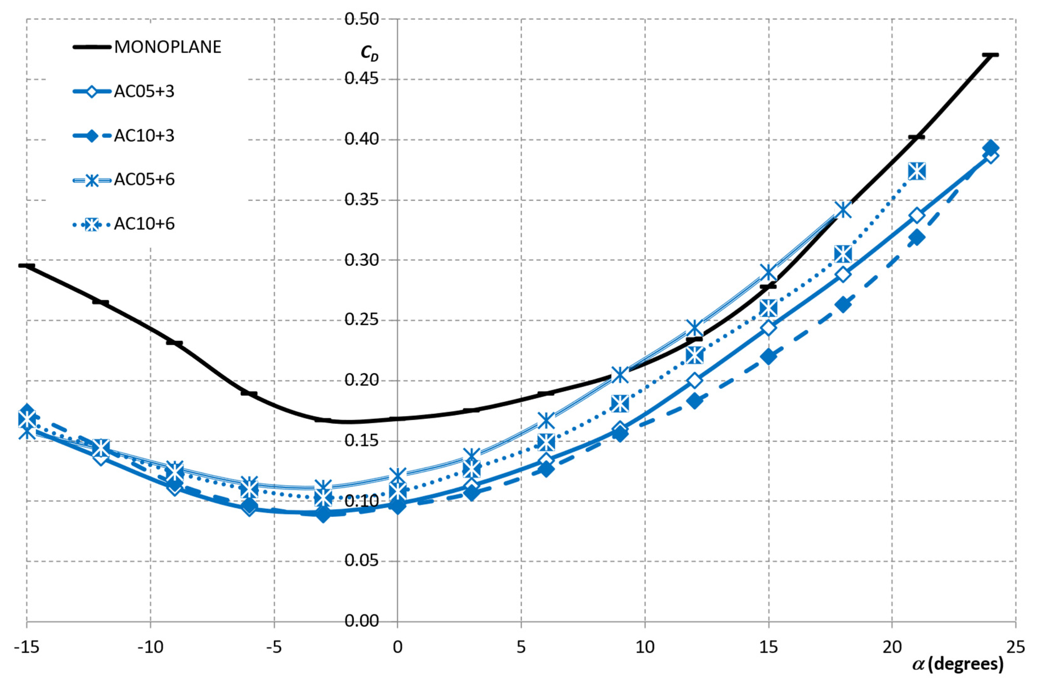
- The minimum value of are usually obtained for .
- As increases, the value of decreases.
Author Contributions
Funding
Institutional Review Board Statement
Informed Consent Statement
Data Availability Statement
Conflicts of Interest
Abbreviations
| The following abbreviations are used in this manuscript: | |
| MAV | Micro Air Vehicles |
| PIV | Particle Image Velocimetry |
| RMS | Root mean square |
| RPAS | Remotely Piloted Aircraft System |
| UAV | Unmanned Air Vehicle |
| The following nomenclature is used in this manuscript: | |
| AR | |
| b | Wingspan |
| c | Wing chord length |
| CL | |
| Lift slope coefficient | |
| CLo | Lift coefficient for zero angle of attack |
| CLmax | Maximum lift coefficient |
| CD | |
| CDO | Parasitic drag coefficient |
| CDi | Induced drag coefficient; drag due to lift |
| CDmin | Minimum profile drag coefficient |
| CL/CD | Lift–to–drag ratio |
| D | Drag |
| Induced drag | |
| Parasitic drag | |
| Drag due to lift | |
| E | Endurance. The time that an aircraft can fly between takeoff and landing based on several flight conditions. |
| Emax | Maximum endurance |
| G | Gap |
| Iu | . |
| L | Lift |
| R | Range. Distance an aircraft can fly between takeoff and landing based on several flight conditions. |
| Rmax | Maximum range |
| Re | |
| S | Wing gross area |
| s | Stagger |
| Mean value of air speed | |
| Umax | Maximum value of air speed on wind tunnel test section |
| Umin | Minimum value of air speed on wind tunnel test section |
| Freestream velocity | |
| xmax | Maximum horizontal distance in gliding flight. Distance that an aircraft can glide in a gliding flight based on several flight conditions. |
| W | Weight |
| Angle of attack | |
| Angle of attack for the minimum drag coefficient | |
| Increment in the profile drag coefficient due to lift | |
| Angle of incidence of each profile | |
| Air density | |
| Dynamic viscosity of air | |
| Standard deviation of U | |
| Sweep angle | |
References
- Munk, M.M. The Minimum Induced Drag of Airfoils; NACA TR 121; US Government Printing Office: Washington, DC, USA, 1923. [Google Scholar]
- Prandtl, L. Induced Drag of Multiplanes; NACA TN 182; US Government Printing Office: Washington, DC, USA, 1924. [Google Scholar]
- Jemitola, P.O.; Fielding, J.P. Box Wing Aircraft Conceptual Design. In Proceedings of the 28th Congress of the International Council of the Aeronautical Sciences, Brisbane, Australia, 23–28 September 2012; pp. 1–10. Available online: http://www.icas.org/ICAS_ARCHIVE/ICAS2012/PAPERS/213.PDF (accessed on 7 March 2022).
- Jemitola, P.O.; Monterzino, G.; Fielding, J. Wing mass estimation algorithm for medium range box wing aircraft. Aeronaut. J. 2013, 117, 329–340. [Google Scholar] [CrossRef]
- Kroo, I. Nonplanar wing concepts for increased aircraft efficiency. VKI Lect. Ser. Innov. Config. Adv. Concepts Futur. Civ. Aircr. 2005, 1, 6–10. [Google Scholar]
- Khan, F.; Krammer, P.; Scholz, D. Preliminary Aerodynamic Investigation of Box–Wing Configurations Using Low Fidelity Codes. Dtsch. Luft– und Raumfahrtkongress Doc. 2010, 161308, 313–327. [Google Scholar]
- Barcala Montejano, M.A.; Cuerno Rejado, C.; Gandia Agüera, F.; Rodriguez Sevillano, A.; Del Giudice, S. Experimental investigation on box–wing configuration for UAS. In Proceedings of the Unmanned Air Vehicle Systems, Bristol, UK, 11–12 April 2011. [Google Scholar]
- Wolkovitch, J. The joined wing–An overview. J. Aircr. 1986, 23, 161–178. [Google Scholar] [CrossRef]
- Gall, P.D.; Smith, H.C. Aerodynamic characteristics of biplanes with winglets. J. Aircr. 1987, 24, 518–522. [Google Scholar] [CrossRef]
- Kroo, I. Drag due to lift: Concepts for prediction and reduction. Annu. Rev. Fluid Mech. 2001, 33, 587–617. [Google Scholar] [CrossRef]
- Kroo, I. Innovations in aeronautics. In Proceedings of the 42nd AIAA Aerospace Sciences Meeting and Exhibit, Reno, NV, USA, 5–8 January 2004; p. 1. [Google Scholar]
- Torenbeek, E. Blended–wing–body and all wing airliners. In Proceedings of the 8th European Workshop on Aircraft Design Education, Samara, Russia, 29 May–2 June 2007. [Google Scholar]
- Abbas, A.; de Vicente, J.; Valero, E. Aerodynamic technologies to improve aircraft performance. Aerosp. Sci. Technol. 2013, 28, 100–132. [Google Scholar] [CrossRef]
- Moschetta, J.-M.; Thipyopas, C. Optimization of a biplane micro air vehicle. In Proceedings of the 23rd AIAA Applied Aerodynamics Conference, Toronto, ON, Canada, 6–9 June 2005; p. 4613. [Google Scholar]
- Shkarayev, S.V.; Ifju, P.G.; Kellogg, J.C.; Mueller, T.J. Introduction to the Design of Fixed–Wing Micro Air Vehicles Including Three Case Studies; American Institute of Aeronautics and Astronautics: Reston, VA, USA, 2007. [Google Scholar]
- Reg, A. Unmanned Aircraft Systems: UAVS Design, Development and Deployment; John Wiley & Sons: Hoboken, NJ, USA, 2011. [Google Scholar]
- Thipyopas, C.; Moschetta, J.-M. A fixed–wing biplane MAV for low speed missions. Int. J. Micro Air Veh. 2009, 1, 13–33. [Google Scholar] [CrossRef]
- Phillips, P.; Hrishikeshavan, V.; Rand, O.; Chopra, I. Design and development of a scaled quadrotor biplane with variable pitch proprotors for rapid payload delivery. In Proceedings of the American Helicopter Society 72nd Annual Forum, West Palm Beach, FL, USA, 17–19 May 2016; pp. 17–19. [Google Scholar]
- Ryseck, P.; Yeo, D.; Hrishikeshavan, V.; Chopra, I. Aerodynamic and mechanical design of a morphing winglet for a quadrotor biplane tail–sitter. In Proceedings of the Vertical Flight Society 8th Autonomous VTOL Symposium, virtual, 26–28 January 2019; pp. 29–31. [Google Scholar]
- Bogdanowicz, C.; Hrishikeshavan, V.; Chopra, I. Development of a quad–rotor biplane MAV with enhanced roll control authority in fixed wing mode. In Proceedings of the American Helicopter Society, 71st Annual Forum, Virginia Beach, VA, USA, 5–7 May 2015. [Google Scholar]
- Strom, E. Performance and Sizing Tool for Quadrotor Biplane Tailsitter UAS. Ph.D. Thesis, University of Maryland, College Park, MD, USA, 2017. [Google Scholar]
- Deng, S.; Xiao, T.; van Oudheusden, B.; Bijl, H. Numerical investigation on the propulsive performance of biplane counter–flapping wings. Int. J. Micro Air Veh. 2015, 7, 431–439. [Google Scholar] [CrossRef] [Green Version]
- McMasters, J.H.; Kroo, I.M. Advanced configurations for very large transport airplanes. Aircr. Des. 1998, 1, 217–242. [Google Scholar] [CrossRef]
- Moschetta, J.-M.; Thipyopas, C. Aerodynamic Performance of a Biplane Micro Air Vehicle. J. Aircr. 2007, 44, 291–299. [Google Scholar] [CrossRef]
- Maqsood, A.; Hiong, T. Go Parametric studies and performance analysis of a biplane micro air vehicle. Int. J. Aeronaut. Space Sci. 2013, 14, 229–236. [Google Scholar] [CrossRef] [Green Version]
- Spedding, G.R.; McArthur, J. Span Efficiencies of Wings at Low Reynolds Numbers. J. Aircr. 2010, 47, 120–128. [Google Scholar] [CrossRef]
- Montejano, M.A.B.; Sevillano, A.R.; Rojo, M.E.R.; Morales–Serrano, S. A wind tunnel two–dimensional parametric investigation of biplane configurations. J. Mech. Eng. Autom. 2014, 4, 412–421. Available online: http://oa.upm.es/34874/ (accessed on 7 March 2022).
- Frediani, A. The Prandtl Wing. VKI Lect. Ser. Innov. Config. Adv. Concepts Futur. Civ. Aircr. 2005, 1–23. [Google Scholar]
- Frediani, A.; Gasperini, M.; Saporito, G.; Rimondi, A. Development of a Prandtl Plane aircraft configuration. Proc. Inst. Mech. Eng. Part I J. Syst. Control. Eng. 2003, 222, 2263–2276. [Google Scholar]
- Luciano, D.; Antonio, D.; Giovanni, M.; Rauno, C. An Invariant Formulation for the Minimum Induced Drag Conditions of Non–planar Wing Systems. In Proceedings of the 52nd Aerospace Sciences Meeting, National Harbor, ML, USA, 13–17 January 2014; pp. 13–17. [Google Scholar]
- Pelletier, A.; Mueller, T.J. Low Reynolds number aerodynamics of low–aspect–ratio, thin/flat/cambered–plate wings. J. Aircr. 2000, 37, 825–832. [Google Scholar] [CrossRef]
- Jones, R.; Cleaver, D.J.; Gursul, I. Aerodynamics of biplane and tandem wings at low Reynolds numbers. Exp. Fluids 2015, 56, 1047–1062. [Google Scholar] [CrossRef]
- Selig, M.S.; Guglielmo, J.J. High–lift low Reynolds number airfoil design. J. Aircr. 1997, 34, 72–79. [Google Scholar] [CrossRef] [Green Version]
- Owen, F.K.; Owen, A.K. Measurement and assessment of wind tunnel flow quality. Prog. Aerosp. Sci. 2008, 44, 315–348. [Google Scholar] [CrossRef]
- Mueller, T.J.; DeLaurier, J.D. Aerodynamics of small vehicles. Annu. Rev. Fluid Mech. 2003, 35, 89–111. [Google Scholar] [CrossRef]
- Mueller, T.J. On the birth of micro air vehicles. Int. J. Micro Air Veh. 2009, 1, 1–12. [Google Scholar] [CrossRef] [Green Version]


| Parameters | Values |
|---|---|
| Wing profile | Eppler E387 |
| Wing chord (c) | 160 mm |
| Wingspan (b) | 120 mm |
| Gap (G) | c/2, c |
| Incidence of upper & lower wings (,) | ±3, 0 |
| Decalage (δ) | ±6, ±3, 0 |
| Stagger (s) | 0, ±160 mm |
| Sweep angle (Λ) | 0, ±50° |
| Wing configurations (explained below) | AA, AB, AC, BA, CA |
| Characteristics | Description |
|---|---|
| Speed range | 0–30 m/s |
| Nozzle contraction ratio | 9:1 |
| Test section | Square geometry 0.45 × 0.45 × 1 (m) |
| Power unit | Fan driven by DC Electric Motor 23 kW |
| <1% | |
| Mean turbulence level Iu | <0.5% |
| Maximum Reynolds Number |
| Characteristics | Description |
|---|---|
| Position | Side wall of the test chamber |
| Degrees of freedom | Three: Lift, Drag, and Pitching Moment |
| Load cells range | Lift: 100 N Drag: 50 N Moment: 3.1 Nm |
| Accuracy | Lift: 0.015 N Drag: 0.0076 N Moment: Nm |
| Repeatability (RMS) | Lift: 0.004 Drag: 0.002 Moment: 0.001 |
| AA05–6 | AA10–6 | AB05–6 | AB10–6 | AC05–6 | AC10–6 | BA05–6 | BA10–6 | CA05–6 | CA10–6 | AA05–6 | AA10–6 |
| 0.032 | 0.036 | 0.032 | 0.034 | 0.032 | 0.032 | 0.032 | 0.033 | 0.031 | 0.031 | 0.032 | 0.036 |
| AA05–3 | AA10–3 | AB05–3 | AB10–3 | AC05–3 | AC10–3 | BA05–3 | BA10–3 | CA05–3 | CA10–3 | AA05–3 | AA10–3 |
| 0.033 | 0.037 | 0.035 | 0.034 | 0.031 | 0.033 | 0.032 | 0.034 | 0.034 | 0.032 | 0.033 | 0.037 |
| AA05=0 | AA10=0 | AB05=0 | AB10=0 | AC05=0 | AC10=0 | BA05=0 | BA10=0 | CA05=0 | CA10=0 | AA05=0 | AA10=0 |
| 0.032 | 0.036 | 0.035 | 0.034 | 0.032 | 0.034 | 0.031 | 0.034 | 0.031 | 0.033 | 0.032 | 0.036 |
| AA05+3 | AA10+3 | AB05+3 | AB10+3 | AC05+3 | AC10+3 | BA05+3 | BA10+3 | CA05+3 | CA10+3 | AA05+3 | AA10+3 |
| 0.027 | 0.034 | 0.034 | 0.035 | 0.034 | 0.033 | 0.031 | 0.032 | 0.030 | 0.032 | 0.027 | 0.034 |
| AA05+6 | AA10+6 | AB05+6 | AB10+6 | AC05+6 | AC10+6 | BA05+6 | BA10+6 | CA05+6 | CA10+6 | AA05+6 | AA10+6 |
| 0.026 | 0.033 | 0.032 | 0.034 | 0.031 | 0.031 | 0.031 | 0.032 | 0.032 | 0.033 | 0.026 | 0.033 |
| AA05–6 | AA10–6 | AB05–6 | AB10–6 | AC05–6 | AC10–6 | BA05–6 | BA10–6 | CA05–6 | CA10–6 | AA05–6 | AA10–6 |
| 0.032 | 0.036 | 0.032 | 0.034 | 0.032 | 0.032 | 0.032 | 0.033 | 0.031 | 0.031 | 0.032 | 0.036 |
| Case | Test Conditions | Design Criteria | Flight Conditions | Conclusions | ||
|---|---|---|---|---|---|---|
| 1 | ||||||
| 2 |
Publisher’s Note: MDPI stays neutral with regard to jurisdictional claims in published maps and institutional affiliations. |
© 2022 by the authors. Licensee MDPI, Basel, Switzerland. This article is an open access article distributed under the terms and conditions of the Creative Commons Attribution (CC BY) license (https://creativecommons.org/licenses/by/4.0/).
Share and Cite
Rodríguez-Sevillano, Á.A.; Barcala-Montejano, M.Á.; Bardera-Mora, R.; García-Magariño García, A.; Rodríguez-Rojo, M.E.; Morales-Serrano, S.; Fernández-Antón, J. Selection Criteria for Biplane Wing Geometries by Means of 2D Wind Tunnel Tests. Appl. Mech. 2022, 3, 628-648. https://doi.org/10.3390/applmech3020037
Rodríguez-Sevillano ÁA, Barcala-Montejano MÁ, Bardera-Mora R, García-Magariño García A, Rodríguez-Rojo ME, Morales-Serrano S, Fernández-Antón J. Selection Criteria for Biplane Wing Geometries by Means of 2D Wind Tunnel Tests. Applied Mechanics. 2022; 3(2):628-648. https://doi.org/10.3390/applmech3020037
Chicago/Turabian StyleRodríguez-Sevillano, Ángel Antonio, Miguel Ángel Barcala-Montejano, Rafael Bardera-Mora, Adelaida García-Magariño García, María Elena Rodríguez-Rojo, Sara Morales-Serrano, and Jaime Fernández-Antón. 2022. "Selection Criteria for Biplane Wing Geometries by Means of 2D Wind Tunnel Tests" Applied Mechanics 3, no. 2: 628-648. https://doi.org/10.3390/applmech3020037