Article

A Design Method for Low-Pressure Venturi Nozzles

School of Mechanical, Industrial, Manufacturing Engineering, Oregon State University, Corvallis, OR 97331, USA
*
Author to whom correspondence should be addressed.
Appl. Mech. 2022, 3(2), 390-411; https://doi.org/10.3390/applmech3020024
Submission received: 15 February 2022 / Revised: 31 March 2022 / Accepted: 31 March 2022 / Published: 2 April 2022

Abstract

:
The purpose of this work is to provide empirical design models for low-pressure, subsonic Venturi nozzles. Experimentally validated simulations were used to determine the effect of nozzle geometry and operating conditions on the suction ratio (ratio of suction mass flow rate to motive mass flow rate) of low-pressure, subsonic Venturi nozzles, over a wide range of geometries and operating conditions, through a parametric study. The results of the parametric study were used to develop seven empirical models, each with a different range of applicability or calculating a different indicator of nozzle performance (i.e., suction ratio, momentum ratio, or dynamic pressure ratio), of the Venturi nozzles using a constrained multi-variable global optimization method. Of the seven empirical models, the best models were found to be those for low- (less than one) and high-suction ratios (greater than one), with mean absolute percentage errors of 5% and 18%, respectively. These empirical models provide a design tool for subsonic, low-pressure Venturi nozzles that is more than an order of magnitude more accurate than a governing equation approach or conventional flow head calculations. These newly-developed empirical models can be applied for initial nozzle design when precise suction ratios are required.

1. Introduction

Venturi nozzles use a fast-moving motive fluid stream to entrain a nearly quiescent suction fluid (Figure 1). In a Venturi nozzle, the motive stream is accelerated by flowing through a converging section, with the highest velocity achieved at the throat of the nozzle. The high velocity of the motive fluid creates a region of low static pressure and therefore a pressure difference between the motive fluid at the throat of the nozzle and the suction fluid. The pressure difference draws the suction flow into the nozzle, where the suction and motive streams mix before leaving the nozzle outlet. Thermal ejectors can be used to achieve the same suction and mixing but have a few more internal parts and are typically in the supersonic regime.
Venturi nozzles and ejectors are used in many industries due to their energy efficiency and lack of moving parts [1,2]. The use of such nozzles allows for two streams to mix while only using a compressor to move one of the streams, thus reducing the necessary energy input to operate a system. Venturi mixing nozzles are used in irrigation and fertilization both to spread water and to mix fertilizers and other chemicals into the water using the Venturi effect [3,4]. The concentration of dissolved oxygen in water has also been increased utilizing high-pressure Venturi nozzles [5]. High-pressure or supersonic Venturi nozzles are also utilized in refrigeration and chiller applications [6,7,8,9]. Variable geometry nozzles have been studied for the application of variable load cooling, where the geometry of the nozzle can be changed as the cooling demand changes [10,11,12]. Bio-gas injection studies have also utilized Venturi nozzles to enhance mixing [13]. Venturi nozzles can also be used for vacuum generation in industrial applications such as vacuum-assisted brakes, powder ejection, the development of end-of-arm tools for robotic applications, and aerospace applications [14,15,16].
Due to their widespread use, the performance and operation of these supersonic ejectors and high-pressure Venturi nozzles have been studied extensively. In particular, steam ejector geometry has been thoroughly studied from a first-principles basis, as waste steam from industrial processes may be made usable again once entrained in the nozzle [17,18,19,20]. Steam ejectors have been studied utilizing CFD methods as well as experimental methods [21,22,23].
There has been significant effort to model the behavior of high-pressure Venturi nozzles and supersonic thermal ejectors. Keenan and Neumann developed a one-dimensional theory based on gas dynamics to design ejectors [24]. Other first-principal analyses have considered gas dynamics for adiabatic ideal gas air mixing and the Bernoulli equation for incompressible fluid mixing to model the nozzle behavior [3,7]. Additionally, second law analysis has been used to define ejector efficiency with reference to a reversible ejector, and it was found that if the motive and suction fluids are the same fluid, the reversible entrainment ratio efficiency and exergetic efficiency are nearly the same value [25]. Other studies utilized CFD to determine the effect of geometric features such as the throat shape, diffuser presence and angle, and motive inlet shape and diameter, showing that mixing length, diffuser angle, and effective throat area are all critical parameters to nozzle performance [8,9,12,26,27]. Additionally, the effect of adding swirl vanes to the nozzle diffuser to enhance the turbulent kinetic energy has been studied [28]. Cavitation in high-pressure Venturi nozzles has been found to further accelerate the flow and suppress turbulent velocity fluctuations [29,30]. For Venturi nozzles with incompressible flow, the effect of the injection angle for the suction fluid has been studied and a correlation for jet trajectory developed with standard error of 0.27 [31]. The effect of the ratio of the length to diameter of the mixing chamber has been studied for both supersonic and subsonic cases indicating that as the length to diameter ratio of the mixing chamber increases, the suction flow rate will first increase and then decrease [32,33].
Only a few studies have considered subsonic ejectors, and those studies typically only consider the case with air as both the motive and suction fluid [2,12,34]. For subsonic air-to-air Venturi mixing nozzles, the effect of the angle of the diverging section of the nozzle has been considered and found to be optimal between 4° and 14° [2,33,35]. The angle at which the suction stream meets the motive stream also impacts the performance of the nozzle. It was found that a larger angle leads to better penetration of the suction stream into the motive stream [31]. Additionally, any bend or flow separation in the nozzle will degrade the performance of the nozzle [31]. Predicting the suction flow rate of an arbitrary nozzle is still not well quantified.
This literature review shows that certain geometric features such as diffuser angle and throat design have been studied for supersonic or high-pressure Venturi nozzles. However, similar studies of subsonic, low-pressure Venturi nozzles are lacking. This work fills this gap by creating a design guide for such nozzles. The purpose of this work is to analyze subsonic, low-pressure Venturi mixing nozzles in order to characterize their performance and optimum geometry, and to develop empirical models of Venturi nozzle performance can be used to determine the suction flow rate and inform the design of subsonic, low-pressure Venturi nozzles. If the suction flow rate of a particular nozzle is known, there have been multiple studies demonstrating the effect the addition of a diffuser will have on that flow rate [2,12,33,35].
There are many possible applications for low-pressure, subsonic Venturi nozzles, such as wastewater treatment. In this application, such Venturi nozzles can be used to accelerate air on the motive side and entrain wastewater steam on the suction side. In order to successfully separate clean water from contaminants in wastewater, the humidity of the air needs to be carefully controlled, which can be achieved by carefully controlling the ratio of suction flow rate to motive flow rate. Supersonic or high-pressure Venturi nozzles would be inappropriate for this application because supersonic nozzles would operate at temperatures too low for water treatment and high-pressure nozzles would increase the condensation rate of steam, potentially allowing steam to condense before it is separated from contaminants. Using a low-pressure, subsonic nozzle is an energy efficient way to control the humidity of air in some wastewater treatment applications [25,36,37]. Many other chemical and pharmaceutical processes also use such nozzles and would benefit from the ability to precisely control gas phase mixtures.
In subsonic Venturi nozzles, the suction flow rate is a function of the low pressure developed, and therefore, the high velocity at the throat of the nozzle. The velocity and pressure at the throat are dictated by the geometry of the nozzle and the motive stream flow rate. The static pressure at the suction inlet also influences the suction flow rate: increased pressure at the suction inlet leads to a larger pressure difference between the inlet and the throat and thus increases the suction flow rate. In this study, the effect of four different geometric parameters (Figure 1) on the suction flow rate are studied: the motive diameter (30–50 mm); the throat diameter (8–16 mm); the diameter through which the suction stream enters the nozzle, or the suction diameter (15–27 mm); and the distance between the throat and outlet of the nozzle, or the mixing length (30–80 mm).
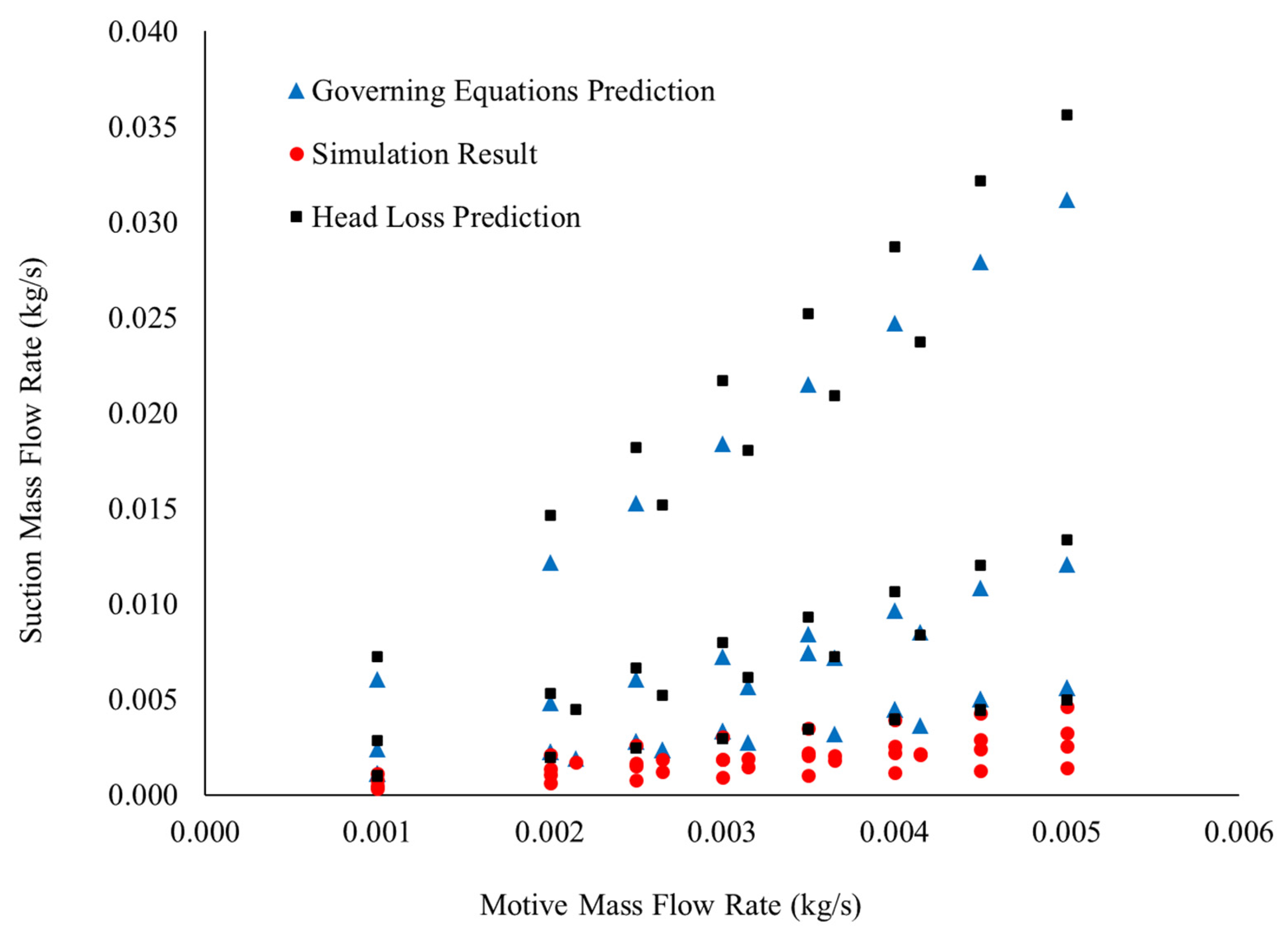
Despite the relative simplicity of the Venturi nozzle and how well known the Venturi effect is, it is not straightforward to calculate the suction flow rate of these nozzles. The Bernoulli equation can be used to determine velocity from a known pressure drop but is not applicable to these nozzles because of the mixing of the motive and suction streams. Gas dynamics relationships could be used to determine the low pressure at the throat of the nozzle based on the Mach number, but the Bernoulli equation or Darcy–Weisbach equation, which do not account for mixing, would still be needed to determine the suction flow rate from the calculated pressure difference. Alternatively, energy head loss calculations could be used to determine the outlet flow rate, and therefore the suction flow rate, based on a known pressure drop and major and minor losses across the entire nozzle; however, charts and empirical equations for the friction factor are based on constant cross section pipes or ducts and it is therefore difficult to accurately determine for nozzles with variable cross sections. Sample calculations for using governing equations and head loss to determine the suction flow rate were performed and are presented in Section 3.
In this paper, we present an empirical model or correlation that can be used as a design guide for low-pressure, subsonic Venturi nozzles for cases of air and air mixing, as well as air and steam mixing. Low-pressure, subsonic Venturi nozzles without diffusers were investigated experimentally, analytically, and numerically. The results of these investigations are combined into empirical models for the suction ratio as a function of the dimensionless groups formed from the geometric parameters, operating conditions, and fluid properties. The empirical model for suction ratio can be used to inform the design of Venturi nozzles given a desired suction ratio. This work allows one to determine the suction ratio of a Venturi nozzle based on known geometry and operating conditions.

2. Simulation and Experimental Validation Methodology

Fifteen different Venturi nozzles were designed and simulated in ANSYS Fluent [38] to determine the effect of the geometry and operating conditions on the suction flow rate, with a total of 109 case studies considered. The geometries were simulated with different suction inlet pressures and motive mass flow inlet boundary conditions. In all cases, it was assumed that the outlet of the nozzle was at ambient pressure. The simulations were experimentally validated by measuring the pressure drop in the nozzles from the motive inlet to the outlet as a function of the motive mass flow rate and geometry. The results of those experiments were used to validate the simulations of the nozzles. In this study, the motive stream was air and the suction stream was either air or steam. The experimental setups and simulations are described in the following sections.

2.1. Air Mixing Experiment

In order to determine the mass flow rate suctioned into a nozzle by the Venturi effect, several Venturi mixing nozzles were designed in SolidWorks© and 3D printed on a MakerBot Replicator+, using CPE+ material. Figure 1 shows the internal geometry of one Venturi mixing nozzle. All geometries considered have the same basic shape as shown in Figure 1, with different motive diameters, throat diameters, suction inlet diameters, and mixing lengths.
The goal of these experiments was to determine the pressure drop across different Venturi nozzles as the motive mass flow rate was varied and to use the measured pressure drop to validate CFD simulations used to determine model boundary flow conditions. To achieve this goal, an experimental setup, shown in Figure 2, was developed. The air mass flow rate into the motive inlet of the nozzle was controlled using a pressure regulator (1) and measured using an Endress + Hauser Promass I Coriolis flow meter, with an instrument uncertainty of ±0.5% of the reading (2). The motive mass flow rate was varied from 1 g/s to 5 g/s. The outlet of the nozzle was open to ambient pressure. This experiment was conducted with two different suction inlet conditions. The first was with the suction inlet open to ambient and the second was with the suction inlet sealed such that there could be no flow into the nozzle from the suction inlet. The motive pressure drop (dP) across the nozzle (3) was measured for both cases using a Setra 230 differential pressure transducer with a full scale of 1 psi and an instrument uncertainty of ±0.25% of full scale or 14 Pa.
The motive pressure drop was used as a proxy measurement for the suction flow rate because when a flow meter was attached to either the suction inlet or outlet of the nozzle to directly measure the suction flow rate, a pressure drop was introduced in the system such that there was no suction flow. There were 36 experimental data points without suction and 36 data points with suction for the air and air mixing experiment. Table 1 shows the nozzles and motive mass flow rates tested for each nozzle. Each experiment was repeated three times.

2.2. Air and Steam Mixing Experiment

In order to determine the suction flow rate with steam as the suction fluid, a similar procedure was used to measure the motive pressure drop as a proxy measurement for the suction flow rate because a direct measurement of the suction flow rate adds an additional pressure drop on the suction side and changes the suction flow rate. The experimental design is shown in Figure 3. The setup is similar to the previous experimental design, but with a few additional components. To supply air flow to the motive inlet, air was fed through a pressure regulator (1), into a Endress + Hauser Promass I Coriolis flow meter (2) and then an Omega AHPF-121 inline heater (4) that was controlled by an ITC-100VH PID (3). The pressure regulator (1) was adjusted until the desired air motive flow rate was read on the Coriolis flow meter (2). This allowed the mass flow rate of air to be measured, and the temperature of the air to be increased just before entering the nozzle to minimize condensation in the nozzle. An industrial 12 kW SteamSpa steam generator (9) was used to supply steam to the suction inlet. The steam generator produces a single source of steam, which is then split into two hoses (7 and 8) upon leaving the generator. The first of these hoses (7) was connected to the suction inlet of the nozzle (6), while the second (8) was directed away from the experimental setup to serve as a bypass for the steam not entering the nozzle. The opening of the second hose (8) was restricted using a clamp so that constant pressure could be maintained at the suction inlet as the motive flow varied between experiments.
Instrumentation locations can be seen in Figure 3, represented by dP for the motive pressure drop, P for the gage static suction pressure, and T for the thermocouple at the motive inlet to measure the air temperature. One Setra 230 differential pressure transducer with a full scale of 5 psi was used to measure the motive pressure drop from the motive inlet to the outlet. A second Setra 230 differential pressure transducer with a full scale of 1 psi was connected to the steam inlet, with the other side open to ambient, to read the gage static pressure at that location. Air temperature was held constant at 105 °C to ensure it was above the saturation temperature of the steam to avoid phase change in the nozzle. Air mass flowrates were varied between 1.5 and 4.5 g/s. The T1 and T3 nozzles were tested, the geometric details of these nozzles are shown in Table 1, with a total of 11 data points. Each test was repeated three times.
For these experiments, the sources of uncertainty were the Coriolis flow meter, the differential pressure transducers, and the thermocouple. The mass flow rate was measured using an Endress + Hauser Promass I Coriolis flow meter with an instrument uncertainty of ±0.5% of the reading. The suction inlet pressure (9) was measured using a Setra 230 differential pressure transducer with a full scale of 1 psi and an instrument uncertainty of ±0.25% of full scale or 14 Pa. The motive inlet pressure drop (10) was measured using a Setra 230 differential pressure transducer with a full scale of 5 psi and an instrument uncertainty of ±0.25% of full scale or 70 Pa. The type k thermocouple used to measure the air temperature had an instrument uncertainty of ±2.2 °C.

2.3. Air Mixing Determination and Validation

CFD simulations were used as a tool to determine the suction flow rate from the measured pressure drop, such that the simulations, once validated, could provide the basis for the empirical model development. ANSYS Fluent 19.2 [38] was used for all CFD simulations. The geometries and boundary conditions from the experiment were used to determine the suction mass flow rate for each experimental case.
For each simulation case, the motive flow rate, motive pressure drop across the nozzle, and static pressure at the suction inlet were known from the experiments. For the case with no suction, the suction inlet was defined as a wall rather than an inlet in simulation so no flow could cross the boundary. For the case with suction, the suction inlet was open to ambient conditions and thus the suction inlet gage static pressure was set to zero. The motive inlet was defined as a mass flow inlet boundary. The nozzle outlet was to open ambient conditions in all cases, so the outlet boundary condition was defined to be zero gage static pressure. The energy model and realizable k-ε turbulence model were the only models used. The simulations were steady, to mimic the steady state measurements of the experiments. A pressure-based solver with a second-order discretization scheme was used for each simulation. The SIMPLE pressure-velocity coupling algorithm was also used for each simulation. Additionally, the ambient pressure condition was set to match the ambient pressure of the experiments (88 kPa). Each simulation was considered to be converged when all residuals had values less than 0.0001 for air mixing and 0.001 for air and steam mixing. The measured motive pressure drop from experiments was compared to the simulated motive pressure drop from CFD to validate each simulation. Three nozzles were tested for each suction condition.
Symmetry was used so only half of the fluid body (Figure 1) was meshed and simulated. In the simulations, the symmetrical half of the nozzle fluid body was meshed, using a 3D linear mesh, and mesh size was reduced (increasing resolution) until residuals were less than 0.0001 and the predicted suction mass flow rate varied by less than 0.2% from one mesh to the next, indicating that the primary result of interest from the simulation was independent of the mesh. The results of the mesh independence study are shown in Figure 4. Table 2 shows the grid refinement study and discretization error with a fine-grid convergence index ( C G I f i n e 21 ) of 5.5% and 0.7% for two critical parameters [39].
Figure 5 and Figure 6 show the experimental results for the closed and open suction inlet, respectively, for each tested nozzle compared to the simulation result. For all motive flow rates and suction conditions, the experimental and simulated results for motive mass flow rate agree to within ±10%. The no suction case has a mean absolute percentage error of 7.5% and a root mean square error of 8.4%. The suction case has a mean absolute percentage error of 5.7% and a root mean square error of 6.5%. The error was calculated as the difference between the experimental and simulated pressure drop. Based on the ±10% agreement between the simulation and experiments, the simulations were considered to be validated. From the validated simulation, the suction mass flow rate can be found.

2.4. Air and Steam Mixing Determination and Validation

For the steam simulation validation, the same procedure was followed as described above for air mixing. For the case of steam mixing, the suction inlet was at a pressure above ambient due to steam entering the nozzle at that location. For these simulations the multi-species model was used with ideal gas air and steam. With the exception of changing the suction inlet boundary condition to be steam above ambient pressure and using the Fluent multi-species model, all other boundary conditions, meshes, and models were the same as for the air mixing tests. The simulations were considered to be converged when the residuals reached 0.001. As shown in Figure 7, the experimental and simulation results agree within ±11%, with a mean absolute error of 10.5% and a root mean square error of 10.6% for each steam mixing case, and therefore the simulation is considered to be validated. For all cases, the experimental data had a lower motive pressure drop than the simulation predicted. This could be due to the fact that phase change was neglected in the simulations, but there was a small amount of condensation in the nozzle during each experiment.
In summary, both the air mixing as well as the air and steam mixing cases are validated with a maximum error of 10.6%, and therefore the simulations were considered to be validated and trusted moving forward with a parametric study and correlation development.

3. Governing Equations and Flow Head Calculations

As previously discussed, some applications, such as water treatment, require precise knowledge of the suction flow rate, or suction ratio, in order to successfully operate. Unfortunately, the suction ratio of the nozzles can be difficult to accurately determine using flow design calculations. As an example, here governing equation calculations and energy head loss calculations are used to calculate the suction flow rate and compared to the suction flow rate from the validated simulations [40].
The governing equation calculation approach was evaluated based on the continuity (Equation (1)), conservation of energy (Equation (2)), and conservation of momentum (Equation (3)) equations. For this analysis, a control volume that crosses the throat, suction inlet, and outlet of each nozzle was considered. For air and air mixing, Equation (6) was used to determine the enthalpy of the outlet stream. For air and steam mixing, where the psychrometrics of the humid air must be considered, Equations (6)–(9) were used to determine the relative humidity and thus the enthalpy of the outlet humid stream. For both cases, Equations (4) and (5) were used to determine the densities of the air at the throat and outlet stream. Alternatively, a flow head loss method based on the head form of the energy equation could be used to calculate the suction mass flow rate based on the major and minor losses in each nozzle; however, it was found that the head loss method is less accurate than the governing equation approach, as shown in Figure 8.
Figure 8 shows the suction mass flow rate as determined by the governing equations and validated simulations versus the motive mass flow rate for each experimental data point. On average, the governing equations predict the suction mass flow rate with a 270% error. This method is insufficiently accurate to determine the suction mass flow rate of the low-pressure Venturi nozzles considered in this study. A different method is necessary to precisely calculate the suction mass flow rate of these nozzles, and thus inform the design of the nozzles. The empirical models presented in Section 5 of this paper allow for precise calculation of the suction ratio and therefore suction mass flow rate.
m ˙ m o t i v e + m ˙ s u c t i o n = m ˙ o u t l e t
m ˙ m o t i v e ( h t h r o a t + 1 2 V t h r o a t 2 ) + m ˙ s u c t i o n ( h s u c t i o n + 1 2 V s u c t i o n 2 ) = ( m ˙ o u t l e t ) ( h o u t l e t + 1 2 V o u t l e t 2 )
P t h r o a t g a g e A m o t i v e = m ˙ o u t l e t V o u t l e t m ˙ m o t i v e V t h r o a t m ˙ s u c t i o n V s u c t i o n
ρ t h r o a t = f ( P t h r o a t ,   T a m b i e n t )
ρ o u t l e t = m ˙ m o t i v e ρ t h r o a t + m ˙ s u c t i o n ρ s u c t i o n m ˙ m o t i v e + m ˙ s u c t i o n
h o u t l e t a i r = f ( ρ o u t l e t , P o u t l e t )
h o u t l e t s t e a m = f ( T o u t l e t , P o u t l e t )
ω = m ˙ s u c t i o n s t e a m m ˙ m o t i v e
h o u t l e t = h o u t l e t a i r + ω h o u t l e t s t e a m

4. Parametric Study

In order to determine the suction mass flow rate for different nozzles, a parametric study was completed in using the validated CFD simulations. Fifteen different geometries with varying motive inlet diameters, throat diameters, suction inlet diameters, and mixing lengths were simulated with varying boundary conditions. All geometries are given in Table 3. Geometries were chosen to provide a range of values for each of the selected geometrical parameters: motive diameter, throat diameter, suction diameter, and mixing length. Each parameter was varied to provide at least four different values. These values were chosen such that the average of each geometric parameter provides a fixed suction ratio to keep the ratio of steam to air below the carrying capacity of water in air for the majority of steam mixing cases. It was confirmed that flow in each geometry remains subsonic and incompressible for all relevant conditions prior to including the geometry in the parametric study.
All flow conditions are shown in the simulation test matrix in Table 4. The motive inlet was defined to be a mass flow inlet with a flow rate of either 5.2 or 20.8 g/s. These flow rates were chosen because 20.8 g/s is the desired flow rate for one application of these nozzles and 5.2 g/s was selected to provide a lower range of suction ratios [33]. The motive inlet fluid was ideal gas air for all cases. The suction inlet boundary condition was a pressure inlet with a static gage pressure of either 10 Pa, 100 Pa, or 500 Pa. The suction fluid was either ideal gas air or steam. For all cases, the nozzle outlet boundary condition was defined to be 0 Pa gage. Every combination of geometry and boundary conditions summed to 109 different cases considered in the parametric study. For each case, the suction mass flow rate and dimensionless suction ratio, or ratio of suction mass flow rate to motive mass flow rate, were calculated.

Empirical Model Formulation

In order to develop a model for the suction ratio as a function of the geometry and operating conditions, the form of the model must first be determined. The suction mass flow rate ( m s ˙ ) was taken to be a function of the motive mass flow rate ( m ˙ m ), the motive inlet area ( A m ), the throat diameter ( D t ), the suction inlet diameter ( D s ), the mixing length ( L ), the motive fluid density ( ρ m ), the suction fluid kinematic viscosity ( ν s ), the motive fluid viscosity ( μ m ), and the gage static pressure at the suction inlet ( P s t a t i c ) (Equation (10)). Consequently, the functional form for the suction mass flow rate becomes:
m s ˙ = f ( m ˙ m ,   A m , D t ,   D s ,   L ,   ρ m ,   ν s ,   μ m ,   P s t a t i c )
The Buckingham Pi Theorem was used to determine the dimensionless groups that define this system as:
m ˙ s m ˙ m = [ ( A m A t ) a ( L D s ) b ( m ˙ m   μ m   D t ) c ( ν s ν m ) d ( P s t a t i c   D t 4   ρ m   π 2   8   m m ˙ 2 ) e ]
The third independent dimensionless group on the right side of the above expression ( m ˙ m   μ m   D t ) is the Reynolds number at the throat of the nozzle. The last independent dimensionless group ( P s t a t i c   D t 4   ρ m   π 2   8   m m ˙ 2 ) is the ratio of the gage static pressure at the suction inlet to the dynamic pressure at the throat. Using these definitions, Equation (11) can be written as:
m s ˙ m ˙ m = [ ( A m A t ) a ( L D s ) b ( R e m o t i v e ,   t h r o a t ) c ( ν s ν m ) d ( P s t a t i c ,   s u c t i o n P d y n a m i c ,   t h r o a t ) e ]
The coefficient and exponents of the correlation were determined using a multi-variable global optimization code in Python. The global constrained minimization algorithm determined the best fit for the coefficient and exponents of the correlation based on the 109 parametric study cases, using the Levenberg–Marquardt scheme [41,42].

5. Results

Seven different empirical models were developed and evaluated to determine which parameters are most important to prediction of nozzle performance, and to find which empirical model is best able to predict the nozzle performance. Details of each empirical model are given below. Every empirical model considered, as well as their errors and ranges of applicability are summarized in Table 5 in order to provide a design reference for Venturi nozzles.

5.1. Suction Ratio Models

Comparing the suction ratio predicted by the empirical model (Equation (17) in 
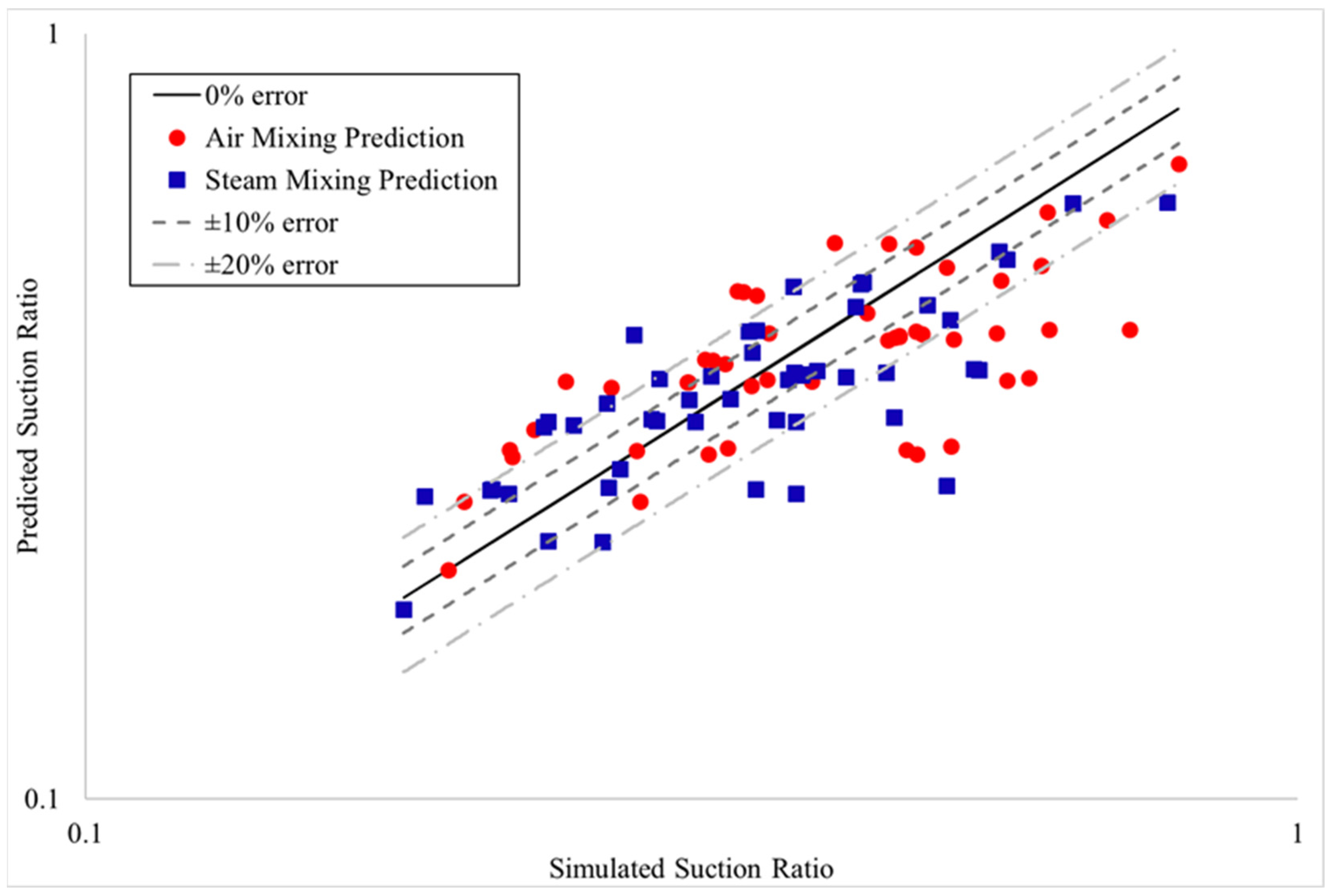
Table 5) to the suction ratio determined using the validated simulations, the empirical model predicts the suction ratio with a mean absolute percentage error of 22% and a root mean square error of 27%. Figure 9 shows the suction ratio predicted by the global correlation compared to the suction ratio determined by the validated simulations. In Figure 9, the red circles indicate the correlation prediction for air mixing cases and the blue squares indicate the prediction for steam mixing. The solid black line indicates what the suction ratio should be to have 0% error with the simulated suction ratio, and the dashed lines show ±10% and ±20% of the simulated value. Both air mixing and steam mixing cases are equally well predicted by the global correlation. If the correlation is developed considering only the air mixing cases (Equation (18)) or only considering the air and steam mixing cases (Equation (19)), the correlation becomes slightly more accurate but not significantly so, as shown in Table 5. Instead, the error in the global correlation comes from two flow regimes being predicted by the same correlation; there is a clear discrepancy in Figure 9 at the simulated suction ratio of one. Cases with low suction ratios, less than one, are relatively well predicted with a mean absolute percentage error of 20% while cases with high suction ratios, greater than one, are relatively poorly predicted with a mean absolute percentage error of 43%.
The increase in mean absolute percentage error for the high suction ratio cases indicates that the correlation does not well predict the behavior of the mixing nozzles for those cases. Each of the high suction ratio cases has a low Reynolds number and a high-pressure ratio. This indicates that the high suction ratio cases may be driven more by the applied static pressure at the suction inlet than the Venturi effect from the motive mass flow rate and throat diameter. Additionally, the low suction ratio cases all have a relatively high Reynolds number and a relatively low pressure ratio. If the low and high suction ratio cases are considered to be driven by different phenomena, inertia and pressure, respectively, then it may be better to model each regime separately.
If only the low suction ratio cases are considered in the optimization, the result is Equation (20), given in Table 5. The low suction ratio correlation predicts the suction ratio with a mean absolute percentage error of 18%, and a root mean square error of 22% as shown in Figure 10.
If only the high suction ratio cases are considered in the optimization, the result is Equation (21). The high suction ratio correlation predicts the suction ratio with a mean absolute percentage error of 5%, and a root mean square error of 6%, as shown in Figure 11. Separating the global correlation including both high and low suction ratios into one correlation for low suction ratio and one correlation for high suction ratio allows for more accurately informed decisions about the design of a Venturi nozzle geometry, assuming that the desired suction ratio can be identified as either high or low. Figure 12 shows the suction ratio predicted by the low and high suction ratios on one plot, with the correlation used for each suction ratio range.
A sensitivity analysis was conducted by increasing then decreasing the value of each dimensionless group by 10% compared to the original value and calculating the maximum relative error, mean absolute percentage error, and root mean square error for each case. The sensitivity analysis revealed that the area ratio ( A m A t ) had the largest impact on the error of each correlation of all the dimensionless groups, followed by the kinematic viscosity ratio ( ν s ν m ) and then the Reynolds number ( m ˙ m   μ m   D t ) . Comparing the effect of each dimensionless group between the low and high suction ratio cases, it was found that the geometry has a larger impact on the suction ratio for the low suction ratio cases than the high suction ratio cases. The high suction ratio cases are more dependent on operating conditions than the geometry of the nozzle. These results support the hypothesis that the suction flow for high suction ratio cases is largely driven by the applied static pressure at the suction inlet, while the low suction ratio cases are more dependent on geometry because they are truly Venturi driven flow and the area ratio is critical to the performance.

5.2. Momentum Ratio and Dynamic Pressure Ratio Models

Given the apparent dependence of the global suction ratio correlation on pressure, two alternative empirical models were evaluated: momentum ratio and dynamic pressure ratio. For these models, either the momentum ratio or the dynamic pressure ratio is predicted by the global correlation, instead of the suction ratio. For each of these cases, the form of the correlation can be determined, again, using the Buckingham Pi Theorem.
For the momentum ratio, the suction momentum term ( ρ s m ˙ s ) was considered to be a function of the motive mass flow rate ( m ˙ m ), the motive inlet area ( A m ), the throat diameter ( D t ), the suction inlet diameter ( D s ), the mixing length ( L ), the motive fluid density ( ρ m ), the motive fluid viscosity ( μ m ), and the gage static pressure at the suction inlet ( P s t a t i c ), which, when non-dimensionalized, yields the following:
ρ s m ˙ s = f ( m ˙ m ,   A m ,   D t ,   L ,   D s ,   μ m ,   ρ m ,   ν s ,   P s t a t i c )  
ρ s   m s ˙ ρ m m m ˙ = [ ( A m A t ) a ( L D s ) b (   m m ˙   μ m   D t ) c ( ν s ν m ) d ( P s t a t i c   D t 4   ρ m   π 2   8   m m ˙ 2 ) e ]
When the momentum ratio correlation is optimized, it yields Equation (22), also given in Table 5. The resulting correlation yields a mean absolute percentage error of 28%, and a root mean square error of 36% when compared to the validated simulations.
For the dynamic pressure ratio, the suction dynamic pressure ( 8   m m ˙ 2 /( D t 4 ρ s π 2 )) was considered to be a function of the motive mass flow rate ( m ˙ m ), the motive inlet area ( A m ), the throat diameter ( D t ), the mixing length ( L ), the motive fluid density ( ρ m ), the motive fluid viscosity ( μ m ), and the gage static pressure at the suction inlet ( P s t a t i c ), yielding Equation (15) below, which when non-dimensionalized gives Equation (16). The coefficient and exponents determined using the global optimization are shown in Equation (23). The global dynamic pressure ratio has a mean absolute percentage error of 48%, and a root mean square error of 56%. In Equation (16), the mixing length is nondimensionalized using the throat diameter, rather than the suction inlet diameter as in the suction ratio and momentum ratio models because the suction diameter is on the independent side of the equation, but the remaining terms are identical to those of the previously discussed correlations.
8 m ˙ s D S 4 ρ s π 2 = f ( m ˙ m ,   A m ,   D t ,   L ,   μ m ,   ρ m ,   ν s , P s t a t i c )
m ˙ s D t 4 ρ m m ˙ m D s 4 ρ s = [ ( A m A t ) a ( L D t ) b (   m ˙ m   μ m D t ) c ( ν s ν m ) d ( P s t a t i c   D t 4   ρ m   π 2 8   m ˙ m 2 ) e ]
Table 5. Summary of proposed empirical models, ranges of applicability, mean absolute percentage error (MAPE), and root mean square error (RSME).
Empirical ModelMAPERSMEApplicabilityEquation
Global suction ratio m ˙ s m ˙ m = 3.88 [ ( A m A t ) 0.734 ( L D s ) 0.006 ( m ˙ m   μ m D t ) 0.288 ( ν s ν m ) 2.17 ( P s t a t i c   D t 4   ρ m   π 2 8   m ˙ m 2 ) 0.123 ] 22%27% 0.183   m s ˙ m m ˙ 2.294 (17)
20,690   R e t 165,521
0.0001 P s t a t i c P d y n a m i c 1.319
Air mixing, air and steam mixing
Air only suction ratio m ˙ s m ˙ m = 12.7 [ ( A m A t ) 0.785 ( L D s ) 0.134   ( m ˙ m   μ m D t ) 0.396 ( P s t a t i c   D t 4   ρ m   π 2 8   m ˙ m 2 ) 0.12 ] 22%26% 0.199   m s ˙ m m ˙ 2.294 (18)
20,690   R e t 165,521
0.0001 P s t a t i c P d y n a m i c 1.319
Air mixing
Steam only suction ratio m ˙ s m ˙ m = 1.5 [ ( A m A t ) 0.688 ( L D s ) 0.147 (   m ˙ m   μ m D t ) 0.214 ( P s t a t i c   D t 4   ρ m   π 2 8   m ˙ m 2 ) 0.124 ] 20%25% 0.183   m s ˙ m m ˙ 1.787 (19)
20,690   R e t 165,521
0.0001 P s t a t i c P d y n a m i c 1.319
Air and steam mixing
Low suction ratio
(suction ratio less than one)
m ˙ s m ˙ m = 0.385 [ ( A m A t ) 0.594 ( L D s ) 0.03 (   m ˙ m   μ m D t ) 0.075 ( ν s ν m ) 1.782 ( P s t a t i c   D t 4   ρ m   π 2 8   m ˙ m 2 ) 0.09 ] 18%22% 0.183   m s ˙ m m ˙ 0.797 (20)
20,690   R e t 165,521
0.0001 P s t a t i c P d y n a m i c 0.0825
Air mixing, air and steam mixing
High suction ratio
(suction ratio greater than one)
m ˙ s m ˙ m = 1.79 [ ( A m A t ) 0.624 ( L D s ) 0.271 ( m ˙ m   μ m D t ) 0.138 ( ν s ν m ) 3.127 ( P s t a t i c   D t 4   ρ m   π 2 8   m ˙ m 2 ) 0.166 ] 5%6% 1.157   m s ˙ m m ˙ 2.294 (21)
20,690   R e t 41,380
0.00165 P s t a t i c P d y n a m i c 1.319
Air mixing, air and steam mixing
Momentum Ratio ρ s m ˙ s ρ m m ˙ m = 3.88 [ ( A m A t ) 0.734 ( L D s ) 0.006 (   m ˙ m   μ m D t ) 0.288 ( ν s ν m ) 3.17 ( P s t a t i c   D t 4   ρ m   π 2 8   m ˙ m 2 ) 0.123 ] 28%36% 0.115   ρ s   m s ˙ ρ m m m ˙ 2.294 (22)
20,690   R e t 165,521
0.0001 P s t a t i c P d y n a m i c 1.319
Air mixing, air and steam mixing
Dynamic pressure ratio m ˙ s D t 4 ρ m m ˙ m D s 4 ρ s = 8.58 [ ( A m A t ) 0.626 ( L D t ) 1.121 (   m ˙ m   μ m D t ) 0.407 ( ν s ν m ) 0.081 ( P s t a t i c   D t 4   ρ m   π 2 8   m ˙ m 2 ) 0.364 ] 48%56% 0.00250   m s ˙ 2 D t 4 ρ m m m ˙ 2 D s 4 ρ s 3.130 (23)
20,690   R e t 165,521
0.0001 P s t a t i c P d y n a m i c 1.319
Air mixing, air and steam mixing

5.3. Venturi Nozzle Design Guide

Based on the results presented in Section 5.2, the suction ratio models (Equations (17)–(23)) can be used to determine the flow rate of a suction fluid into a low-pressure, subsonic Venturi nozzle. There are many commercially available Venturi nozzles [43,44,45,46]; however, for subsonic nozzles, it can be difficult to determine which nozzle to select or what suction flow rate to expect from a particular nozzle.
If a particular suction ratio is desired for an application of a subsonic, low-pressure Venturi nozzle, one could find several commercially available nozzle options and plug those geometries into the suction ratio empirical models from Section 5.2, along with some operating conditions from the application, and find the geometry that is best suited to deliver the desired suction ratio. Additionally, one could use the empirical models to design a geometry that is ensured to deliver the desired suction ratio, rather than using a commercially available option.
As an example, for a humidification–dehumidification water treatment system, a specific suction ratio of 0.33 may be desired to ensure a maximum amount of water is treated without oversaturating the holding capacity of the air. Given this known suction ratio, the other parameters in the empirical model can be adjusted to inform the design of the nozzle. It is assumed that the ratio of kinematic viscosities is known, and therefore the adjustable dimensionless groups are the area ratio, length ratio, Reynolds number, and pressure ratio. To begin, choose an assumed throat diameter as the throat diameter appears in three of the five dimensionless groups in the suction ratio empirical correlation. Once the throat diameter has been assumed, select a motive mass flow rate. The motive mass flow rate can be calculated if there is a desired velocity in the system after the nozzle, otherwise an approximate value may be assumed. Based on these two selected parameters, the Reynolds number is known as well as the dynamic pressure at the throat of the nozzle. Next, the static pressure at the suction inlet can be determined so the pressure ratio may be fully defined. The static pressure at the suction inlet may be easily defined if the suction inlet is open to ambient pressure. In the case of the humidification–dehumidification example, the pressure is expected to be slightly above ambient pressure as steam is generated in a closed system with the suction inlet being the only opening. Once the Reynold number and pressure ratio terms have been defined, the remaining terms are only a function of geometry. Next, the motive area can be defined as the area ratio is more impactful than the length ratio. Finally, the length ratio can be defined. This term may be determined by other constraints such as a given suction inlet diameter necessary to connect to another component or a given mixing length to ensure the mixed fluids exit the nozzle at a certain location. Based on these assumptions, an approximate suction ratio can be determined from the empirical models and each parameter adjusted iteratively until the desired suction ratio is achieved. As discussed in Section 3, using a head loss calculation to estimate of the suction ratio would yield a suction ratio much too high. Therefore, use of the correlations developed here and presented in Table 5 is recommended for design of low-pressure, subsonic Venturi nozzles.

6. Conclusions

A study on the effect of geometry and operating conditions on the suction ratio of low-pressure, subsonic Venturi mixing nozzles was conducted. An ANSYS CFD model of the Venturi nozzle mixing was experimentally validated, and then used to calculated nozzle performance over a wide range of geometries and operating conditions. Governing equation calculations and flow head calculations were also used to determine the suction ratio of the experimentally tested nozzles and was found to be very inaccurate in these cases. To determine the suction ratio more accurately, seven potential empirical models were developed to examine the effect of different thermophysical parameters on the suction ratio and identify the parameters most critical to accurate prediction. The foundation for each of the empirical models is the results of a parametric study of nozzle geometry and operating conditions.
The empirical models for suction ratio are more accurate than the empirical models for either momentum ratio or dynamic pressure ratio. For the five suction ratio models developed, the average mean absolute percentage error is 17%. Separating the flow into high-suction ratio and low-suction ratio regimes had the largest impact on the error of the models indicating that the regime change is the most critical aspect of nozzle operation. Based on these results, any of the presented suction ratio empirical models (global, air only, air and steam mixing only, high-suction ratio, or low-suction ratio) can be used to determine the suction ratio of a low-pressure, subsonic Venturi nozzle within 22%, or a more specific model may be used if the application of the nozzle (low-suction ratio, air only mixing, etc.) with reduced error.
This work can be used to inform the design of low-pressure, subsonic Venturi nozzles for many applications. The suction ratio empirical models are, on average, 34-foldmore accurate than the flow head loss approach. The suction ratio empirical models can be used to determine the suction ratio or nozzle design when precise mixing is required for a given application.
While the correlations proposed in this study provide a good initial design, it will be advantageous to have a secondary tool for a more accurate nozzle design. To that end, these correlations can be used as the basis for physics-guided machine learning algorithms to serve as a more accurate secondary tool for detailed nozzle design and analysis. The authors are in the process of developing such a design tool. The results will be evaluated and published in a follow-up article.

Author Contributions

Conceptualization, H.O., J.L. and B.A.; methodology, H.O., T.M., and X.Z.; software, H.O. and X.Z.; validation, H.O.; formal analysis, H.O.; writing—original draft preparation, H.O. and T.M.; writing—review and editing, H.O., B.A. and J.L.; supervision, B.A.; funding acquisition, B.A. All authors have read and agreed to the published version of the manuscript.

Funding

This research was funded by US Department of Energy, Advanced Research Projects Agency—Energy (ARPA-E) award number DE-AR-0001000.

Institutional Review Board Statement

Not applicable.

Informed Consent Statement

Not applicable.

Data Availability Statement

Not applicable.

Acknowledgments

The authors thank ARPA-E for their support of this research.

Conflicts of Interest

The authors declare no conflict of interest.

References

  1. Ariafar, K. Performance evaluation of a model thermocompressor using computational fluid dynamics. Int. J. Mech. 2012, 6, 35–42. [Google Scholar]
  2. Meakhail, T.A.; Zien, Y.; Elsallak, M.; Abdelhady, S. Experimental study of the effect of some geometric variables and number of nozzles on the performance of a subsonic air—Air ejector. Proc. Inst. Mech. Eng. 2008, 222, 809–818. [Google Scholar] [CrossRef]
  3. Manzano, J.; Palau, C.V.; Moreira de Azevedo, B.; do Bomfim, G.V.; Vasconcelos, D.V. Characterization and selection method of Venturi injectors for pressurized irrigation. Rev. Ciência Agronômica 2018, 49, 201–210. [Google Scholar] [CrossRef]
  4. Bilalis, D.; Karkanis, A.; Savvas, D.; Kontopoulou, C.-K.; Efthimiadou, A. Effects of fertilization and salinity on weed flora in common bean (‘Phaseolus vulgaris’ L.) grown following organic or conventional cultural practices. Aust. J. Crop Sci. 2014, 8, 178–182. [Google Scholar]
  5. Okzan, F.; Ozturk, M.; Baylar, A. Experimental investigations of air and liquid injection by venturi tubes. Water Environ. J. 2006, 20, 114–122. [Google Scholar]
  6. Little, A.B.; Garimella, S. A critical review linking ejector flow phenomena with component- and system-level performance. Int. J. Refrig. 2016, 70, 243–268. [Google Scholar] [CrossRef]
  7. Little, A.B.; Bartosiewicz, Y.; Garimella, S. Visualization and validation of ejector flow field with computational and first-principal analysis. J. Fluids Eng. 2015, 137, 1107. [Google Scholar] [CrossRef]
  8. Lin, C.; Cai, W.; Li, Y.; Hu, Y.; Giridharan, K. Numerical investigation of geometry parameters for pressure recovery of an adjustable ejector in multi-evaporator refrigeration system. Appl. Therm. Eng. 2013, 61, 649–656. [Google Scholar] [CrossRef]
  9. Varga, S.; Oliveira, A.C.; Ma, X.; Omer, S.A.; Zhang, W.; Riffat, S.B. Experimental and numerical analysis of a variable area ratio steam ejector. Int. J. Refrig. 2011, 34, 1668–1675. [Google Scholar] [CrossRef]
  10. Sun, D.-W. Variable geometry ejectors and their applications in ejector refrigeration systems. Energy 1996, 10, 919–929. [Google Scholar] [CrossRef]
  11. Huang, B.J.; Hu, S.S.; Le, S.H. Development of an ejector cooling system with thermal pumping effect. Int. J. Refrig. 2006, 29, 476–484. [Google Scholar] [CrossRef]
  12. Li, X.; Wang, T.; Day, B. Numerical analysis of the performance of a thermal ejector is a steam evaporator. Appl. Therm. Eng. 2010, 30, 2708–2717. [Google Scholar] [CrossRef]
  13. Bora, B.J.; Debnath, B.K.; Gupta, N.; Saha, U.K.; Sahoo, N. Investigation on the flow behaviour of a venturi type gas mixer designed for dual fuel diesel engines. Int. J. Emerg. Technol. Adv. Eng. 2013, 3, 202–209. [Google Scholar]
  14. Papadakis, E.; Raptopoulos, F.; Koskinopoulou, M.; Maniadakis, M. On the use of vacuum technology for applied robotic systems. In Proceedings of the 2020 6th International Conference on Mechatronics and Robotics Engineering (ICMRE), Barcelona, Spain, 12–15 February 2020; pp. 73–77. [Google Scholar]
  15. Rodrigues, A.; Camargo, E.; Ciolfi, M. Venturi Tube Application to Improve the Vacuum Assistance for Brake Systems; SAE International: Warrendale, PA, USA, 2013. [Google Scholar]
  16. Xu, J.; Liu, X.; Pang, M. Numerical and experimental studies on transport properties of powder ejector based on double venturi effect. Vacuum 2016, 134, 92–98. [Google Scholar] [CrossRef]
  17. Kroll, E.A. The design of jet pumps. Chem. Eng. Prog. 1947, 1, 21–24. [Google Scholar]
  18. Eames, I.W. A new prescription for the design of supersonic jet pumps: The constant rate of momentum change method. Appl. Therm. Eng. 2002, 22, 121–131. [Google Scholar] [CrossRef]
  19. Hoggarth, M.L. The design and performance of high-pressure injectors and gas jet boosters. Proc. Inst. Mech. Eng. 1970, 185, 755–766. [Google Scholar] [CrossRef]
  20. Munday, J.T.; Bagster, D.F. A new theory applied to steam jet refrigeration. Ind. Eng. Chem. Process Des. Dev. 1997, 16, 442–449. [Google Scholar] [CrossRef]
  21. Riffat, S.B.; Everitt, P. Experimental and CFD modeling of an ejector system for vehicle air conditioning. J. Inst. Energy 1999, 72, 41–47. [Google Scholar]
  22. Bartosiewicz, Y.; Aidoun, Z.; Desevaux, P.; Mercadier, Y. Numerical and experimental investigations on supersonic ejectors. Int. J. Heat Fluid Flow 2005, 1, 56–70. [Google Scholar] [CrossRef]
  23. Fu, W.; Liu, Z.; Li, Y.; Wu, H.; Tang, Y. Numerical study for the influences of primary steam nozzle distance and mixing chamber throat diameter on steam ejector performance. Int. J. Therm. Sci. 2018, 132, 509–516. [Google Scholar] [CrossRef]
  24. Keenan, J.H.; Neumann, E.P. A simple air ejector. ASME J. Appl. Mech. 1942, 62, 75–81. [Google Scholar] [CrossRef]
  25. McGovern, R.K.; Narayan, G.P.; Lienhard V, J.H. Analysis of reversible ejectors and definition of an ejector efficiency. Int. J. Therm. Sci. 2012, 54, 153–166. [Google Scholar] [CrossRef]
  26. Yang, X.; Long, X.; Yao, X. Numerical investigation on the mixing process in a steam ejector with different nozzle structures. Int. J. Therm. Sci. 2012, 56, 95–106. [Google Scholar] [CrossRef]
  27. Ouzzane, M.; Aidoun, Z. Model development and numerical procedure for detailed ejector analysis and design. Appl. Therm. Eng. 2003, 23, 2337–2351. [Google Scholar] [CrossRef]
  28. Shin, D.H.; Gim, Y.; Sohn, D.K.; Ko, H.S. Development of venturi-tube with spiral-shaped fin for water treatment. J. Fluids Eng. 2019, 141, 051303. [Google Scholar] [CrossRef]
  29. Rudolf, P.; Hudec, M.; Stefan, D. Numerical and experimental investigation of the cavitating flow within venturi tube. J. Fluids Eng. 2019, 141, 1101. [Google Scholar]
  30. Frankel, S. Large eddy simulation of turbulent-cavitation interactions in a venturi nozzle. J. Fluids Eng. 2010, 132, 121301. [Google Scholar]
  31. Sundararaj, S.; Selladurai, V. Numerical and experimental study on jet trajectories and mixing behavior of venturi-jet. J. Fluids Eng. 2010, 132, 101104. [Google Scholar] [CrossRef]
  32. Chen, W.; Chong, D.; Yan, J.; Liu, J. The numerical analysis of the effect of geometrical factors on natural gas ejector performance. Appl. Therm. Eng. 2013, 59, 21–29. [Google Scholar] [CrossRef]
  33. Hu, J.; Cao, X.; He, H.; Meng, Z.; Ding, M. Numerical optimization on the geometrical factors of subsonic air-air ejector. In Proceedings of the 9th International Symposium on Symbiotic Nuclear Power Systems for 21st Century, Harbin, China, 9–11 July 2018. [Google Scholar]
  34. Maqsood, A. A study of subsonic air-air ejectors with short bent mixing tubes. Diss. Abstr. Int. 2008, 69, 1911. [Google Scholar]
  35. Vaclav, D. Air to air ejector with various divergent mixing chambers. Appl. Mech. Mater. 2014, 493, 50–55. [Google Scholar]
  36. O’Hern, H.; Nikooei, N.; Zhang, X.; Hagen, C.; AuYeung, N.; Tew, D.; Abbasi, B. Reducing the water intensity of hydraulic fracturing: A review of treatment technologies. Desalin. Water Treat. 2021, 221, 121–138. [Google Scholar] [CrossRef]
  37. Abbasi, B.; Zhang, X.; O’Hern, H.; Nikooei, E. Method and System for Purifying Contaminated Water. U.S. Patent Application No. 16/985,043, 4 August 2020. [Google Scholar]
  38. Ansys Academic Research Fluent, Release 19.2. Ansys, Canonsburg, PA, USA. Available online: https://www.ansys.com/academic (accessed on 18 November 2021).
  39. Celik, I.B.; Ghia, U.; Roache, P.J.; Freitas, C.J. Procedure for estimation and reporting of uncertainty due to discretization in CFD applications. J. Fluids Eng. 2008, 130, 078001. [Google Scholar]
  40. Cengel, Y.A.; Cimbala, J.M. Fluid Mechanics, Fundamentals and Applications; McGraw-Hill: New York City, NY, USA, 2014. [Google Scholar]
  41. Transtrum, M.K.; Sethna, J.P. Improvements to the Levenberg-Marquardt algorithm for nonlinear least-squares minimization. arXiv 2012, arXiv:1201.5885. [Google Scholar]
  42. Elhashimi, M.; Zhang, X.; Abbasi, B. Empirical prediction of saline water atomization pressure loss and spray phase change using local flow pressure analysis. Desalination 2021, 514, 115156. [Google Scholar] [CrossRef]
  43. McMaster-Carr. Available online: https://www.mcmaster.com/venturi/water-aspirator-pumps/ (accessed on 18 November 2021).
  44. McMaster-Carr. Available online: https://www.mcmaster.com/venturi/fixed-flow-air-powered-vacuum-pumps-7/ (accessed on 18 November 2021).
  45. Steel Venturi Style Pneumatic Air Blower. Grainger, Lakeforest, IL, USA. Available online: https://www.grainger.com/product/ALLEGRO-Steel-Venturi-Style-Pneumatic-3TCK2 (accessed on 18 November 2021).
  46. Aluminum Venturi Nozzle For Blow Gun M 12x1.25 (MT). Tameson, Eindhoven, The Netherlands. Available online: https://tameson.com/pneumatics/air-tools/air-nozzles/venturi/aluminum-venturi-nozzle-for-blow-gun-m-12x1p25-mt.html?id_currency=4 (accessed on 18 November 2021).
Figure 1. Cross-section of representative nozzle with key geometric parameters identified.
Applmech 03 00024 g001
Figure 2. Air mixing experimental setup schematic.
Applmech 03 00024 g002
Figure 3. Steam mixing experimental setup schematic.
Applmech 03 00024 g003
Figure 4. Mesh refinement study. Once the number of elements was increased past 828,360, there was effectively no change in the result and mesh independence was reached.
Applmech 03 00024 g004
Figure 5. Motive pressure drop (Pa) vs. motive mass flow rate (g/s) for nozzle tests with no suction. See Table 3 for nozzle geometry details. For the T1 geometry, the uncertainty bars are smaller than the experimental marker used.
Applmech 03 00024 g005
Figure 6. Motive pressure drop (Pa) vs. motive mass flow rate (g/s) for air mixing tests. See Table 3 for nozzle geometry details. For the T1 geometry, the uncertainty bars are smaller than the experimental marker used.
Applmech 03 00024 g006
Figure 7. Motive pressure drop (Pa) vs. motive mass flow rate (g/s) for steam tests. See Table 3 for nozzle geometry details.
Applmech 03 00024 g007
Figure 8. Head loss predicted suction mass flow rate, governing equations predicted suction mass flow rate, and validated simulation suction mass flow rate vs. motive mass flow rate. The suction mass flow rate predicted by the governing equations method is 270% higher than the simulation result. The suction mass flow rate predicted by the head loss method is approximately 380% higher than the mass flow rate from the validated simulation. The simulation has an average error of 8% relative to the experimental data.
Applmech 03 00024 g008
Figure 9. Suction ratio predicted by global suction ratio correlation vs. suction ratio from validated simulation.
Applmech 03 00024 g009
Figure 10. Suction ratio predicted by low suction ratio correlation vs. suction ratio from validated simulation.
Applmech 03 00024 g010
Figure 11. Suction ratio predicted by the high suction ratio correlation vs. the suction ratio from the validated simulation.
Applmech 03 00024 g011
Figure 12. Suction ratio predicted by low and high suction ratio correlations vs. the suction ratio from the validated simulation.
Applmech 03 00024 g012
Table 1. Air mixing experimental test matrix.
Nozzle Name/CodeMotive Diameter (m)Throat Diameter (m)Suction Diameter (m)Mixing Length (m)Motive Mass Flow Rate (g/s)Suction Inlet Condition
T10.040.0120.0270.03851–5Sealed and Open
LR30.040.0160.0270.081–5Sealed and Open
AR50.040.0160.01750.03851–5Sealed and Open
Table 2. Grid refinement study and discretization error.
Grid SpecificationsNumber of Cells: Case I: 4,702,076, Case II: 1,439,997, Case III:828,620 r 21 = 1.48 r 32 = 1.20
Physical Parameter (φ)Suction Mass Flow Rate (kg/s)Motive Pressure Drop (Pa)
φ   i n   Case   I 0.0043258980.95
φ   i n   Case   II 0.0044899020.66
φ   i n   Case   III 0.0046179151.77
φ 2 φ 1 1.64 × 10−439.71
φ 3 φ 2 1.28 × 10−431.11
p 1.591.56
φ e x t 21 0.004148934.04
φ e x t 32 0.004118926.41
e 21 3.8%0.4%
e 32 2.8%0.3%
e e x t 21 4.6%0.5%
e e x t 32 9.2%1.1%
G C I f i n e 21 5.5%0.7%
Table 3. Summary of nozzle geometries in parametric study. The AR code refers to the area ratio being varied while all other geometric parameters were held constant. Similarly, the LR, T, and S codes refer to varying the length ratio, throat diameter, and suction inlet diameter, respectively.
Name/CodeMotive Diameter (m)Throat Diameter (m)Suction Diameter (m)Mixing Length (m)
D20.040.0160.0270.0385
AR10.050.0160.0270.0482
AR20.050.0160.020.0482
AR30.030.0160.0270.0289
AR40.050.0160.01750.0482
AR5 *0.040.0160.01750.0385
AR60.0350.0160.0150.0337
LR10.040.0160.0270.03
LR20.040.0160.0270.06
LR3 *0.040.0160.0270.08
T1 *0.040.0120.0270.0385
T20.040.010.0270.0385
T3 *0.040.0080.0270.0385
S10.040.0160.0150.0385
S20.040.0160.020.0385
Asterisks denote a geometry that was experimentally validated.
Table 4. Test matrix for parametric study. A total of 109 cases were studied. The AR code refers to the area ratio being varied while all other geometric parameters were held constant. Similarly, the LR, T, and S codes refer to varying the length ratio, throat diameter, and suction inlet diameter, respectively.
Name/CodeMotive Flow Rate (g/s)Suction Static Pressure (Pa)Suction Fluid
D220.810,100,500Air, Steam
5.210,500Air, Steam
AR120.810,100,500Air, Steam
AR220.810,100,500Air, Steam
AR320.810,100,500Air, Steam
AR420.810,100,500Air, Steam
AR520.810,100,500Air, Steam
AR620.810,100,500Air, Steam
LR120.810,100,500Air, Steam
5.210,500Air, Steam
LR220.810,100,500Air, Steam
LR320.810,100,500Air, Steam
5.210,500Air, Steam
T120.810,100,500Air, Steam
5.210,500Air, Steam
T220.810,100,500Air, Steam
T320.810,100,500Air, Steam
5.210,100,500Air, Steam
S120.810,100,500Air, Steam
5.2100Air, Steam
S220.810,100,500Air, Steam
5.2100Air, Steam
Publisher’s Note: MDPI stays neutral with regard to jurisdictional claims in published maps and institutional affiliations.

