1. Introduction
Air pollution is defined as the state of air quality resulting from the emission of substances of any nature into the atmosphere in quantities and under conditions that alter its healthiness and constitute a direct or indirect harm to the health of citizens or damage to public or private property. These substances are usually not present in the normal composition of the air or they are present at a lower concentration level.
Table 1 shows the main air pollutants, which are often divided into two main groups: anthropogenic pollutants, which are produced by humans, and natural pollutants. They can also be classified as primary and secondary; the former are released into the environment directly from the source (for example, sulfur dioxide and nitric oxide), while the latter are formed later in the atmosphere through chemical–physical reactions (such as ozone). Pollution caused by these substances in open environments is defined as outdoor pollution, while pollution in confined spaces, such as buildings, is called indoor pollution. To date, about 3000 air contaminants have been cataloged, produced mainly by human activities through industrial processes, through the use of vehicles, or in other circumstances. The methods of the production and release of the different pollutants are extremely varied, and there are many variables that can influence their dispersion in the atmosphere.
According to the European Environment Agency (EEA) (
https://www.eea.europa.eu/themes/air/health-impacts-of-air-pollution accessed on 17 December 2023), air pollution affects people in different ways. The elderly, children, and people with pre-existing health conditions are more susceptible to the impacts of air pollution. Additionally, people from lower socioeconomic backgrounds often have poorer health and less access to high-quality healthcare, which increases their vulnerability. There is clear evidence linking lower socioeconomic status to increased exposure to air pollution. One reason is that, in much of Europe, the poorer parts of the population are more likely to live near busy roads or industrial areas.
The World Health Organization (WHO) provides evidence of links between air pollution exposure and type 2 diabetes, obesity, systemic inflammation, Alzheimer’s disease, and dementia. The International Agency for Research on Cancer has classified air pollution, in particular PM2.5, as one of the leading causes of cancer.
Air pollution is not only affecting human health, but also the environment [
2]. The most-important environmental consequences are the following. Acid rain is wet (rain, fog, snow) or dry (particulate matter and gas) precipitation containing toxic amounts of nitric and sulfuric acid. They are able to acidify water and soil, damage trees and plantations, and even ruin buildings, sculptures, constructions, and statues outdoors. Haze forms when fine particles are dispersed in the air and reduce the transparency of the atmosphere. It is caused by emissions of gases into the air from industrial plants, power plants, cars, and trucks. The sky of large urban areas is also darkened by smog, which forms in particular meteorological conditions from the fusion of fog and polluting gases [
3].
As stated by the EEA [
4,
5], EU air quality directives (Directive 2008/50/EC on ambient air quality and cleaner air for Europe and Directive 2004/107/EC on heavy metals and polycyclic aromatic hydrocarbons in ambient air) set thresholds for the concentrations of pollutants that must not be exceeded in a given period of time. In case of exceedance, the authorities must develop and implement air quality management plans that should aim to bring the concentrations of atmospheric pollutants to levels below the target limit values. These are based on the WHO air quality guidelines of 2005, but also reflect the technical and economic feasibility of their achievement in all EU Member States. Therefore, the EU air quality standards are less stringent than the WHO air quality guidelines.
Table 2 shows the limits of the air concentrations of some pollutants established by the EU directives and WHO.
The results of the 2022 European Air Quality Report by the European Environment Agency (EEA) [
6] show that Italy, with the Po Valley, is still one of the areas in Europe where air pollution due to ozone and particulate matter (PM
10 and PM
2.5) is most significant. In 2020, the European limit values for these pollutants were exceeded, especially in Northern Italy. This is due to the fact that the Po Valley is a densely populated and industrialized area with particular meteorological and geographical conditions that favor the accumulation of pollutants in the atmosphere.
Brescia is one of the most-polluted cities in Europe, along with other cities in the Po Valley. This was revealed in the latest report by the European Environment Agency (EEA) [
7], where cities were ranked from cleanest to most-polluted based on the average levels of PM
2.5 in the last two solar years (2021 and 2022). The capital of the province is among the worst urban areas in Italy and the entire continent, ranking 358th out of 375 cities examined, and 6th-last among Italian cities. Brescia records an average of 20.6
g/m
of PM
2.5. Worse results in Italy are recorded in Cremona (in 372nd place out of 375 with 25.1
g/m
of PM
2.5), Padua (367 with 21.5
g/m
), Vicenza (362 with 21
g/m
), and Venice (359 with 20.7
g/m
).
One of the key requirements of a smart city (see Gracias et al. [
8] for a review of the definition and the scope of a smart city) is to control and reduce pollution. Meeting this objective provides in return a wide range of benefits (see
Table 3). As per
Table 4, data about pollution can be modeled as a (uni- or multi-variate) time series, allowing researchers to apply classic approaches (such as ARIMA), state-of-the-art formalisms derived from Machine Learning (such as Long Short-Term Memory neural networks), or even hybrid models.
The contribution of this article consists of enhancing the understanding of air pollution and its complexities in the town of Brescia, offering new perspectives on its management through time series analysis and the application of predictive models.
The work is organized as follows.
Section 2 reviews the related work;
Section 3 discusses the data pre-processing and the employed time series models;
Section 4 presents the considered experiments. Finally,
Section 5 concludes this work.
2. Related Work
The bond between Machine Learning and the issues related to smart cities’ development is rather solid and on-going, as the most-recent scientific literature denotes [
9,
10,
11,
12].
Classic time series forecast models cited in
Table 5 present weaknesses and advantages. ARIMA and ETS can be characterized by simplicity, interpretability, and effectiveness in capturing linear dependencies, although they have a limited ability to capture complex non-linear patterns and may not handle abrupt changes well. STL denotes an effective decomposition of time series into trend, seasonal, and remainder components, and they may struggle with irregularly spaced or missing data. While LSTM and GRU are known for their ability to capture long-term dependencies and non-linear patterns in sequential data, they can be computationally expensive and are prone to overfitting. On the other hand, Transformers benefit from parallelization, scalability, and effectiveness in capturing global dependencies, but they require substantial data and computational resources. It has to be noted that overfitting on small datasets, being less effective with irregularly spaced data and high predictive accuracy, and their non-linearity capability are the essence of XGBoost and LightGBM. Finally, ARIMAX and SARIMA are considered effective for time series with clear seasonality and trends, although they are sensitive to parameter selection and may require extensive tuning.
iTransformers inherit the Transformer’s ability to capture global dependencies within sequential data. The “i” in iTransformer denotes the incorporation of information self-screening, introducing a mechanism for the model to autonomously select relevant input variables. This self-screening layer optimizes the choice of variables, enhancing the model’s efficiency and mitigating the risk of overfitting associated with an excessive number of variables. One notable strength of iTransformer is its incorporation of an information self-screening layer for adaptive variable selection. This feature allows the model to autonomously choose relevant input variables, optimizing its performance by focusing on the most informative features. A potential weakness of iTransformer, like other Transformer-based models, could be its computational burden.
Kumar et al. [
13] conducted an inquiry spanning six years, analyzing air pollution data from 23 cities in India for the purposes of air quality examination and prediction. The dataset was pre-processed, involving the selection of pertinent features through correlation analysis. Subsequently, exploratory data analysis was undertaken to discern latent patterns within the dataset, with a specific focus on identifying pollutants that directly impact the air quality index. Notably, a pronounced reduction in the concentration of nearly all pollutants was discerned during the pandemic year, 2020. The mitigation of the data imbalance predicament was addressed through the application of resampling techniques, and the predictive modeling of air quality was executed utilizing five distinct Machine Learning models (KNN, Gaussian Naive Bayes (GNB), SVM, RF, and XGBoost). The outcomes of these models were juxtaposed against established metrics for comparative evaluation. It is noteworthy that the Gaussian Naive Bayes model attained the highest accuracy, whereas the Support Vector Machine model recorded the least accuracy. The efficacy of these models was systematically scrutinized and compared through well-established performance parameters. The XGBoost model emerged as the most-proficient among the considered models, demonstrating the highest degree of linearity between the predicted and actual data.
Wu et al. [
14] introduced an adversarial meta-learning framework designed for probabilistic and adaptive air-pollution-prediction tasks. In the context of a given backbone predictor, our proposed model engages in an adversarial three-player game to acquire proficiency in learning an implicit conditional generator. This generator is capable of supplying informative task-specific predictive distributions. Furthermore, the article provides a theoretical framework interpreting the proposed model as an approximate minimizer for the Wasserstein distance between a latent generative model and the true data distribution. Empirical evaluations conducted on both synthetic and real-world datasets demonstrated a noteworthy enhancement in the provision of more-informative probabilistic and adaptive predictions, while concurrently maintaining satisfactory point prediction error metrics. This suggests that the model exhibits an improved capability to address the intricate demands of uncertainty estimation and adaptation in real-world air pollution prediction scenarios.
In [
15], the authors claimed that the lack of mechanism-based analysis rendered their forecasting outcomes less interpretable, thereby introducing a degree of risk, particularly in contexts where governmental decisions are informed by such forecasts. The study introduced an interpretable variational Bayesian deep learning model with a self-screening mechanism designed for PM
forecasting. Initially, a multivariate-data-screening structure, centered on factors influencing PM
concentrations (e.g., temperature, humidity, wind speed, spatial distribution), was established to comprehensively capture pertinent information. Subsequently, a self-screening layer was incorporated into the deep learning network to optimize the selection of the input variables. Following the integration of the screening layer, a variational Bayesian Gated Recurrent Unit (GRU) network was devised to address the intricate distribution patterns of PM
, thereby facilitating accurate multi-step forecasting. The efficacy of the proposed method was empirically substantiated using PM
data from Beijing, China, showcasing the utility of deep learning technology in determining multiple factors for PM
forecasting while ensuring high forecasting accuracy.
Zhao et al. [
16] extended the analysis beyond pollutants and meteorological factors to encompass social factors, such as the implementation of lockdown policies during the COVID-19 pandemic, as dependent variables in predicting the Air Quality Index (AQI). Multiple linear regression was employed to mitigate the influence of seasonal and epidemic factors on the original series, thereby facilitating the extraction of potential information from the dataset. To streamline the model and mitigate the overfitting risks associated with an abundance of variables, a hybrid metaheuristic feature-selection method was applied to eliminate low-correlation variables, thereby reducing the computational complexity. The utilization of a time series regression model facilitated the derivation of a residual series. Incorporating the spatial dependence structure, the authors constructed a spatial autocorrelation variable. Subsequently, employing the K-nearest neighbor mutual information, the authors selected the spatial autocorrelation variable demonstrating the strongest dependence, thus capturing the spatiotemporal characteristics of the AQI. The Long Short-Term Memory (LSTM) and Bidirectional LSTM (Bi-LSTM) models were employed to realize multi-step predictions of the AQI. Comparative evaluations with several benchmarks, including feedforward neural networks and recurrent neural networks, were conducted. Through multiple sets of experiments, this work substantiated that the proposed framework adeptly and accurately monitors changes in air quality.
In the study conducted by Marinov et al. [
17], the temporal trends of air pollution were investigated at five air-quality monitoring stations in Sofia, Bulgaria. Data collected between 2015 and 2019 were examined. Given the requirement for complete data in time series analysis, imputation techniques were employed to address missing pollutant values. The data were aggregated into periods of
, and 24 h. The ARIMA model was utilized for forecasting levels of carbon monoxide (CO), nitrogen dioxide (NO
2), ozone (O
), and fine particulate matter (PM
2.5) at each station and for each time granularity. From an initial analysis, a seasonal component was observed in the data for pollutants aggregated at 1, 3, and 12 h intervals, which was expected due to the repeated daily activities within the city.
The authors employed two statistical tests (ADF and KPSS) to assess the stationarity of the time series and differentiated the non-stationary series. They selected the parameters p, d, and q of the ARIMA models through a grid search approach, utilizing the AIC and BIC in conjunction with the ADF. Mean Absolute Error (MAE) was considered as the final evaluation metric. The concentration forecasts obtained through the ARIMA models closely approximated the actual values, especially for the one-hour granularity. This research was confined to using past pollutant values and the implementation of only one type of model; additional meteorological data could be included in the analysis to obtain more comprehensive insights into the causes and trends of air pollution, along with employing further models for a constructive comparison.
Lei et al. in their study [
18] employed multiple linear regression (MLR) and other Machine Learning models (random forest (RF), gradient boosting (GB), and support vector regression (SVR)) to forecast the concentrations of particulate matter (PM
10 and PM
2.5) in Macao, China, for the following day. MLR is a statistical model commonly utilized to predict the value of a variable based on two or more variables. One of its advantages lies in its capacity to consider all potential factors related to the target variable.
Feature selection was applied to reduce the dimensionality, and the predictive model performances with reduced features were compared with their complete feature counterparts. The models were constructed and trained using meteorological and air quality data from 2013 to 2018, with data from 2019 to 2021 employed for validation.
The results revealed that there was no significant difference in the performance of the four methods in predicting air quality data for 2019 (pre-COVID-19 pandemic) and 2021 (the new normal period). However, RF yielded significantly better results than the other methods for 2020 (during the pandemic). The reduced performance of statistical MLR and other Machine Learning models is presumably attributed to the unprecedented low levels of PM10 and PM2.5 concentrations in 2020. Therefore, this study suggested that RF is the most reliable among the considered prediction methods, especially in cases of drastic air quality changes due to unforeseen circumstances.
Machine Learning is well suited for regression and classification problems and is widely recognized as one of the most effective approaches for predicting pollution levels due to the robustness and accuracy often exhibited by its methods. An artificial neural network is a frequently employed predictor capable of modeling non-linear time series by simulating the behavior of neurons in the human nervous system. Common Machine Learning models used for air pollution prediction include the backpropagation neural network (BPNN), Long Short-Term Memory (LSTM), and the wavelet neural network (WNN). Other models include the support vector machine (SVM) and fuzzy-logic-based approaches. These techniques require a substantial amount of historical pollutant data.
In the work of Spyrou et al. [
19], a univariate LSTM model was utilized to forecast CO values obtained from environmental sensors installed in the Igoumenitsa port area in Greece. This model was compared with the ARIMA model. Initially, from a preliminary analysis of data spanning an entire day, extreme spikes were identified, which the authors attributed to sudden events. The reasons for the increased CO values were not identified, and further investigations should be conducted to obtain a comprehensive understanding of the concentration trends. Subsequently, Spyrou et al. removed the negative values found in the dataset and transformed the data (10-value moving average) to smooth out spikes. The Dickey–Fuller test was performed to check the stationarity of the time series. Additionally, tests were conducted considering data batches of sizes of 100, 1000, and 7000. Eighty percent of the observations were used for training, and the remaining portion was used for testing. The case where the number of batches was 7000 showed the lowest values of the root-mean-squared error (RMSE) and mean absolute error (MAE) for both training and testing losses, leading to improved predictions. Finally, an ARIMA(1,1,0) model was fit to the training data, which provided predictions for the testing phase that closely approximated the actual values of the series compared to those obtained through the LSTM neural network. For future research, a multivariate approach could be considered, incorporating other environmental parameters as predictive variables.
Wang et al. [
20] introduced an innovative attentive graph neural network (AGNN) designed for the task of zero-shot video object segmentation (ZVOS). The proposed AGNN reformulates ZVOS as an iterative information fusion process operating on video graphs. Specifically, the AGNN constructs a fully connected graph to effectively represent frames as nodes and the relationships between arbitrary pairs of frames as edges. The inherent pairwise relationships are delineated by a differentiable attention mechanism. Leveraging parametric message passing, the AGNN adeptly captures and explores more intricate and higher-order relations between video frames, facilitating a comprehensive comprehension of video content and enhanced accuracy in foreground estimation. Experimental evaluations conducted on three distinct video segmentation datasets substantiated that the AGNN established a new state-of-the-art performance in each instance. To underscore the generalizability of the framework, the authors extended the AGNN to an additional task: image object co-segmentation (IOCS). Subsequent experiments conducted on two prominent IOCS datasets consistently revealed the superior performance of the AGNN model. The extensive experimentation corroborated the AGNN’s capacity to discern the underlying semantic and appearance relationships among video frames or related images, thereby uncovering common objects.
Lu et al. [
21] presented a comprehensive modeling approach for a set of pixelwise-object-segmentation tasks encompassing automatic video segmentation (AVS), image co-segmentation (ICS), and few-shot semantic segmentation (FSS). The method adopts a unified perspective on the segmentation of objects within relational visual data. To achieve this, the authors presented an AGNN designed to address these tasks holistically, conceptualizing them as iterative processes of information fusion over data graphs. The AGNN constructs a fully connected graph, effectively representing visual data as nodes and relationships between data instances as edges. The underlying relations were elucidated through a differentiable attention mechanism, meticulously evaluating fine-grained semantic similarities between all possible location pairs in two data instances. Leveraging parametric message passing, the AGNN acquires knowledge from relational visual data, thereby enhancing the precision of object discovery and segmentation. Empirical investigations demonstrated the AGNN’s proficiency in automatically identifying primary foreground objects in video sequences (i.e., automatic video segmentation), extracting common objects from noisy assortments of semantically related images (i.e., image co-segmentation) and even generalizing to segment new categories with limited annotated data (i.e., few-shot semantic segmentation). Collectively, the findings attested to the AGNN’s potency as a versatile tool applicable to a diverse array of pixelwise object-pattern-understanding tasks involving relational visual data.
In [
22], the authors compared the SARIMA, SVM, and LSTM models for predicting the Air Quality Index (AQI) of Ahmedabad city in Gujarat, India. The data were collected from January 2015 to January 2021. The AQI was calculated based on the updated criteria from the Central Pollution Control Board in India, considering indices of 12 pollutants. A higher AQI value indicates a higher level of air pollution. In this research, various data pre-processing methods were employed to select the features, remove the outliers, normalize the data, and handle missing values in the city of Ahmedabad. The Seasonal ARIMA (SARIMA) is obtained from ARIMA by incorporating seasonal terms and is particularly useful when a time series exhibits seasonal variation. Different parameter values of SARIMA were examined, and the model with the lowest AIC was selected. Regression algorithms using support vector machines (SVMs) are commonly referred to as support vector regression (SVR) and often operate with the assistance of kernel functions. The authors compared the performance of SVR with linear, radial basis (RBF), and polynomial kernel functions. Subsequently, a two-layer Long Short-Term Memory (LSTM) network was designed, consisting of one LSTM layer with 256 cells and a ReLU activation function and one fully connected layer with a linear activation function. Regarding the prediction of AQI data for the city of Ahmedabad, the SVM with the RBF outperformed the other models, yielding superior results in terms of the R
2 and RMSE evaluation metrics.
In general, hybrid models refer to the combination not only of different algorithms or techniques, but also the advantages of each component, resulting in enhanced performance [
23]. T. Li, M. Hua, and X. Wu in [
24] developed a hybrid CNN-LSTM model by integrating a Convolutional Neural Network (CNN) and LSTM to predict the PM
2.5 concentration in the next 24 h in Beijing, China. The model effectively leverages the strengths of its components: the CNN efficiently extracts the air quality features, and the LSTM captures long-term historical time series data patterns. Due to data periodicity, air quality values for the past 7 days and the concentration of PM
2.5 for the next day were chosen as the input and output, respectively. Initially, the data were normalized, with the first 80% allocated for training and the remaining portion for testing. As a result, four models were created for PM
2.5 concentration prediction: univariate LSTM, multivariate LSTM, univariate CNN-LSTM, and multivariate CNN-LSTM. The architecture of the latter model comprises two one-dimensional convolutional layers, one MaxPooling layer, one Flatten layer to prepare the data for the LSTM, one Dropout layer to prevent overfitting, one LSTM layer for prediction, and one fully connected layer. The univariate models considered only PM
2.5 concentration as a feature, while the multivariate models included other relevant features such as the weather conditions, wind speed and direction, atmospheric pressure, etc. The MAE and RMSE were employed to assess the model’s performance.
The multivariate models outperformed univariate ones as they consider multiple aspects related to air quality. Evaluation metrics for the hybrid models were inferior compared to the LSTM models. Moreover, the multivariate CNN-LSTM model required less training time. Additional analyses conducted in this research indicated that the results deteriorated when the training data periods were reduced (e.g., only 1 day) or extended (e.g., 14 days). In future research, the inclusion of more relevant features may enhance PM
2.5 concentration prediction.
Table 6 provides additional examples of hybrid models employed in pollutant forecasting.
It is interesting to separate feature-based predictions from hybrid models. The former relies on carefully selected input features to make predictions, while the latter combines the predictions from multiple models to achieve an enhanced overall forecast. Feature-based predictions are typically associated with simpler models that focus on specific features, while hybrid models can be more complex, involving the integration of diverse forecasting approaches. An important factor to consider is interpretability, as feature-based predictions often result in more-interpretable models, as the focus is on understanding the influence of individual features. On the other hand, hybrid models may be less interpretable, especially when combining models with different internal workings. Finally, feature-based predictions may be susceptible to overfitting if the number of features is high relative to the dataset size, while hybrid models can help mitigate overfitting by leveraging the strengths of different models.
Physical models do not require a large amount of historical data, but necessitate sufficient knowledge of pollutant sources, real-time emissions, and an explicit description of the major chemical reactions between exhaust gases and temporal physical processes within the Planetary Boundary Layer (PBL). Predictions from these deterministic methods are often generated using 3D chemical transport models (CTMs), which facilitate an understanding of the complex interplay between meteorology, chemistry, and emissions. However, the key knowledge is frequently insufficient, and in some instances, it is computationally expensive. Therefore, approximations and simplifications are often employed in transport models. Limited knowledge of pollutant sources and imperfect representation of physico-chemical processes can introduce significant distortions into predicted concentrations [
29].
In the study by Carnevale et al. [
30], the implementation and testing of an Integrated Assessment Model (IAM) were presented to assist governments in formulating their short-term plans (STPs). The objective of these plans is to reduce peak particulate concentration levels and the number of days when air quality threshold values defined by legislation are exceeded. The methodology employed is based on a forecasting model that provides information on a selected air quality index up to 3 days in advance when pollutant emissions (a control variable) are known. It is entirely general with respect to the specific forecasting model and air quality index used; however, the choice of models should consider the characteristics of the pollutants being controlled.
The choice of the CAMx deterministic chemical transport model was influenced by the fact that short-term forecasting relies on the dynamics of the involved phenomena and is usually strongly influenced by uncontrollable variables such as the wind speed and precipitation rate. These factors make the use of surrogate models less appealing due to their capability to effectively represent only the steady-state conditions of atmospheric pollutants [
31].
Furthermore, to enhance performance, a reanalysis technique based on an optimal interpolation (OI) algorithm was implemented. This technique helps address input uncertainties and approximations in modeling various phenomena included in the model. In practice, OI calculates a correction factor (CF) by processing the latest available measurements and the model output to improve the forecast. Since, in the considered case, the latest available measurements typically date back to the day before the CTM forecast execution, the only option was to maintain the correction factor over the forecast horizon.
The controller aims to find an optimal set of emission-reduction measures to apply, simultaneously minimizing the number of days when pollutant concentrations exceed the threshold and the monetary and social costs of implementing these measures.
The designed system was tested in a Northern Italian area that includes the city of Brescia, an area often affected by high concentrations of PM10 (and other pollutants). The goal was to identify an optimal set of actions to meet daily PM10 concentration limits while minimizing the cost of implementation. The IAM for January 2011 successfully obtained cost-efficient strategies with a reduction of 2 and 3 days exceeding the limits, respectively, when implemented daily and every three days. The results demonstrated that the control system can be a valuable resource to assist local authorities in establishing appropriate air quality plans.
Table 7 summarises the articles cited in this section.
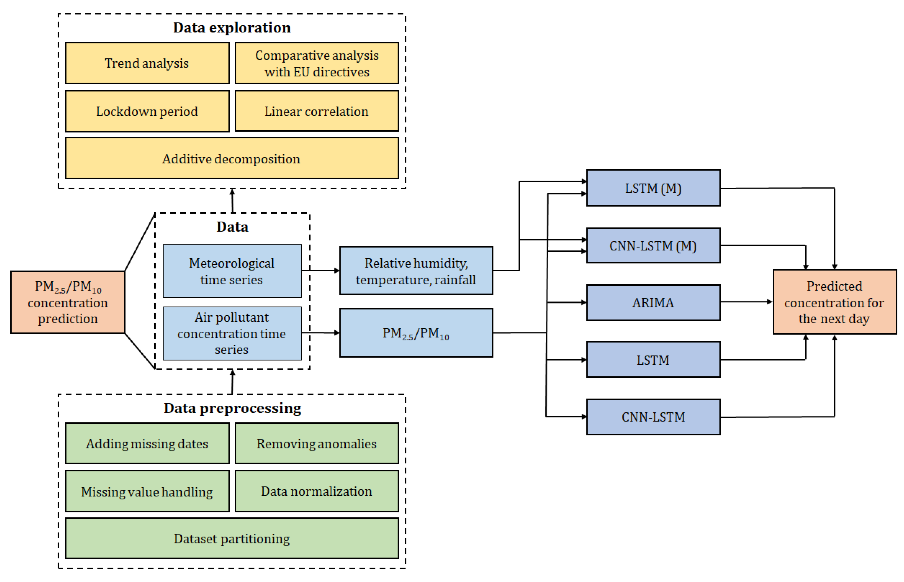
3. The Air-Pollution-Prediction Framework
Statistical models are employed in air quality forecasting due to their simplicity; they can predict future concentrations of air pollutants by assessing the relationship between these pollutants and past climatic parameters, without the knowledge of the pollution sources and underlying physical or chemical processes. Examples of classical statistical models for air pollution prediction include the Autoregressive Integrated Moving Average (ARIMA) model, multiple linear regression (MLR) model, and the Grey Model (GM).
This study rests on the air-pollution-prediction framework depicted in
Figure 1. The details are introduced in the remaining part of this section.
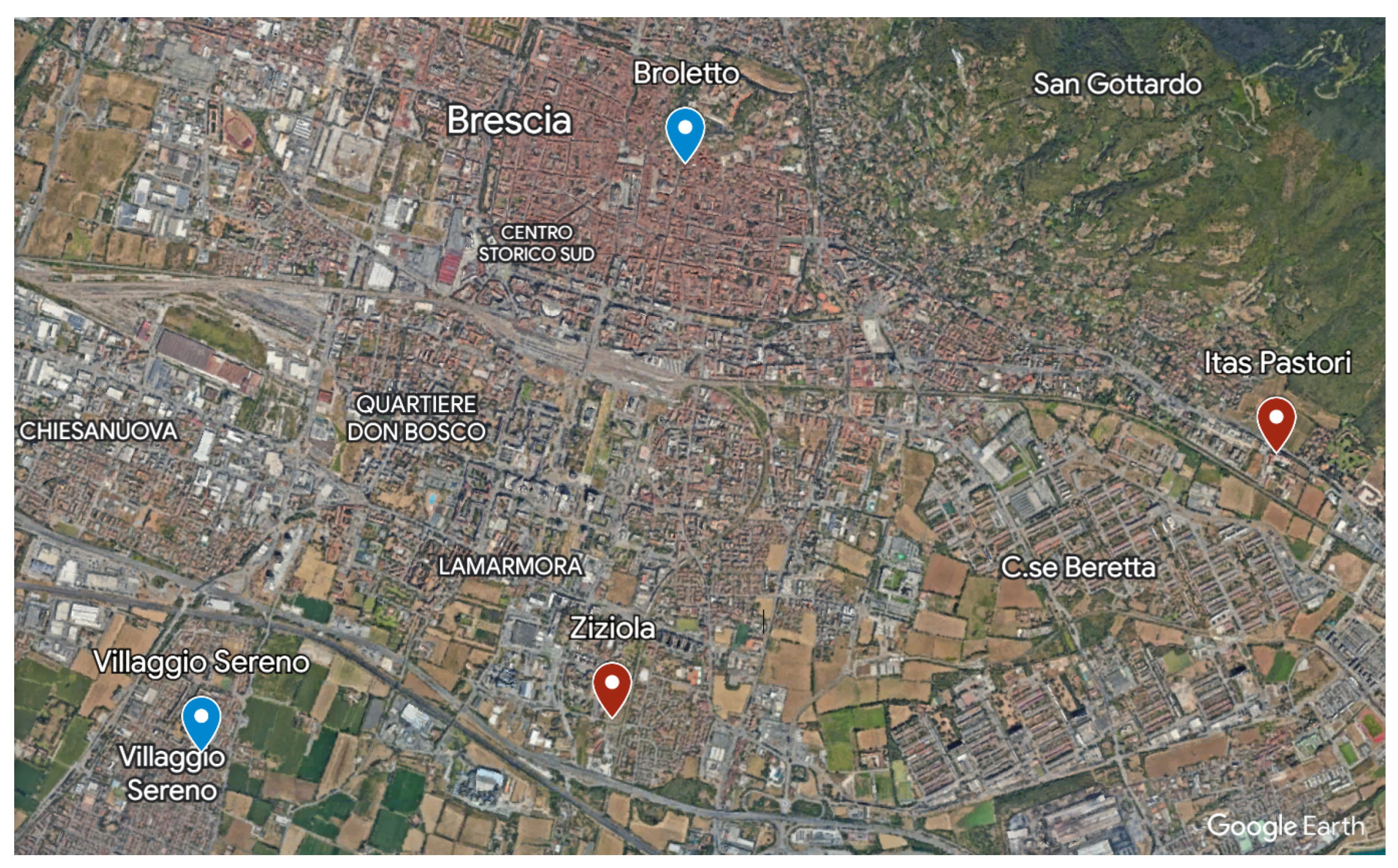
In detail, daily measurements of PM
10 (
g/m
) were utilized (
https://www.dati.lombardia.it accessed on 17 December 2023), originating from the monitoring station at via Broletto in Brescia. This station is situated in a location predominantly influenced by traffic emissions. Daily concentrations of PM
2.5 (
g/m
), as well as those of NO
, O
, PM
10, and SO
, from the Villaggio Sereno station, were also employed for a preliminary analysis of the major pollutants. The latter station is located in an area where pollution levels are not primarily determined by specific sources but by the integrated contribution of all sources upwind of the station concerning the prevailing wind directions at the site.
Meteorological data, including daily temperature (Celsius degrees), relative humidity (%), and rainfall (mm), were recorded at the Brescia Itas Pastori and via Ziziola weather stations. All time series cover the years from 2006 to 2022, except for PM2.5, which begins in 2007.
The locations of each station are indicated in
Figure 2.
3.1. Pre-Processing of Data
Data pre-processing is essential to prepare the data in a suitable input format for predictive models. The transformations applied are described below.
Firstly, some dates within the original time series were missing within the considered time frame. These missing dates were added, and no values were assigned to them. Subsequently, the presence of anomalous values was checked, and when found, these anomalies were removed. Anomalies refer to data points falling outside the acceptable value range for the variable under consideration, such as negative PM2.5 concentrations.
In the raw datasets, missing values were identified and had to be replaced, as the methods to be used require complete data. Additionally, there are consecutive observations without values that make the use of linear interpolation unrealistic for handling gaps in the time series. Regarding pollutant concentrations, replacements were made using the first available value from previous years on the same day and month as the missing measurement. In cases where there was no such value, subsequent years were examined.
For meteorological data, the station with the fewest missing values, namely Itas Pastori, was considered. These missing values were replaced by data obtained on the same date from the Via Ziziola station. The same technique used for pollutant concentrations was applied to the remaining missing values.
Finally, the data input for the neural-network-based models was normalized to improve predictions. The min–max normalization was used and is described by the following equation:
3.2. Predictive Models
While simple polynomial fitting may seem like an intuitive approach, it is often not feasible for several reasons. Air pollution is influenced by a multitude of factors, and their relationships are often non-linear. Simple polynomial fitting assumes a linear relationship between the input features and the output, which may not accurately capture the complex and non-linear nature of air pollution dynamics. Another aspect to be taken into account is that air quality datasets typically involve a high number of variables, such as meteorological conditions, traffic patterns, industrial activities, and more. Simple polynomial fitting might struggle to model the interactions among these variables effectively, especially when they exhibit non-linear dependencies.
It has to be noticed that simple polynomial models are prone to overfitting, especially when dealing with high-dimensional data. Overfitting occurs when a model fits the training data too closely, capturing noise rather than the underlying patterns. This can lead to poor generalization performance on new, unseen data. Furthermore, simple polynomials have limited expressiveness compared to more-advanced Machine Learning models. They may not be able to capture complex patterns, interactions, and dependencies present in the data, limiting their ability to make accurate predictions. Another problem with polynomial fitting assumes homoscedasticity, meaning that the variance of the errors is constant across all levels of the independent variable. In air pollution prediction, the variance of pollutants may not be constant, leading to violations of this assumption.
Finally, polynomial models can be sensitive to outliers, and air quality datasets may contain anomalous data points due to sensor errors, extreme weather events, or other factors. Simple polynomial fitting might be heavily influenced by these outliers, leading to biased predictions.
Table 8 summarises the cited models.
In this work, several models were implemented and compared for predicting concentrations of PM2.5 and PM10 for the next day. Three different methods were selected, belonging to different categories: ARIMA (statistical), LSTM network (Machine Learning), and CNN-LSTM (hybrid). For the neural networks, a multivariate variant was designed that included both meteorological and air quality data. The parameters for each model are specified below to achieve the best predictions.
The datasets were split into a training set (approximately 80% from 2006/2007 to 2019) and a testing set (approximately 20% from 2020 to 2022).
The ARIMA (4,1,2) and ARIMA (5,1,1) models were fit to the training data for the PM10 and PM2.5 concentrations, respectively. The parameters p, d, and q were determined using the ‘auto.arima’ function from the R ‘forecast’ library, which searches for the best ARIMA model within specified order constraints based on the AICc value.
With regard to the LSTM model, input data were created, consisting of sequences of seven consecutive days containing the pollutant concentration data to be predicted. In the multivariate model, meteorological data were added as additional features. The neural network structure included an LSTM layer with ReLU activation, composed of 16 neurons in the univariate model and 64 in the multivariate model. It was followed by a final dense layer with a single unit that holds the predicted value for the next day. The training of the network used the ‘adam’ optimizer, the mean-squared error as the loss function, a batch size of 128, and 50 epochs in the univariate case and 100 in the multivariate case.
In the hybrid CNN-LSTM model, all parameters were the same as in the LSTM, with the only difference being in the network architecture. The LSTM layer was preceded by a one-dimensional convolutional layer with 8 filters in the univariate case and 32 in the multivariate case, a kernel size of two, and ReLU activation. CNNs were initially developed for image processing, but have also been adapted for time series analysis. They can extract patterns and relevant features from time series data, including trends, cycles, peaks, and other significant information.
To evaluate the performance of predictive models, two indicators were used: mean absolute error (MAE) and root-mean-squared error (RMSE). These metrics are defined by the following equations:
where
is the predicted value,
is the actual value, and
n is the total number of observations.
The Pearson correlation coefficient was used to measure the linear relationship between two variables. It is defined as:
where
x and
y represent two variables,
and
are their means, and
n is the total number of observations. This coefficient was used to investigate the correlations between PM
2.5 and PM
10 concentrations and meteorological variables.
4. Experiments and Discussion
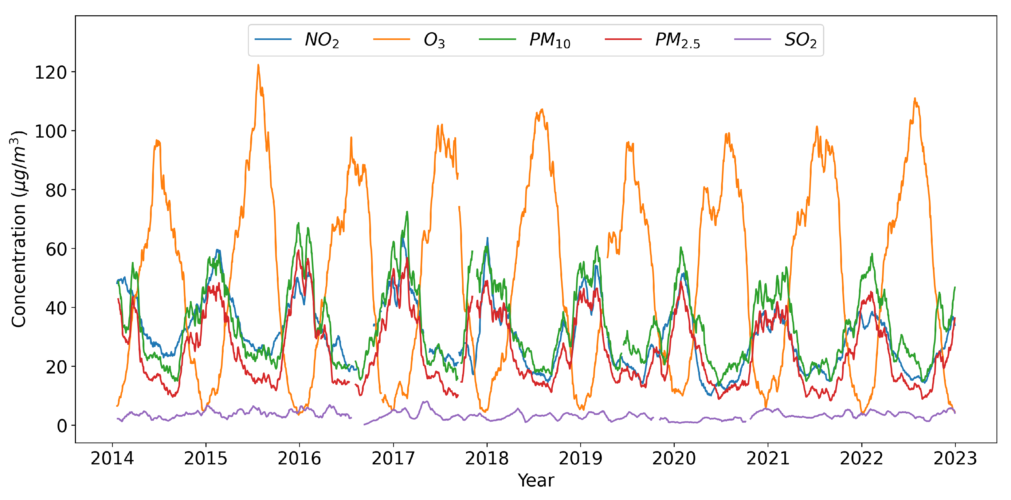
Initially, the trends in the major atmospheric pollutants in the city of Brescia from 2014 to 2022 were analyzed. A graph showing the trend is presented in
Figure 3, with a 30-day moving average applied to the data for visualization. The PM
2.5, PM
10, and NO
2 concentrations exhibited similar seasonal patterns, with peaks in colder months and moderate levels in summer. This is due to increased heating source usage in winter and the occurrence of temperature inversions, inhibiting vertical air mixing and favoring the accumulation of ground-level pollutants. Conversely, ozone showed an opposite seasonal pattern, forming due to chemical reactions between nitrogen oxides and volatile organic compounds, favored by high temperatures and intense sunlight. Sulfur dioxide appeared to lack a clear seasonal pattern.
Pollutant concentrations from 2014 to 2022 were compared to the limits set by the EU directives. In
Table 3, the annual average concentrations of PM
2.5, PM
10, and NO
2 are shown, with limit values of 25
g/m
and 40
g/m
.
The only pollutant that did not meet the threshold was PM
2.5 in the years from 2014 to 2018; however, it showed a decrease over time, as did NO
2. The last three columns of the table report the total number of days on which the limit values for PM
10 (50
g/m
, daily average), SO
2 (125
g/m
, daily average), and ozone (120
g/m
, maximum 8 h daily average) were exceeded. These values should not be exceeded for more than 35, 3, and 25 (averaged over 3 years) days per year, respectively. The SO
2 threshold has never been exceeded; on the other hand, PM
10 and ozone have not met the limits and did not show significant improvements over the entire period considered (see
Table 9).
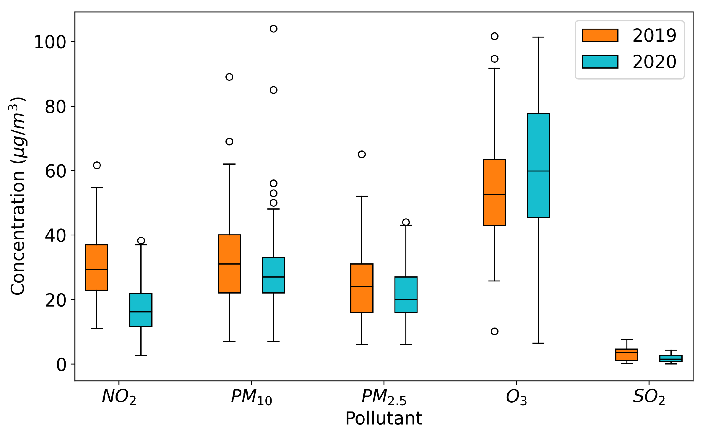
The health emergency caused by COVID-19 in Italy imposed a series of restrictions that affected both economic activities and the freedom of movement of citizens, with uneven effects on air quality in Brescia. In
Figure 4, boxplot graphs illustrate the concentrations of each pollutant in the months of March and April in 2020 (the lockdown period) and 2019.
Despite significant reductions in emissions, especially related to the transportation sector and, to a lesser extent, energy production, industrial activities, and livestock, the decreases in pollutant concentrations varied depending on the pollutant considered: much more pronounced for NO, less noticeable for PM10, PM2.5, and SO, and absent for O. The effects on nitrogen dioxide were more pronounced because it is directly linked to traffic emissions. In contrast, the lesser impact on ozone and sulfur dioxide levels was due to the fact that the former is a secondary pollutant without significant direct emission sources and the latter typically has very low concentrations. The case of atmospheric particulate matter demonstrated the complexity of the phenomena involved, related to formation, transportation, and accumulation.
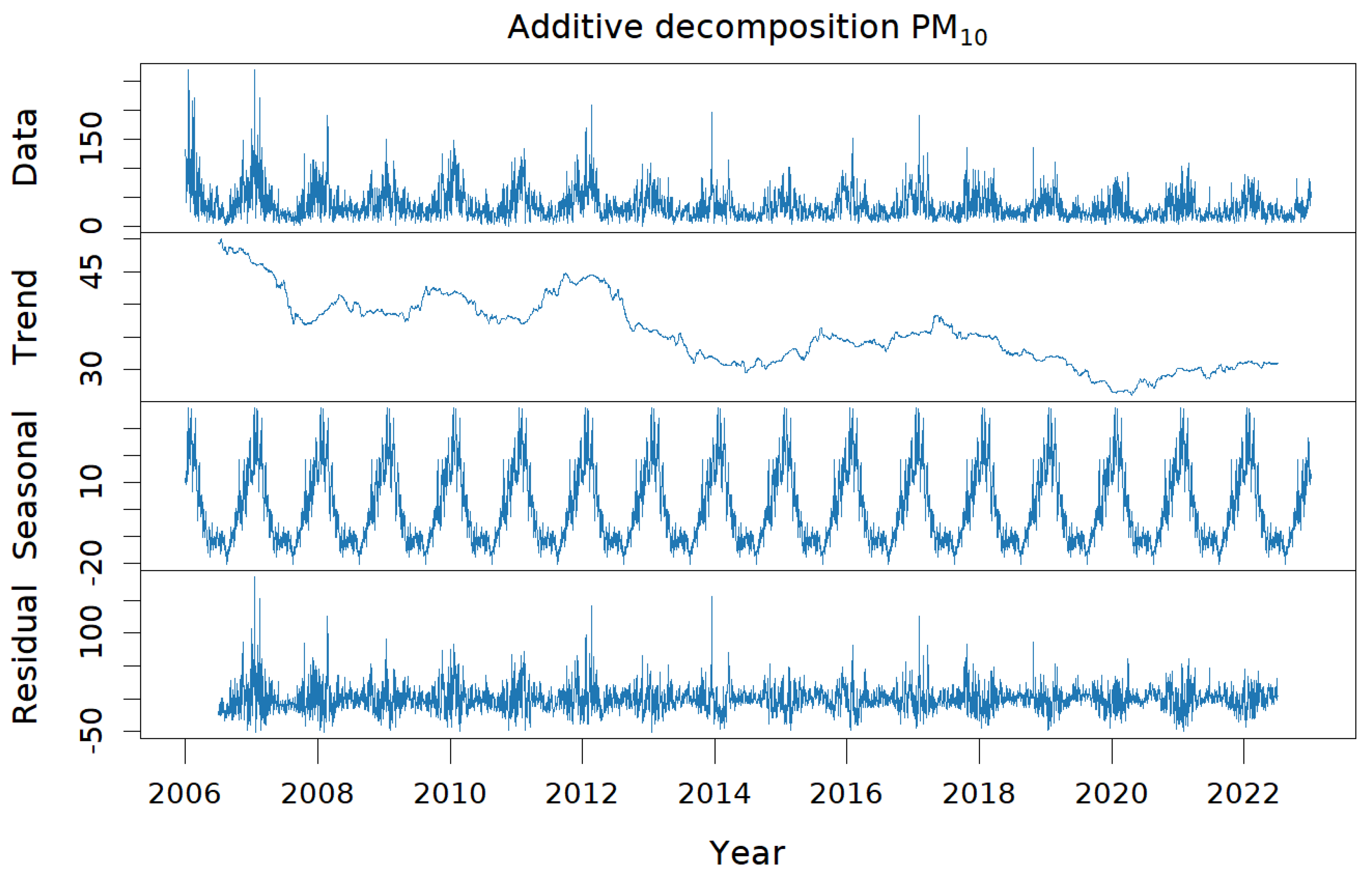
Focusing solely on PM
2.5 and PM
10, an additive decomposition was applied to their respective time series. In
Figure 5, the graph shows the concentration of PM
10 and its corresponding trend, seasonal, and residual components, which were very similar to those obtained for fine particulate matter. Both pollutants exhibited clear seasonality, as deduced previously, and a decreasing trend. Therefore, the time series were not stationary. In particular, the PM
10 trend was less regular and showed a slight increase in the recent period compared to that of PM
2.5. The residual part was significant in both cases.
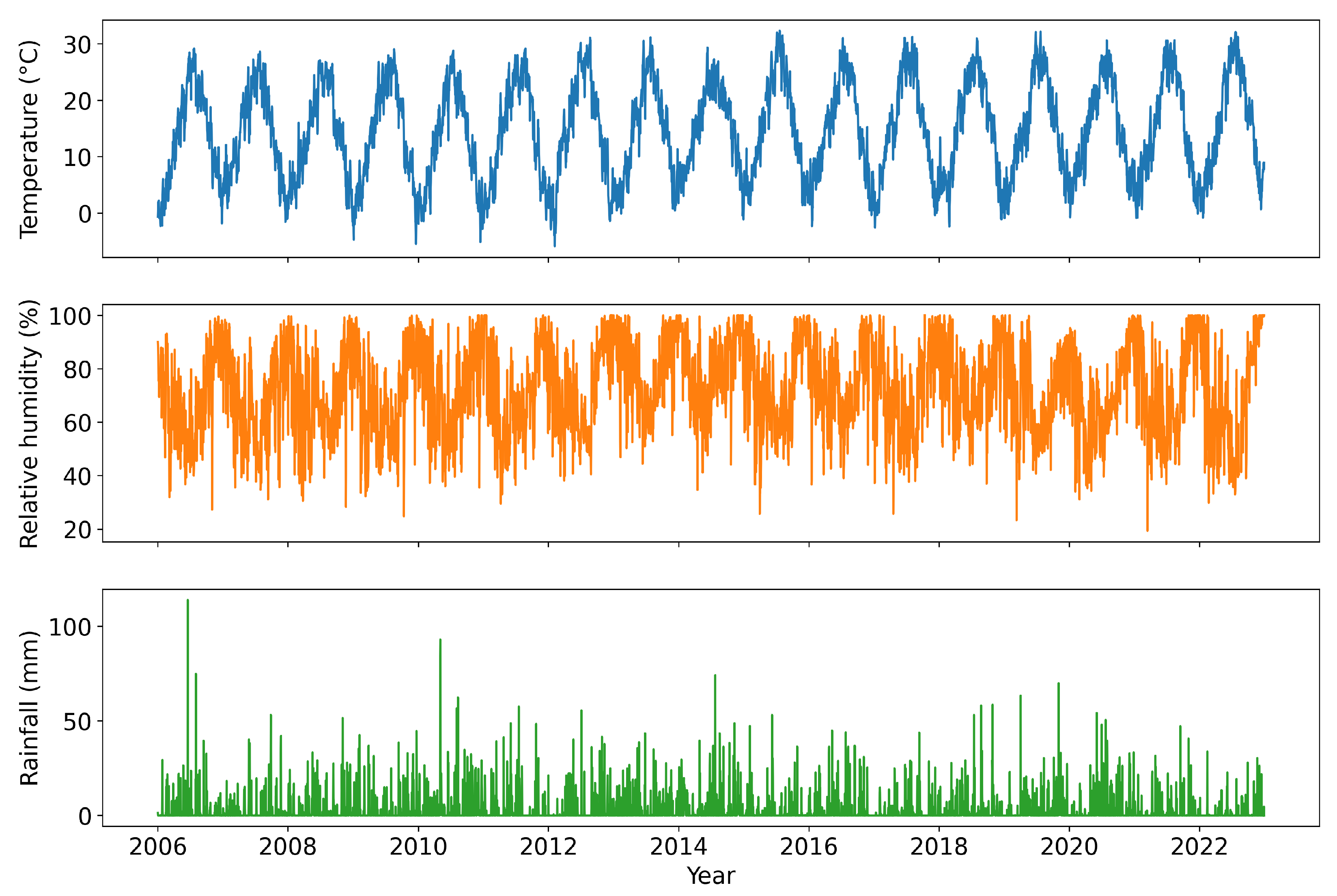
We then proceeded to analyze the linear correlation between the two pollutants and meteorological variables, reporting the measurements in
Table 10. Temperature showed the strongest correlation, followed by relative humidity and rainfall. The seasonality of relative humidity was the same as that of atmospheric particulate matter, explaining the positive correlation. The opposite was true for temperature. Temporal weather data from 2006 to 2022 are illustrated in
Figure 6.
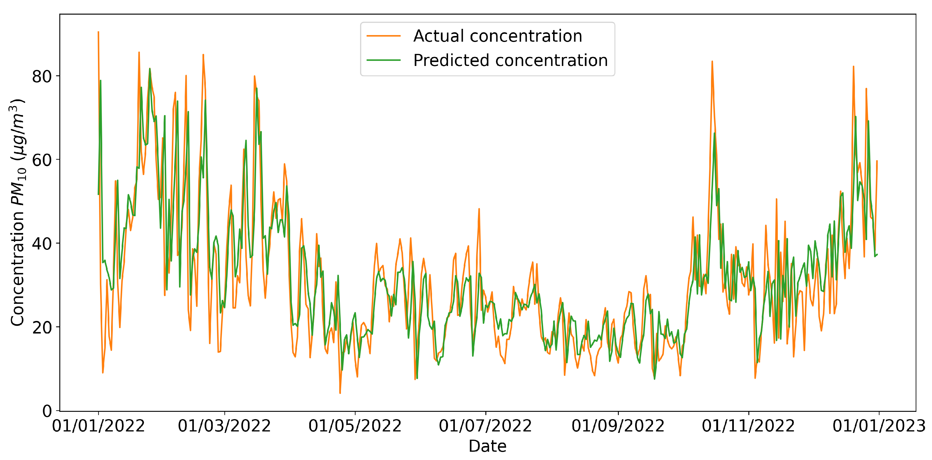
In the final step of this study, the concentration of the next day’s atmospheric particulate matter was predicted using the aforementioned models adapted to the training data. Their performance was measured using the evaluation metrics RMSE and MAE, where the former will assume a higher value compared to the latter as it assigns more weight to large errors.
From
Table 11, it can be observed that all models achieved reasonable results; the multivariate CNN-LSTM network performed the best. In
Figure 7, the predictions of PM
10 made by the neural network for the 2022 testing data and the actual daily concentration values are represented.
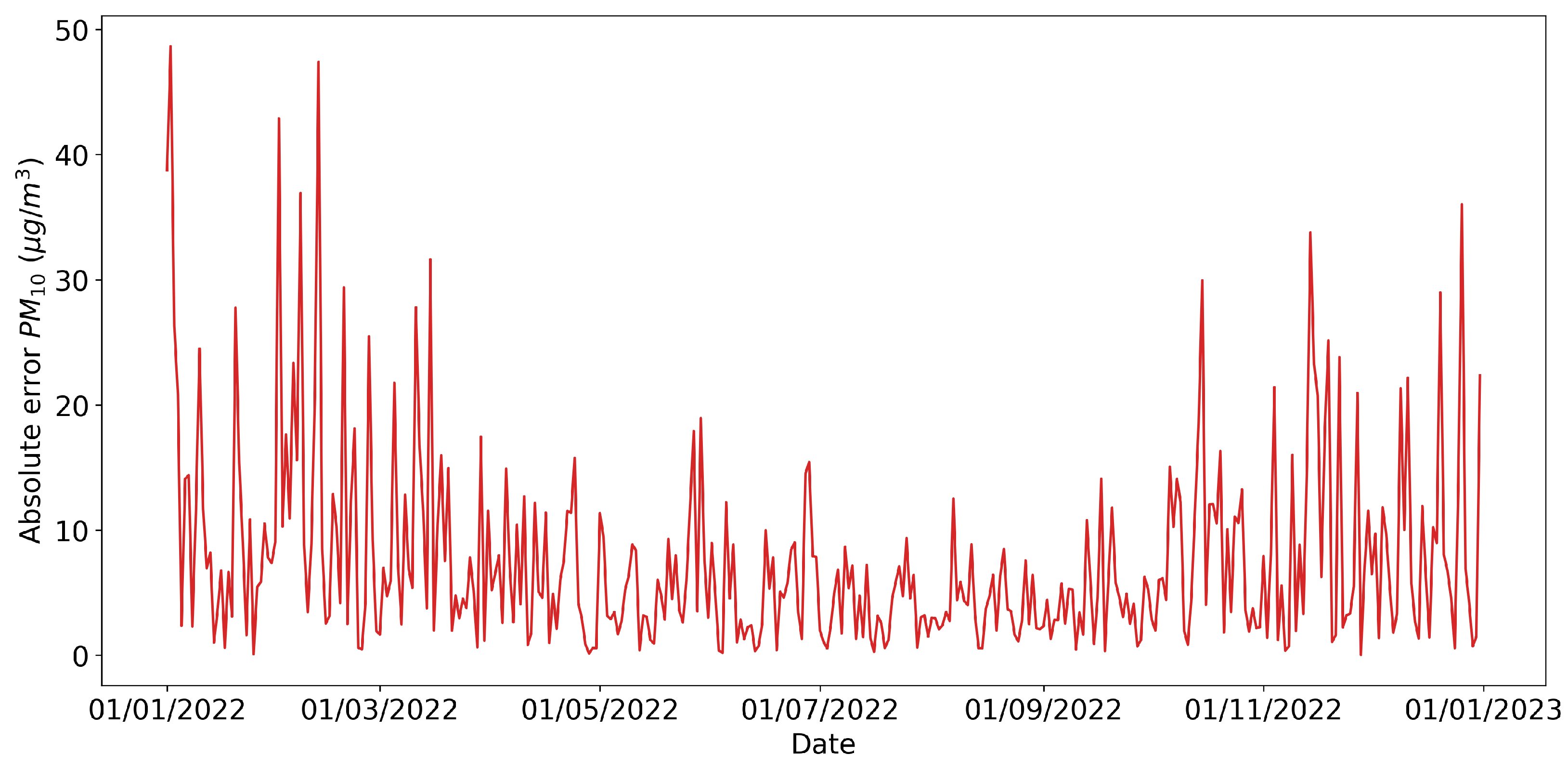
The absolute error of each prediction is shown in
Figure 8 and reached its highest values in the months when the concentration of PM
10 showed significant peaks.
For further comparison among the various methods, the execution times required for the training phase related to the PM
10 data are reported in
Table 12.
In general, the multivariate models outperformed the univariate models: considering additional relevant features, such as weather data, helped provide more-accurate predictions.
The CNN-LSTM model, compared to the LSTM network, did not lead to significant improvements in either the training or testing data: the convolutional layer was unable to extract additional useful information for prediction, a task made challenging by the high variability of the data and the low number of observations available.
Furthermore, it can be observed that the scores related to PM2.5 were lower compared to those of PM10 because the data for the latter had a higher standard deviation (25.06 g/m for PM10 and 20.18 g/m for PM2.5), making the prediction more challenging. A difference was also observed between the training and testing data as they referred to time intervals of different lengths.
Additional tests were conducted by extending the input data window of the neural networks to 14 and 30 days. The results showed that the prediction error remained almost unchanged, and the training time increased compared to the original case of 7 days. The same outcome was obtained when exploring the addition of two more features in the multivariate models: the month and day of pollutant concentration measurement. The inclusion of this temporal information did not improve the accuracy of trend prediction, proving to be irrelevant features.
5. Conclusions
In this article, the problem of modeling and forecasting the amount of air pollution in the smart city of Brescia was presented, highlighting several important aspects related to it, such as natural and anthropogenic sources, the dispersion mechanisms, and the environmental and human health implications. Time series data have proven to be a fundamental tool for describing pollutant concentrations over time. They can reveal trends, seasonal and cyclic behaviors, and the crucial property of stationarity. Subsequently, ARIMA and LSTM models suitable for forecasting future values of a time series were introduced. Both models attempt to represent autocorrelation in the data, the former through linear relationships with past values of the series and white noise, including the differencing operation, and the latter through hidden states and recurrent connections. Part of the work was dedicated to the state-of-the-art to provide an overview of current studies related to air pollution forecasting, which were categorized based on the type of model implemented (statistical, Machine Learning, physical, and hybrid).
Finally, pollutant concentrations in Brescia were analyzed using the aforementioned tools. Thanks to the results obtained, it is now possible to answer the question posed in the Introduction of this work.
Regarding the current state of air quality, in 2022, the pollutants with the most-critical levels recorded at the Villaggio Sereno (BS) station were PM
10 and ozone, with 60 and 92 days of exceeding the EU limits, well above the maximum allowable 35 and 25 days of excess. Although PM
2.5 complied with the EU thresholds, it reached levels in 2021 and 2022 that ranked among the worst in all of Europe, as stated in the latest report from the EEA [
7]. The data related to NO
and SO
were not concerning.
The decreasing trend of particulate matter from 2006 to 2022, as well as the decrease in the average annual concentration of nitrogen dioxide between 2014 and 2022 indicated that there has been an improvement compared to previous years. However, the same cannot be said when considering the total days of exceeding ozone and PM10 in a year.
As for predicting concentrations, this is a task that can be far from simple if accurate results are desired. The predictions of PM2.5 and PM10 for the next day, calculated using the ARIMA, LSTM, and CNN-LSTM models on the testing data, were not perfect. However, they were considered reasonable since the concentration values can vary significantly from one day to the next, making the situation considerably more complex. PM2.5 had lower RMSE and MAE scores compared to PM10, precisely because it had a smaller standard deviation.
The high variability of particulate matter demonstrated how intricate the phenomena involved are. Further evidence of this complexity was provided by the analysis of the lockdown period due to COVID-19, where, despite significant reductions in emissions, equivalent decreases in the PM
2.5 and PM
10 concentrations were not observed. It is worth mentioning a study conducted by Shi et al. [
32]: alterations in emissions correlated with the initial 2020 COVID-19 lockdown restrictions resulted in intricate and substantial shifts in air pollutant levels; however, these changes proved to be less extensive than anticipated. The reduction in nitrogen dioxide (NO
) is anticipated to yield positive effects on public health, yet the concurrent elevation in ozone (O
) levels is expected to counteract, at least partially, this favorable outcome. Notably, the scale and even the direction of variations in particulate matter with a diameter of 2.5
m or less (PM
) during the lockdowns exhibited marked disparities across the scrutinized urban locales. The involvement of chemical processes within the mixed atmospheric system introduces complexity to endeavors aimed at mitigating secondary pollution, such as O
and PM
, through the curtailment of precursor emissions, including nitrogen oxides and volatile organic compounds (VOCs). Prospective regulatory measures necessitate a systematic approach tailored for specific cities concerning NO
, O
, and PM
, accounting for both primary emissions and secondary processes. This approach aims to optimize overall benefits to air quality and human health.
One solution for achieving better predictions may be the inclusion of additional variables that help explain the pollutant’s behavior further, as was the case in the implemented multivariate models.
In the future, aspects that were not addressed in this research could be further explored. Firstly, to improve the results, additional variables related to weather, traffic, and other pollutants could be considered or different models could be used. New methods for providing long-term forecasts, limited here to the following day, could be investigated, and data with a different granularity than daily could be employed.
Secondly, factors such as natural and anthropogenic sources, dispersion mechanisms, and environmental and human health implications will be addressed in the light of the performed experiments.


