MultiWave-Net: An Optimized Spatiotemporal Network for Abnormal Action Recognition Using Wavelet-Based Channel Augmentation

Abstract

Human behavior is regarded as one of the most complex notions present nowadays, due to the large magnitude of possibilities. These behaviors and actions can be distinguished as normal and abnormal. However, abnormal behavior is a vast spectrum, so in this work, abnormal behavior is regarded as human aggression or in another context when car accidents occur on the road. As this behavior can negatively affect the surrounding traffic participants, such as vehicles and other pedestrians, it is crucial to monitor such behavior. Given the current prevalent spread of cameras everywhere with different types, they can be used to classify and monitor such behavior. Accordingly, this work proposes a new optimized model based on a novel integrated wavelet-based channel augmentation unit for classifying human behavior in various scenes, having a total number of trainable parameters of 5.3 m with an average inference time of 0.09 s. The model has been trained and evaluated on four public datasets: Real Live Violence Situations (RLVS), Highway Incident Detection (HWID), Movie Fights, and Hockey Fights. The proposed technique achieved accuracies in the range of $92\%$ to $99.5\%$ across the used benchmark datasets. Comprehensive analysis and comparisons between different versions of the model and the state-of-the-art have been performed to confirm the model’s performance in terms of accuracy and efficiency. The proposed model has higher accuracy with an average of $4.97\%$, and higher efficiency by reducing the number of parameters by around 139.1 m compared to other models trained and tested on the same benchmark datasets.

1. Introduction

There has been an increased usage of cameras worldwide, which helps significantly in monitoring a larger number of events, particularly where a conflict or hostile actions can be detected. Some of the events that a camera captures can be considered irregular, which can be defined as something anomalous or divergent from normal events. For example, humans fighting or engaging in hostile acts. Surveillance cameras record these events without any discrimination, which leaves security and law enforcement personnel to decide after a lengthy period the final verdict, however, this results in a delay in response times to such events. There have been several investigations conducted by the authors related to integrating artificial intelligence techniques into the obtained camera data for various purposes as in [1]. Since both traditional image processing and deep learning techniques have their limitations, there is a need for the combination of both to increase robustness.

Here, in this paper, an issue that is related to the safety measures that a camera can provide is discussed. A deep learning model is proposed that integrates a novel concept of channel augmentation in the wavelet domain while using an efficient neural network structure that empowers the model in terms of performance in real-time and accuracy at the same time.

Since both traditional image processing and deep learning techniques have their limitations, there is a need for the combination of both to increase robustness. Wavelet transform is one of the important applications in digital image processing. There have been several approaches performed by the authors that used different types of wavelet transforms with different filter designs for multiple applications as in [2,3]. Lately, a lot of methodologies that combined wavelets with Deep learning as in [4,5,6,7,8] were proposed which made such approaches to be used in many applications as in [9,10,11,12].

In [13], the authors emphasize on how the high frequency component can be an important factor for the generalization capability of a CNN. Moreover, most of the work performed in the anomaly recognition application uses models that extract features from RGB images. The previous work of the other authors that combines wavelets and deep learning paved the way for the proposed approach to integrating the wavelet transform in the model proposed for abnormal action recognition.

The proposed model comprises of four parts. The first one is the novel unit called Integrated Serial Channel Augmentation (ISCA), using different wavelet transform techniques, namely Discrete Wavelet Transform (DWT), Discrete Multi-Wavelet Transform (DMWT), and Dual-Tree Complex Wavelet Transform (DTCWT). DWT is the basic known wavelet decomposition for images, the other two types are used to see if these techniques provide better accuracies when they counter the limitations of DWT. These generated channels are further combined with a thresholding technique to filter out the noise information in the high frequency component. The second part is applying general domain transfer learning on MobileNetV2 and using it as a spatial feature extractor. The third part is temporal feature extraction using Convolutional LSTM. The fourth part is using fully connected neurons for classification. Various versions of the ISCA block were made and compared against each other to prove that using a combination of multiple wavelet transform techniques to obtain different features is better than using the same wavelet transform techniques for obtaining features. The best-performing version of the proposed model is compared to other models in the state-of-the-art.

In short, the main aspects of this work include:

• A novel integrated serial channel augmentation (ISCA) block to generate wavelet-transformed images for feature extraction to mitigate the trade-off between accuracy and efficiency.
• The combination of the optimized MobileNetV2 CNN architecture with ConvLSTM for spatiotemporal classification.
• A detailed experimental study to prove the importance of each part of the network used with the proposed ISCA block in the form of an ablation study.
• Competitive performance compared to the current state-of-the-art models across different benchmark datasets in terms of accuracy and efficiency defined as the number of trainable parameters.

The remaining sections of this paper are organized as follows: In Section 2, some work related to action recognition is presented, with some focus on the abnormal and violent action recognition application. There is also a brief discussion about the current state-of-the-art along with the direction of this paper. In Section 3, the proposed model is introduced in detail. In Section 4, the results obtained and experiments performed using holdout and cross-validation with different versions of the model are shown. An ablation study is also conducted to prove the effectiveness of each part in the network. There is also a comparison with other methods on the different datasets used. In Section 5, the conclusion and future work are presented.

2. Related Work

In this section, the main approaches were explored in the current state-of-the-art, that are being used for human activity and abnormal events recognition.

2.1. Image Processing and Machine Learning Approaches

In [14], the authors proposed a novel average energy image (AEI) feature descriptor by using HOG and PCA with AEI. In [15], they introduced a framework that can make a feature vector by using R-transform and Zernike moments on average energy silhouette images (AESIs). In [16], they proposed a framework that applies a feature vector unifying both global and local information to strengthen the extraction of unique features for action recognition. While in [17], an algorithm was proposed that starts by testing two different object detectors, a Haar cascade detector, and a faster region convolutional neural network for human detection. Both models were trained using publicly available datasets. The actions were classified using the supervised machine learning algorithm called Support Vector Machine. Finally, actions with low scores were considered anomalous.

2.2. CNN Spatial-Based Approaches

In [18], they proposed a CNN-based method for abnormal behavior detection. The method automatically learned the characteristics concerning a wide range of abnormal behaviors. While others tried to extend the CNN dimensionality as in [19,20], they proposed a new novel Convolutional Neural Network (3D-CNN) with 3D motion cuboid for action detection and recognition in videos. In [21,22,23], they tried to make a combination of residual connections and 2D-CNNs. Lastly, in [24], the authors proposed an architecture of residual blocks based on ResNet50 that were used with 3D-CNNs to obtain spatiotemporal representative features from videos.

2.3. CNN and Sequence Models Approaches

In [25], the authors proposed an architecture consisting of two convolutional layers and one convolutional LSTM layer with fully connected layers for classification. In [26], a model was proposed that consisted of a spatial feature extractor that follows the U-Net network structure by using MobileNetV2 as an encoder for spatial feature extraction, followed by LSTM for temporal feature extraction. In [27], a new model was proposed that had a multi-head self-attention layer, and a bidirectional long short-term memory to encode relevant spatiotemporal features, to classify whether a sequence of frames showed violence or not. In [28], the authors tried to combine 3D convolution with late temporal modeling so they used the TGAP layer after the 3D convolutional layers with the bidirectional encoder representations from transformers’ (BERT) attention mechanism. In [29], they proposed a model that extracted spatiotemporal features by using a CNN and LSTM. The classification was performed using a fully connected neural network to classify the video into violent or non-violent actions. In [30], they proposed a framework of two parts. First, spatial features were extracted from the frames of the video using CNN with a leap in the sequence of frames Second, the features extracted from the sequence were handed to DB-LSTM in flattened small pieces. Lastly, in [31] they discovered that the classic LSTM could strengthen the deterministic features of human actions to reflect the change in speed. Thus, an improved LSTM structure was proposed.

2.4. Wavelet-Based Approaches

In [32], they proposed a 3D stationary wavelet transform to encode the spatiotemporal characteristics of the motion happening in a sequence of frames similar to motion history images. In [33], they extended their work by combining SWT with a local binary pattern histogram and Hu invariant moments for the global representation of motion. In [34], the authors proposed an architecture that combined discrete wavelet transform along with CNN and Bidirectional LSTM (BiLSTM) to classify image sequences. In [35], they proposed a method that combined the usage of continuous wavelet transform and CNNs.

2.5. Transformers Approaches

In [36], the authors introduced a method that used a transformer model that worked with 2D images. It worked by applying CNN first to learn spatial features, then adding temporal information in the data stream using an attention model approach to the spatial features. While in [37], they used an action transformer that can extract and combine all human-specific features in the video. The proposed architecture was composed of two networks: the base, and the head. A 3D-CNN architecture was applied to obtain features that were sent to the Region Proposal Network to obtain potential object candidates.

2.6. Discussion on Literature and Research Gap

From the comprehensive literature review performed, it is noticed that most of the work uses very deep architectures that are inefficient. In

Table 1. Main highlights of the current approaches in the literature.

Methods	Reference(s)	Strengths	Weaknesses
Image Processing and Machine Learning	[38]	Computationally light, depending on the algorithm complexity used.	Poor generalization capability depending on the application and scenarios tackled.
CNN and Sequence Models	[39]	They can have good classification accuracy and can be computationally light depending on the number of layers used. They also can adapt to new data.	They can be memory demanding for training if the sequence length used for training is large. They can easily overfit/underfit data during training depending on the training setting used.
Spatiotemporal 3D CNN	[40]	Good classification accuracy, and can adapt to new data.	Some architectures are computationally extensive, while others lack effective representation.
Transformers	[41]	Good classification accuracy, and can adapt to new data.	Computationally extensive, due to the large number of trainable parameters, and the self-attention mechanism that processes long sequences of data at once.

, an overview of some of the current state-of-the-art methodologies used is mentioned. The table shows the main strengths and drawbacks while providing a reference for full reviews of such approaches.

After observing the state-of-the-art, it is decided to utilize the CNN and sequence modeling approach, while trying to mitigate the challenges related to them by integrating a novel combination of ISCA wavelet-based block with MobileNetV2 and a special type of LSTM called Convolutional LSTM. The idea from the ISCA block is to perform wavelet transform and concatenating all the subbands that come out of a transform together using a single layer unlike other approaches in the literature that only use certain coefficients.

The main advantage of our approach is that integrating the wavelet-based ISCA block with a light CNN enhances the model’s efficiency, as all the wavelet transform techniques run with a time complexity of $O\left(N\right)$ as they are implemented in a separable manner. These wavelet blocks also enhance the optimization process by using a computationally efficient network that uses depthwise separable convolutions called MobileNetV2 and underperforms with models with more parameters. The ConvLSTM is used to capture local spatiotemporal features in each frame in the sequence making them the most suitable choice for this application.

3. Materials and Methods

This section introduces the main components used in the proposed model, then showcases and discusses the whole pipeline as shown in Figure 1. The first block shows how the videos in the dataset are sampled to obtain a more efficient representation of them. The second block describes the wavelet-based channel augmentation using different wavelet transform techniques. The third block shows the spatial feature extraction process using MobileNetV2. The fourth block shows the temporal feature extraction process using Convolutional LSTM. Finally, the last block is the one that classifies the features extracted from the previous blocks using fully connected neurons.

3.1. Video Segmentation Using Sparse Sampling

In this section, the data is prepared to be in a spatiotemporal format for training the model. This is performed by reading frames from a video with a skip window. Since the videos in the datasets are short and focus on the actions that should be detected later on, it is important to give these videos an efficient representation by selecting frames throughout the video duration. In order to capture the whole action in different time instances, each frame is converted to be monochromatic, resized to a certain size, and then normalized. This process is performed iteratively for each video in the dataset, where each video is represented in a sequence of 16 frames. In order to select the 16 frames, sparse sampling is applied to each video in a dataset. Sparse sampling defines a fixed interval $Maximum(\tau =\frac{\nu }{16},1)$ that is used to select the frames from a video, where $\tau$ is the sampling window, and $\nu$ is the total number of frames in a video.

3.2. Wavelet Transform

Wavelet Transform (WT) [42] is an arithmetical model proposed to resolve the issue of non-stationary signal decomposition. Based on the authors’ hypothesis in [13], different WT techniques are used. The reason for that is to expose the high frequency components of the frames for the CNN spatial feature extractor in the next phase to learn features based on them. Three different wavelet transform techniques were used in this approach to generate three channel inputs for the CNN spatial feature extractor namely Discrete Wavelet Transform (DWT), Dual-Tree Complex Wavelet transform (DTCWT), and Discrete Multi-Wavelet Transform (DMWT). The different transform techniques output different coefficients with different properties as shown in Figure 2.

3.2.1. Discrete Wavelet Transform

To adjust to discrete 2D data like images, DWT [43] was introduced to decompose images into components with different frequency intervals. In this work, a typical 2D-DWT is used on images using the Haar wavelet in a filter bank approach. The 2D-DWT is performed in a separable manner. The output of DWT is two coefficients. The approximation coefficient (low frequency) information is denoted as $LL$. Detail coefficients (high frequency) are the horizontal edges denoted as $LH$, vertical edges denoted as $HL$, and finally, diagonal edges denoted as $HH$. The frequency components are $1/4$ the size of the original images. The $LL$, $LH$, $HL$, and $HH$ components are concatenated so that the output image with the different subbands is the same size as the input image. If X is an input image, the concatenation method can be shown in the matrix below (1):

$$DWT\left(X\right)=\left[\begin{array}{cc}LL& LH\\ HL& HH\end{array}\right]$$

(1)

Unlike other types of transform, DWT has adaptable time-frequency resolution, but it also has some drawbacks. The DWT is insufficient in terms of direction selectivity as it only has three directions. Also, the downsampling operation in the DWT filter bank design causes high rates of distortion, thus it is shift-variant.

3.2.2. Dual-Tree Complex Wavelet Transform

The DTCWT [44] originally proposed by Kingsbury has good properties of approximate shift-invariance and good direction selectivity, which in turn helps in overcoming the limitations of DWT. Usually, a DTCWT filterbank structure can be looked at as two trees of DWT. The scaling and wavelet filters of one tree must generate functions that are approximate Hilbert transform of the scaling function and wavelet generated by its corresponding filters of the other tree. Therefore, the complex-valued scaling functions ${\Phi }_h\left(t\right)$${\Phi }_g\left(t\right)$ and wavelet functions ${\Psi }_h\left(t\right)$${\Psi }_g\left(t\right)$ formed from the two trees are approximately analytic and written as a Hilbert pair as shown in Equations (2) and (3).

$$\Psi \left(t\right)={\Psi }_h\left(t\right)+j{\Psi }_g\left(t\right)$$

(2)

$$\Phi \left(t\right)={\Phi }_h\left(t\right)+j{\Phi }_g\left(t\right)$$

(3)

where $\Psi (.)$ and $\Phi (.)$. When applied separably on 2D data, we obtain 2D complex separable wavelets and a 2D complex separable scaling function. They are implemented by separable filters along columns and then rows. Performing a 2D DTCWT decomposition, subband images can be obtained with more directions with phase shifts of ±15°, ±45°, ±75°. For an input image of size N × N, the output is a tensor of shape 2N × 2N.

3.2.3. Discrete Multi-Wavelet Transform

DWT is considered a single wavelet, as it has only one scaling and one wavelet function. This can limit the time-frequency resolution decomposition because a single wavelet function has a fixed support length. On the other hand, multi-wavelets contain more than one scaling function and wavelet function. The set of scaling functions can be written using vector notation as $\Phi \left(t\right)={[{\Phi }_1\left(t\right){\Phi }_2\left(t\right)\dots {\Phi }_r\left(t\right)]}^T$, where $\Phi \left(t\right)$ is called a multiscaling function. Similarly, the multiwavelet function is defined from the set of wavelet functions as $\Psi \left(t\right)={[{\Psi }_1\left(t\right){\Psi }_2\left(t\right)\dots {\Psi }_r\left(t\right)]}^T$, where $r>1$ is a positive integer, and it represents the number of scaling or wavelets functions used. When $r=2$, the multiwavelet two-scale equations can be defined as follows:

$$\Phi \left(t\right)={\Sigma }_{k=0}^{m-1}{G}_k\Phi (2t-k)$$

(4)

$$\Psi \left(t\right)={\Sigma }_{k=0}^{m-1}{H}_k\Phi (2t-k)$$

(5)

where the pair {$G_k,H_k$} is called a multiwavelet filter bank. $G_k$ is called a matrix low pass filter and $H_k$ is called a matrix high pass filter. They are $r\times r$ matrices for each integer k, and m is the number of scaling coefficients.

In this work, GHM multiwavelet [45] is used, where both the scaling and wavelet functions are orthogonal and symmetric. The GHM scaling and wavelet functions are as follows:

$$\Phi \left(t\right)=\sqrt{2}{\Sigma }_{k=2}^{}{G}_k\Phi (2t-k)$$

(6)

$$\Psi \left(t\right)=\sqrt{2}{\Sigma }_{k=2}^{}{H}_k\Phi (2t-k)$$

(7)

The filter banks pair {$G_k,H_k$} are defined with $k=2$. The matrices that contain different kernels for the GHM multiwavelet in this pair are $h_0$, $h_1$, $h_2$, $h_3$, $g_0$, $g_1$, $g_2$, $g_3$ each matrix is of size $2\times 2$. $h_0$, $h_1$ can be concatenated vertically to be of size $2\times 4$ and given a notation of ${\mathit{H}}_{\mathbf{1}}$, similarly for $h_2$, $h_3$, $g_0$, $g_1$, $g_2$, and $g_3$ give them a notation of ${\mathit{H}}_{\mathbf{2}}$, ${\mathit{G}}_{\mathbf{1}}$, ${\mathit{G}}_{\mathbf{2}}$, respectively. They are defined as follows:

$$H_1=\left[\begin{array}{cccc}3/5\sqrt{2}& 4/5& 3/5\sqrt{2}& 0\\ -1/20& -3/10\sqrt{2}& 9/20& 1/\sqrt{2}\end{array}\right]$$

(8)

$$G_1=\left[\begin{array}{cccc}-1/20& -3/10\sqrt{2}& 9/20& -1/\sqrt{2}\\ 1/10\sqrt{2}& 3/10& -9/10\sqrt{2}& 0\end{array}\right]$$

(9)

$$H_2=\left[\begin{array}{cccc}0& 0& 0& 0\\ 9/20& -3/10\sqrt{2}& -1/20& 0\end{array}\right]$$

(10)

$$G_2=\left[\begin{array}{cccc}9/20& -3/10\sqrt{2}& -1/20& 0\\ 9/10\sqrt{2}& -3/10& -1/10\sqrt{2}& 0\end{array}\right]$$

(11)

The kernels can be convolved with the input image in a filter bank approach to perform the wavelet decomposition just like the single wavelet decomposition to obtain different frequency components as shown in the matrix below (12).

$$DMWT\left(X\right)=\left[\begin{array}{cccc}{L}_1{L}_1& L_2{L}_1& L_1{H}_1& L_2{H}_1\\ L_1{L}_2& L_2{L}_2& L_1{H}_2& L_2{H}_2\\ H_1{L}_1& H_2{L}_1& H_1{H}_1& H_2{H}_1\\ H_1{L}_2& H_2{L}_2& H_1{H}_2& H_2{H}_2\end{array}\right]$$

(12)

The output tensor is of shape 2N × 2N, where N is the input size, and each subband has a certain frequency component. Each frequency component is divided to have shapes of N/4 × N/4, as all variations of the four filters are applied and then concatenated together.

3.3. Spatial Feature Extraction and Transfer Learning

Spatial features would be features that exploit location information. That can be performed using CNN by performing convolutions to extract spatial features in different locations of the image. Deep networks use filters to extract features; these features tend to be more complex layer by layer as we go into the depth of the neural network.

Transfer learning has many types and approaches, as shown in [46]. It can be useful when using a CNN backbone structure pre-trained on large datasets. The main benefit here is that, if the model is trained originally on a large and general dataset like ImageNet [47], one can take advantage of the trained weights up to a certain layer, and then add other classifying layers and jointly train them together. This process is called fine-tuning.

In this work, this idea is mainly used to preserve the CNN ability to extract low-order feature representations successfully, which are basically edges of different orientations. The CNN backbone used for the proposed model is MobileNet [48] pre-trained on the large-scale dataset ImageNet used for image classification. It has 53 layers to perform the fine-tuning; only the first 13 layers are frozen, and the rest are trained along with the other parts of the model. MobileNetV2 consists of three types of convolutional layers in the block as shown in Figure 3.

The first layer which is the expansion layer works on expanding the number of channels of the input data by a default expansion factor of 6. The second one is the depth-wise separable convolution layer, the idea behind it is instead of performing a full convolutional operator, a more simplified and factorized version can be used, which splits the convolution into two separate layers. The first part of the process uses a special type of convolution called a depth-wise convolution, it is a lightweight filtering process that applies a single convolutional filter per input channel. The second part is also a special type of convolution called a point-wise convolution, which computes linear combinations of the input channels by performing 1 × 1 convolutions. The third and last one is the projection layer, which projects data with a high number of dimensions into a tensor with a much lower number of dimensions, which is why this layer is also known as the bottleneck layer. The motivation behind this design is the use of low-dimension tensors, which is the key to reducing the number of computations, which results in fewer multiplications that the convolutional layers have to perform.

3.4. Temporal Feature Extraction

In this work, ConvLSTM architecture [49] is used for extracting spatiotemporal correlations between a number of frames as shown below in Figure 4.

A typical FC-LSTM usually has three gates, a forget gate that controls the values of the long-term memory of the cell, and whether the values should be set to zero or not. An input gate controls whether the long-term memory of the cell should be updated or not. Lastly, the output gate controls whether the current values should be visible to the next cell or not. A ConvLSTM has this exact structure as well, but the key difference is that in ConvLSTM, convolution operations are performed at layer transitions making it most suitable for data where time is an important factor like videos. This network captures local spatiotemporal similarities between frames in a sequence. The ConvLSTM equations are as shown below:

$$i_t=\sigma (W_{xi}\ast X_t+W_{hi}\ast H_{t-1}+W_{ci}{C}_{t-1}+b_i),$$

(13)

$$f_t=\sigma (W_{xf}\ast X_t+W_{hf}\ast H_{t-1}+W_{cf}{C}_{t-1}+b_f),$$

(14)

$$C_t=f_t{C}_{t-1}+i_{t}tanh(W_c\ast X_t+W_{hc}\ast H_{t-1}+b_f),$$

(15)

$$o_t=\sigma (W_{xo}\ast X_t+W_{ho}\ast H_t+W_{co}{C}_{t-1}+b_o),$$

(16)

$$H_t=o_{t}tanh\left(C_t\right)$$

(17)

where ∗ is the convolution operator, $X_t$ is the input to a cell, $C_t$ is the cell output, $H_t$ is the hidden state of a cell. While $i_t, f_t, o_t$ are the input gate, $\sigma$ is the sigmoid activation function and W are weighted convolution kernels. The ConvLSTM neural network architecture in [50] is used.

3.5. Proposed Model Architecture

The usage of ConvLSTM architecture has become popular in recent years to extract features as in [51,52,53]. That encouraged us to use the convolutional LSTM in our proposed model. In this work, the inverse transform (synthesis) is used namely IDWT and IDMWT. There are also thresholding techniques applied to the high frequency components, namely VisuShrink [54,55] to calculate the threshold. The threshold is applied in a hard mode where the wavelet coefficients below the threshold are set to zero, and coefficients above the threshold are not changed. A typical wavelet block would contain all the mentioned components as layers as shown below in Figure 5. For a transform layer, it will output a 2D image containing all the frequency subbands concatenated together in the prescribed order.

Both the wavelet-based ISCA block and MobileNetV2 CNN spatial feature extractor are wrapped by a time distribution layer so that the extraction process is applied across all the frames in the sequence. The architecture of the proposed model can be seen in Figure 6.

This architecture consists of the following layers:

• Time Distributed Layer: this layer is considered a wrapper. It has memory and connects features extracted along a sequence of frames. This wrapper uses the same instance of a layer for all the input sequences while sharing the same weights for all the input instances, which makes this layer very computationally efficient. A sequence of $\nu$ frames of shapes $N\times N\times 1$. The overall shape of such a sequence would be $\nu \times N\times N\times 1$.
• ISCA Block: this block is responsible for the channel augmentation; it has multiple layers that are used to generate wavelet-based features using different wavelet transform techniques like DWT, DTCWT, DMWT, and their corresponding synthesis transform layers. This block also contains thresholding layers. This block is wrapped by a time distributed layer to apply this operation to every frame in the sequence. The output shape after applying this block would be $\nu \times N\times N\times 3$.
• Convolutional Layer: this layer performs convolution operation over input data. MobileNetV2 is used here for spatial feature extraction with 40 trainable layers only as transfer learning is applied. MobileNetV2 is encapsulated with the time distribution layer so that an instance of MobileNetV2 is applied to each frame in the sequence.
• ConvLSTM Layer: it contains Convolution and LSTM layers. The internal matrix multiplications that exist in a typical FC-LSTM are exchanged with convolution operations. Consequently, the input data that goes through the ConvLSTM cells keeps the input dimension as 3D instead of a 1D vector. A total of 64 units were used. The internal convolution performed inside them is performed with a window of $3\times 3$ and the padding is ’same’.
• Batch Normalization (BN) Layer: this layer is applied to a patch of training data to maintain the mean output close to zero and the output standard deviation close to one.
• Dropout Layer: it is a regularization layer. It is added to reduce overfitting.
• Global Average Pooling Layer: this layer converts a matrix to a vector by moving with an average window. It is usually used right before the classification part.
• Dense Layer: it is a layer of fully connected neurons, it is usually used for feature extraction in the middle layers or used as the last layer in the model where the classification takes place. It contains fully connected neurons.

The input layer receives a 3D input of shape $16\times 100\times 100\times 1$ where 16 is the sequence length, 100 is the width and height, and 1 is the number of channels. The ISCA block operates in the 3rd dimension by distributing itself on the depth dimension. There are several ISCA blocks proposed. The first one generates 3-channel DWT features-based augmentation as shown in Figure 7. The second one generates 3-channel DTCWT features-based augmentation as shown in Figure 8. The third one generates 3-channel DMWT features-based augmentation as shown in Figure 9.

The final wavelet block one generates three-channel inputs using multiple wavelet transforms; one channel is made from a complete process of analysis and synthesis processes using DWT, the second one is made from a complete process of analysis synthesis processes using DMWT and the last channel is DWT feature-based as shown in Figure 10. Unlike the other blocks, this one preserves the spatial information of the objects appearing in the scene while providing the high frequency components as well, which is performed in an attempt to give more representative features. The DWT was favored here because for an arbitrary image with size $N\times N\times 1$, DTCWT and DMWT when used in the channel augmentation block, both give out an image with size $2N\times 2N\times 1$, which makes the model slower in the channel augmentation unit.

The output from the ISCA wavelet-based block is $100\times 100\times 3$ or $200\times 200\times 3$ depending on which wavelet block is used, the output is then fed into the time-distributed MobileNet architecture. The MobileNetV2 CNN backbone is followed by a convolutional LSTM layer. The output is then batch-normalized and convolved using a standard Conv2D layer. The shape of the output from each layer in the whole architecture is shown in

Table 2. Description of the proposed complete model layers.

Layer (Type)	Output Shape	Parameters
ISCA	(16, 100, 100, 3)	0
MobileNetV2	(16, 3, 3, 1280)	2,257,984
ConvLSTM	(3, 3, 64)	3,096,832
BN	(3, 3, 64)	256
Conv2D	(3, 3, 16)	9232
Dropout	(3, 3, 16)	0
Global Avg. Pool	(16)	0
Fully Connected Neurons	(256)	4352
Dropout	(256)	0
Fully Connected Neurons	(2)	514

.

As seen from Table 2 shown above, ISCA contains zero parameters and it performs the channel augmentation process for each frame in the video segment. The size of the output $16\times 100\times 100\times 3$ is under the assumption that the wavelet-based ISCA block used is the one that corresponds to either Figure 7 or Figure 10. Then MobileNetV2 is applied in a time-distributed manner for spatial feature extraction along with ConvLSTM for temporal feature extraction. Input video data was preprocessed by converting each video to a 3D format for training and testing. Datasets were split into training, validation, and testing parts.

4. Results

4.1. Datasets

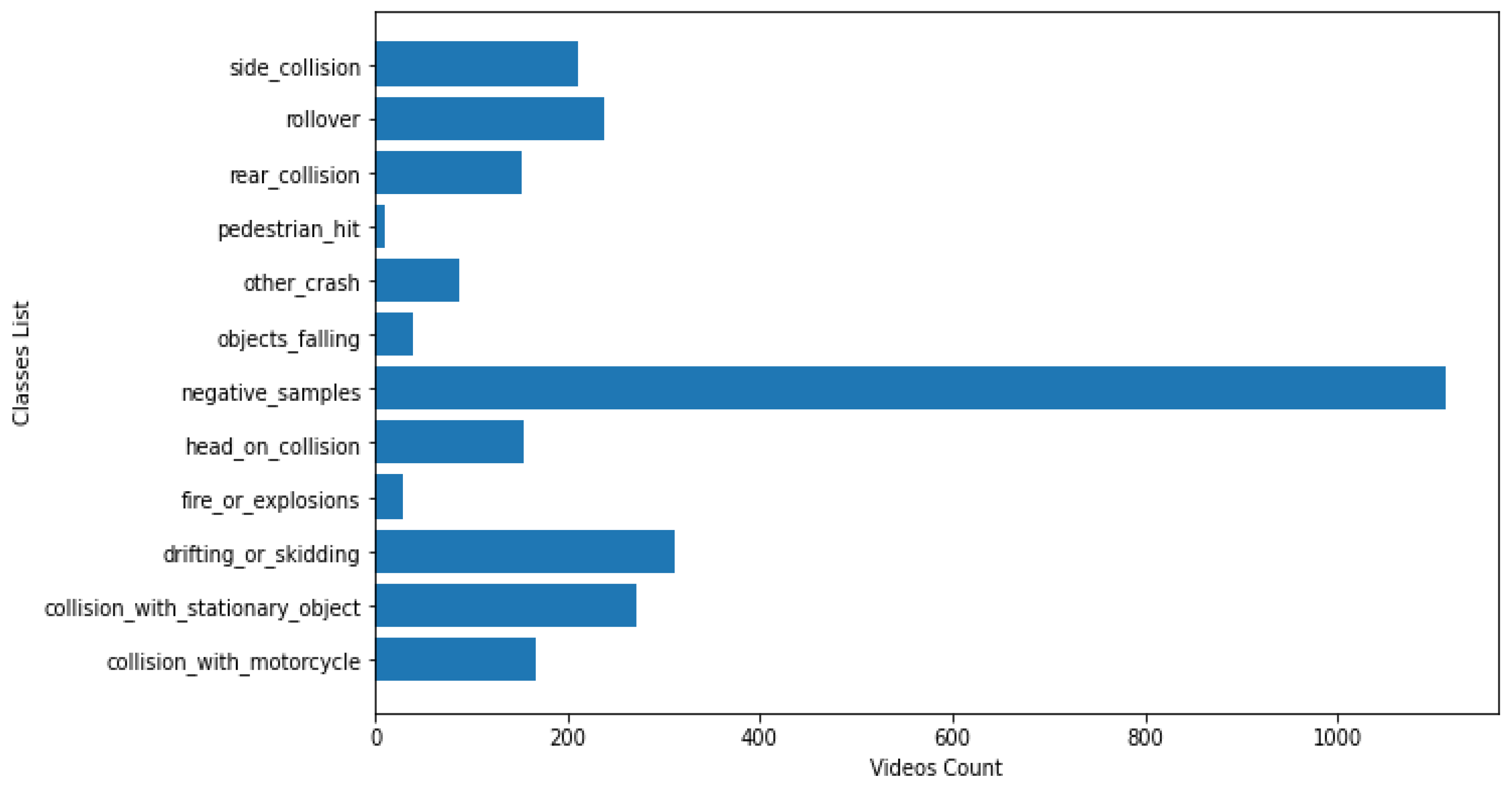
4.1.1. Highway Incidents Detection Dataset

The HWID12 [56] dataset consists of 12 total classes, 11 of which are different highway incidents, and one class for negative samples representing normal traffic. The range of the duration for each video is about 3 to 8 seconds on average. The dataset is specifically designed for road incident recognition. However, the dataset has a bias, and it needs curation which is shown in Figure 11. There are noticeable gaps in the number of samples in each class.

Accordingly, the different types of incidents were collected together and were classified as Abnormal. The dataset after the modification has two main classes, “Abnormal” with 1300 videos, which has different variations of accidents on the road, and “Normal” with 1110 videos, which has different sets of footage for typical traffic roads as shown in Figure 12. To our knowledge, we were the first to train and test this dataset after performing this modification to solve the class imbalance issue in the dataset.

4.1.2. Real Life Violence Situations Dataset

The RLVS dataset introduced by [57] benchmark consists of 2000 videos split into 1000 violent videos and 1000 non-violent videos as in Figure 13. The clips that were classified as violent and involved fights in various places and scenarios such as streets, prisons, and schools. The ones classified as non-violent show generic actions performed by humans, such as playing different sports and eating. Part of the RLVS dataset videos were manually captured, to make the dataset diverse in terms of the people appearing in the videos and the environment encapsulating them. Videos with long periods were shortened so that each video focused on the action itself.

4.1.3. Movie Fights and Hockey Fights Datasets

Movie Fights, and Hockey Fights [58] datasets were both proposed by the same authors, to test fight detection algorithms on various scenarios. The Movie Fights dataset contains 200 videos only, 100 per category from different action movies. While the Hockey Fights dataset contained 1000 videos, 500 per category, the videos contained fights between hockey players in the national hockey league in the USA. A sample from both datasets is shown below in Figure 14.

4.1.4. Datasets Observations and Analysis

In this section, an overview showing some information about the datasets used in the model development is shown in

Table 3. Overview about the datasets used.

Dataset	Number of Videos	Number of Normal Videos	Number of Abnormal Videos	Duration (s)	Resolution	FPS
RLVS	2000	1000	1000	3–7	High	10.5–37
HWID	2410	1110	1300	3–8	High	30
Hockey Fights	1000	500	500	1.6–1.96	Low	25
Movie Fights	200	100	100	1.66–2.04	Low	25–30

. For each dataset, the total number of videos, and the number of videos per class is shown. The range of duration and FPS for the videos in the datasets along with resolution description are also shown.

In Table 3, it is noticed that RLVS and HWID are the highest quality datasets that could be used for model development. These two have a larger duration range for each video, which means a wider coverage for the action. They also have a higher number of video samples to train and test on, and high resolution. Hockey and Movie Fights datasets suffer in every aspect, but they are covered here for comparison purposes later on. The two datasets Movies and Hockey Fights have a very limited amount of scenarios and are small in size, especially the Movie Fights dataset. Accordingly, we do not recommend working on those two datasets while making a model for a general-purpose application like a surveillance application for example.

4.2. Training Environment and Tools Used

The results were obtained after training on a GPU NVIDIA GeForce GTX 1070, with Intel CPU core i7 on a Windows 10 OS. The neural network architecture was programmed with computer vision and deep learning libraries like Tensorflow [59], OpenCV [60], and PyWavelets [61]. Within the different model proposals, the number of epochs is set to 50, the batch size is set to eight, and the input size is $100\times 100\times 3$. The HWID data was separated into training, and test data with a ratio of 70:30. The training data during the training process is further separated into training and validation with a ratio of 80:20. The movies and hockey data were separated with a ratio of 80:20, whereas the movies and hockey were further separated with 80:20 into training and validation. For RLVS, the training data was separated with a ratio of 90:10 in both separations. The optimizer used for the training process is the SGD with a learning rate of 1 × 10${}^{-4}$ and momentum of 0.9. The weight initialization is performed using He initialization [62] for all convolution weights and neurons in all architectures.

4.3. Evaluation Metrics and Methods Used

There are several evaluation metrics used for comparing the performance of classification models. One of the popular methods used is the construction of a confusion matrix. The matrix is a table with four different combinations of predicted and actual values. We also use the accuracy measure that obtains the number of samples in $TP$, $TN$, $FP$, and $FN$, which is a widely used metric when it comes to classification problems in deep learning. It evaluates if our model is trained well enough to be able to generalize on new test data. These four values were also used to measure precision, recall, and F1-score.

For the evaluation methods used, as shown in Figure 15, the holdout method is tried at first, to confirm the model’s performance a K-fold cross-validation is performed. The K-fold cross-validation is performed with five data splits, each split being stratified, meaning that each split is balanced, as each class has the same number of samples. Also, the resulting splits were obtained by randomized shuffling to make sure that each split was different from the other. The random state variable was also set to a different number other than the holdout to make sure that the obtained five splits are different from the holdout split.

4.4. Models Evaluation

Our experiments are divided into two stages which involve evaluating the proposed models twice. The first time the standard holdout technique is used by dividing the data into train-validation-test, and the second time the models are evaluated again using K-fold cross validation. The experiments are performed across all four datasets to confirm the proposed model’s performance.

4.4.1. Evaluating Different Proposed ISCA Blocks by Holdout Method

In this section, a comparison will be held among the four proposed wavelet blocks on top of the architecture. To ensure a fair comparison between the models, all experiments were performed using the same architecture of MobileNetV2, ConvLSTM, and fully connected neurons, under the same training settings, and same input properties.

During the training process, callbacks were used to monitor the performance of the model in a training session. Specifically, the early stopping and reducing learning rate on plateau from the Keras API were used. Early stopping stops the model training if the model performance in terms of validation loss is not improved after a certain patience measure—in our experiments, this was set to seven. As seen from Figure 16, each wavelet block had a different effect on the model, since each one started at a different accuracy and loss level. The DTCWT showed higher performance than DWT, which is expected since DTCWT shows less shift variance and more directional selectivity than the critically downsampled DWT, which means more information is exposed for the model to extract information from. The DWT showed the worst performance due to the above-mentioned reasons, and the $HH$ component contains noise despite the thresholding applied, which suggests the need for trying different thresholding techniques. DMWT also performed better than DWT, since multiple scaling and wavelet functions are used, but still lower than DTCWT.

The MultiWave shows the best performance of the wavelet blocks and has smoothed curves, which returns to the fact that the separate three channels exhibit different kinds of information, that still perfectly align with each other. The first two channels are basically analysis by synthesis processes generated from DWT and DMWT and the last channel can be considered as a data augmentation from the original image, except that there is no alteration to the information of the original image but rather a different re-arrangement to it, to focus on high frequency parts of the image, while preserving spatial information in the other two channels.

While training on the HWID, it can be noticed in Figure 17 that the Keras API stopped the training at 15 epochs. It was also noticed that the same performance was shown for the different inputs but all of them had smoother curves than those shown on RLVS, which returns to the high quality of the videos of the dataset, which in turn makes the predictions more consistent.

Furthermore, confusion matrices (CM) for each wavelet block are generated for the RLVS and HWID datasets as shown in

Table 4. Confusion matrices of different ISCA blocks on RLVS.

ISCA Block Type	TP	FP	FN	TN
DWT	85	14	6	95
DMWT	91	8	10	91
DTCWT	92	7	5	96
MultiWave	96	3	5	96

and

Table 5. Confusion matrices of different ISCA blocks on HWID.

ISCA Block Type	TP	FP	FN	TN
DWT	320	15	18	370
DMWT	331	4	19	369
DTCWT	326	9	9	379
MultiWave	387	9	4	323

.

From the confusion matrices generated, it can be noticed that the MultiWave ISCA block shows the best performance, as the total number of miss-classified videos ($FP$ and $FN$) is noticeably smaller than its other counterparts. The proposed model with MultiWave accomplished the highest accuracy when tested on both datasets. Now, in Figure 18, the validation accuracy and loss for the Hockey Fights and Movie Fights datasets are shown for the different ISCA blocks. For the Hockey and Movie Fights datasets, all models behaved just like RLVS in terms of not having smooth curves. In the movie’s accuracy graph, it is noticed that the DTCWT had lower accuracy than DWT, which shows a clear contradiction to what is supposed to happen. It is believed that returns to the small size of the dataset which make it not very reliable. That means DTCWT would need more training samples to obtain the expected result. All the models exhibit a clear ability to train and learn, as their validation accuracy is continuously increasing and the validation loss is continuously decreasing. In

Table 6. Confusion matrices of different ISCA blocks on hockey.

ISCA Block Type	TP	FP	FN	TN
DWT	87	9	8	96
DMWT	95	5	12	88
DTCWT	91	5	11	93
MultiWave	88	8	8	96

and

Table 7. Confusion matrices of different ISCA blocks on movies.

ISCA Block Type	TP	FP	FN	TN
DWT	18	2	0	20
DMWT	19	1	0	20
DTCWT	19	1	0	20
MultiWave	20	0	0	20

, the confusion matrices are shown for the Hockey and Movie Fights datasets.

The same as RLVS and HWID, the models showed a great learning capability where both ($TP$ and $TN$) are noticeably larger compared to ($FP$ and $FN$) on the test samples of both datasets. In

Table 8. Performance of different ISCA blocks on different datasets.

ISCA Block Type	RLVS	HWID	Hockey Fights	Movie Fights
DWT	90.00	95.44	91.50	95
DMWT	91.00	97.00	91.50	97.50
DTCWT	94	97.51	92.00	97.50
MultiWave	96	98.20	92.00	100

, all the test accuracies are shown for all models across the different datasets used. From all datasets, the DWT in particular had the lowest test accuracy compared to the other blocks. Sometimes the margin is not large when compared to DMWT, but compared to DTCWT and MultiWave, the difference is large.

4.4.2. Evaluating Different Proposed ISCA Blocks by Cross-Validation on RLVS Dataset

The cross-validation was performed with the same train/test data split ratio, and all the training settings as in the holdout method. As shown in

Table 9. Performance of Different ISCA Blocks on different RLVS data splits.

ISCA Block Type	Split 1	Split 2	Split 3	Split 4	Split 5	Mean Accuracy
DWT	90.5	91.5	88.4	87	91	89.73
DMWT	89	92.5	91	91	94.5	91.50
DTCWT	93	96	92	89.5	94.5	93.16
MultiWave	92	94.5	92	93	92	93.25

, the mean accuracy calculated here combines both the cross-validation splits and the holdout split.

It is noticed that the DWT block offered a lower accuracy compared to the other blocks. Meanwhile, both DMWT and DTCWT had better performance but they were inconsistent with each split. The overall mean accuracy for both DTCWT and MultiWave is close but it is worth taking into consideration that the MultiWave block is less computationally expensive since it works on $100\times 100$, unlike DTCWT which works on $200\times 200$. Figure 19 shows the validation accuracy of all four proposed blocks across the different data splits.

It is noticed from the figure that the performance of the models across the different splits is similar to the holdout in terms of the number of epochs and the rigid curves. The DMWT on split four had the longest training time out of all the scenarios. In

Table 10. Model evaluation of the proposed ISCA blocks on RLVS.

Metric	DWT	DMWT	DTCWT	MultiWave
Precision	0.910	0.920	0.934	0.930
Recall	0.918	0.916	0.932	0.930
F1-score	0.916	0.914	0.928	0.930

, the average precision, recall, and F1-score were calculated for all the proposed ISCA blocks across all the data splits.

4.4.3. Evaluating Different Proposed ISCA Blocks by Cross-Validation on HWID Dataset

In this section, the same settings are applied again but on the curated HWID dataset as shown in

Table 11. Performance of different ISCA blocks on different HWID data splits.

ISCA Block Type	Split 1	Split 2	Split 3	Split 4	Split 5	Mean Accuracy
DWT	95.44	97.00	97.09	97.37	97.90	96.70
DMWT	95.15	94.88	96.82	96.40	97.79	96.34
DTCWT	98.06	96.95	96.96	95.71	97.79	97.16
MultiWave	96.82	97.65	96.54	97.37	96.69	97.21

. The mean accuracy calculated here combines both the cross-validation splits and the holdout split.

It is noticed from this table that the accuracy obtained from all variations is high, which means the model is performing well on this dataset. They are also very close to each other unlike what happened in RLVS, which might return to the high-quality videos in the dataset. In Figure 20, the validation accuracy obtained is shown from all block variations across the different data splits.

It is noticed here that smoother curves are obtained like the holdout method, but the models trained for a longer amount of time. The DWT on split four had the longest training out of all the scenarios. In

Table 12. Model evaluation of the proposed ISCA blocks on HWID.

Metric	DWT	DMWT	DTCWT	MultiWave
Precision	0.968	0.962	0.972	0.972
Recall	0.968	0.962	0.972	0.972
F1-score	0.968	0.962	0.972	0.972

, the average precision, recall, and F1-score were calculated for all the proposed ISCA blocks across all the data splits.

4.4.4. Evaluating Different Proposed ISCA Blocks by Cross-Validation on Hockey Fight Dataset

In this section, the same training settings are applied once again but on the Hockey Fights dataset as shown in

Table 13. Performance of different ISCA blocks on different hockey fights data splits.

ISCA Block Type	Split 1	Split 2	Split 3	Split 4	Split 5	Mean Accuracy
DWT	91.50	89.90	93.00	94.50	90.50	91.70
DMWT	91.50	93.00	95.50	91.50	94.50	93.00
DTCWT	92.00	91.00	92.50	95.00	94.00	92.75
MultiWave	90.50	92.00	93.00	92.00	92.00	91.91

. The mean accuracy calculated here combines both the cross-validation splits and the holdout split.

From this table, it is noticed that the gap between both DWT and MultiWave is not high compared to the other datasets, while both DMWT and DTCWT outperform them. In Figure 21, the validation accuracy obtained across the different splits with all bock variations is shown.

From the curves shown, the performance of each block on this dataset during the training process varies from one to the other, implying that the dataset had a different effect when each process was applied to it. In

Table 14. Model evaluation of the proposed ISCA blocks on hockey fights.

Metric	DWT	DMWT	DTCWT	MultiWave
Precision	0.922	0.936	0.930	0.920
Recall	0.920	0.932	0.930	0.920
F1-score	0.916	0.928	0.928	0.918

, the average precision, recall, and F1-score were calculated for all the proposed ISCA blocks across all the data splits.

4.4.5. Evaluating Different Proposed ISCA Blocks by Cross-Validation on Movies Dataset

Lastly, in this section the same training settings are applied but on the Movie Fights dataset as shown in

Table 15. Performance of different ISCA blocks on different movie fights data splits.

ISCA Block Type	Split 1	Split 2	Split 3	Split 4	Split 5	Mean Accuracy
DWT	95.00	95.00	100.00	95.00	95.00	95.83
DMWT	97.50	95.00	100.00	97.50	100.00	98.00
DTCWT	97.50	92.50	95.00	97.50	95.00	95.83
MultiWave	97.50	92.50	100.00	100.00	95.00	97.50

. The mean accuracy calculated here combines both the cross-validation splits and the holdout split.

Due to the small size of this dataset, it is quite common for good models to achieve $100\%$ accuracy. It can be seen that on splits one and two, none of the models obtained $100\%$ accuracy but still achieved very high accuracies, unlike on splits three, four, and five. It is also noticed that DMWT and MultiWave had the highest accuracy. In Figure 22, the model validation accuracy is shown across different data splits for all four blocks.

From the curves displayed above, almost all the splits could reach a $100\%$ validation accuracy. The MultiWave performance seemed to start from a lower point than usual when used on split five but succeeded in bypassing the challenge to the $100\%$. In

Table 16. Model evaluation of the proposed ISCA blocks on movie fights.

Metric	DWT	DMWT	DTCWT	MultiWave
Precision	0.960	0.982	0.958	0.972
Recall	0.960	0.978	0.954	0.970
F1-score	0.960	0.978	0.952	0.970

, the average precision, recall, and F1-scores were calculated for all the proposed ISCA blocks across all the data splits.

4.4.6. Evaluating Inference Time of Different ISCA Blocks

In this section, a time analysis is performed on the different ISCA blocks in order to test which one of them can be used in a real-time case scenario. Each ISCA block is used with MobileNetV2 and ConvLSTM. This analysis is conducted over 100 inference runs, in order to obtain a somewhat close estimate of the model speed. The recorded data included the minimum and maximum inference times, along with the standard deviation and average inference time. This time analysis is shown in

Table 17. Time analysis of the wavelet-based ISCA blocks.

Block	Minimum Inference Time (ms)	Maximum Inference Time (ms)	Standard Deviation	Average Inference Time (ms)
DWT	82	101.66	3.62	88.19
DMWT	87.7	1371.27	137.78	108.97
DTCWT	88.7	2881.19	300.36	128.95
MultiWave	76	110.23	5.88	90.44

. As seen from the table, both DWT and MultiWave have better metrics to be considered in a real-time scenario than DMWT and DTCWT by a big margin.

4.4.7. Model Evaluation Discussion and Main Takeaways

In this section, a discussion is held in order to determine the strengths and weaknesses of each wavelet-based ISCA block in accordance with the previous experiments conducted. In the following

Table 18. Observations on the model evaluation.

Block	Reliable Training Performance	Reliable Generalization on Test Data	Suitability for Real-Time
DWT	Yes	No	Yes
DMWT	Yes	Yes	No
DTCWT	Yes	Yes	No
MultiWave	Yes	Yes	Yes

, we try to identify the main points, where a decision for that model can be made regarding its usability in a real-time case scenario. Each column in the table is considered a ’Yes’ or ’No’ question and is answered accordingly based on our observations from the training and testing runs using holdout and cross-validation experiments.

As one can see, all the blocks received a ’Yes’ for reliable performance during training, as the model validation accuracy increased steadily with each epoch, and the loss decreased with all datasets. While DWT stood out in the reliable generalization ability on test data, which is evident on the RLVS dataset, it had lower performance compared to others on some data splits. As for the suitability to run in real-time, only DWT and MultiWave blocks can work without time lags in real-time, however, the MultiWave is more reliable in terms of accuracy. In the holdout method, when the data is split into the training, validation, and test samples, this split could have a bias since there is no guarantee of randomness within the split even if the whole dataset is considered a random sample. To alleviate this bias, the test accuracy obtained from the different splits can be averaged which is precisely what the cross-validation does. There is also a difference between the holdout and cross-validation results obtained since the numbers are not the same, however, that difference is very small, which makes it safe to assume that the model does not overfit to a specific data split.

4.5. Ablation Study

In this section, an ablation study was conducted, where some parts of the model were removed and replaced with other components to find out how the performance obtained can be attributed to the model’s different constituent parts. Firstly, different input sizes and sequence lengths are tried to examine the effect of the input shape on the performance. Secondly, different spatial backbones are tried, to validate the performance of the MobileNetV2 with the wavelet-based ISCA block. Thirdly, different temporal units are tried with the ISCA block and examine the effect. All the experiments performed in this section were performed on the RLVS dataset.

4.5.1. Testing Different Input Sizes and Sequence Lengths

The first part of the ablation study starts with investigating the input shapes of the data to the model to determine the effect of such factors on the model performance. In

Table 19. Effect of the sequence length on the accuracy.

Sequence Length	Accuracy
4	92.50
8	93.50
12	94.50
16	96.00

, the effect of trying different sequence lengths is shown on the accuracy. It seems like the longer the sequence length, the higher the accuracy but the margin of the difference is not large.

In

Table 20. Effect of the input size on the accuracy.

Input Size	Accuracy
$50\times 50$	79.00
$70\times 70$	86.00
$100\times 100$	96.00

, different input sizes for the image data are tried to examine the effect on the accuracy. It is noticeable that the difference in the accuracy between the different input sizes is large compared to the shorter sequence lengths used, which indicates that the input size had more effect on the performance than the sequence length used.

4.5.2. Testing Different Spatial Backbones

In this part of the ablation study, we compare our choice of using MobileNetV2 based on our hypothesis with other CNN backbones to prove the effectiveness of our approach with the proposed ISCA blocks. The MultiWave block and ConvLSTM were used here along with different backbones as shown in

Table 21. Performance of MultiWave ISCA block and ConvLSTM with different CNN backbones.

Backbone	Backbone Inference Time (ms)	Total Model Parameters	Accuracy
ResNet-50 [63]	58.2	28,468,370	76
Inception-V3 [64]	42.2	26,683,442	89
DenseNet-121 [65]	77.1	9,558,866	94
EfficientNetB5 [66]	579.2	7,160,757	62
MobileNet-V2 [48]	25.9	5,369,170	96

.

From the table above, it is noticed that MobileNetV2 has the least amount of parameters and inference time while having the highest accuracy. That proves the effectiveness of the MultiWave ISCA block as intended. That returns us to the fact that the ISCA block exposes high frequencies directly to the CNN, so the CNN does not have to work on extracting those features as much as it would usually. When such high frequencies go through many layers that are not needed, it has a reverse effect and degrades the features in the final layers resulting in such low accuracies. Also, MobileNetV2 has fewer pooling layers than other backbones, which makes it to be the best choice to work with the ISCA block.

4.5.3. Testing Different Temporal Units

In this part of the ablation study, different temporal units are used and compared against each other while using the MultiWave ISCA block and MobileNetV2 on the RLVS dataset as shown in

Table 22. Performance of MultiWave ISCA block and MobileNetV2 with different temporal units.

Temporal Unit	Total Model Parameters	Accuracy
GRU [67]	2,533,570	94
LSTM [68]	2,619,458	94
Bi-LSTM [69]	2,980,162	92
ConvLSTM [49]	5,369,170	96

.

From the table mentioned, the ConvLSTM unit gave the best performance as expected, due to its ability to extract local spatiotemporal features as discussed in the methods section. The GRU and LSTM units gave the same performance, lower than ConvLSTM, but near to be good enough to be considered as an alternative to work on an edge unit for example, due to the significant decrease in the number of parameters, which means higher inference speed.

4.6. Comparison with Other Methods

In this section, a comparison will be held between the proposed best-performing models; the one that uses MultiWave ISCA block, against other different recent models on RLVS, Movie Fights, and Hockey Fight datasets. The HWID dataset is left out of the comparison due to the absence of other models that tested on it the same way that was performed. Starting with RLVS, the following

Table 23. Comparison with other methods on the RLVS dataset.

Method	Accuracy	Efficiency
2D-Convolution + LSTM [29]	92%	≈4.6 m
ViolenceNet Pseudo-Optical Flow [27]	94.10%	$4.5$ m
Keyframe-based ResNet18 [70]	94.60%	≈11.6 m
U-NET + LSTM [71]	94%	≈4 m
VGG-16 + LSTM [57]	88.2%	≈140 m
MobileNetV2 [72]	94%	≈3.2 m
Motion Features + Inception-ResNet [73]	86.78%	≈59.6 m
Proposed Model	96%	$O\left(N\right)$ for wavelet transform, $5.3$ m

shows a comparison between the proposed best-performing model and other approaches. It is shown how our proposed model can achieve a competitive performance with the state-of-the-art while optimizing the number of parameters.

In

Table 24. Comparison with other methods on the Movie Fights and Hockey Fights datasets.

Method	Movies	Hockey	Efficiency
ViF + SVM [74]	-	82.90%	Fast, but not Robust.
ConvLSTM [75]	95%	91%	≈62.5 k
3D-CNN [76]	-	96%	≈78 m
Multistream-VGG16 [77]	100%	89.10%	≈138 m $\times 4$
ResNet50 + ConvLSTM [78]	88.74%	83.19%	≈24.7 m
Radon Transform [79]	98%	90.01%	Fast, but not Robust.
Motion Features + Inception-ResNetV2 [73]	100%	93.33%	≈59.6 m
Proposed Model	99.5%	92%	$O\left(N\right)$ for wavelet transform, $5.3$ m

, the comparison is held with other approaches, where the classical approaches do not have learnable parameters; a description is provided for the approach. In our approach, the time complexity in terms of big-o-notation is provided with the non-learnable part of the model, and then the number of parameters is provided for the rest of the model. It is noticed in the two tables that the proposed model outperforms the other models either accuracy-wise, efficiency-wise in terms of a number of parameters, or both. When compared with other methods on both datasets, the proposed model had $4.05\%$ more accuracy on average for the RLVS dataset, while on movies the proposed model had $6.08\%$ more accuracy on average, and finally on hockey it had $4.782\%$ more accuracy on average. As for the efficiency, the proposed model had on average $139.1$ m fewer parameters than the others.

5. Conclusions and Future Work

In this paper, the problem of anomalous actions that are captured by cameras is tackled. Anomalous actions are defined in the sense of human violence or road accidents. For that purpose, a novel channel-wise augmentation technique using different types of wavelet transforms is introduced on top of a spatiotemporal architecture. The hypothesis states that a CNN model focuses on the high frequency components when extracting features for classification, hence different types of wavelet transform are used and compared against each other in a detailed ablation study. All experiments were conducted using the same MobileNetV2 model with transfer learning for spatial feature extraction and ConvLSTM for temporal feature extraction. The same input dimensions and training settings were used during the comparison. The training and testing were performed on four public datasets for anomalous actions, namely RLVS, HWID, Movie Fights, and Hockey Fights. Several ISCA blocks are proposed, so to confirm their performance, two evaluation methods were applied; the holdout and cross-validation techniques. After testing, the MultiWave ISCA block achieved the best accuracies of $96\%$, $98.20\%$, $92\%$, and $99.5\%$ on RLVS, HWID, Hockey Fights, and Movie Fights, respectively.

Further analysis was performed in the form of cross-validation on all datasets to confirm the performance of the different blocks. The MultiWave block did not have the highest accuracy across all the datasets like in the holdout method. However, after performing the time analysis in real time, the MultiWave and DWT had better statistics than DTCWT and DMWT. This work proves the positive effect of letting a classification model extract wavelet-based features. Also, after performing the comparison with other methods, the model offers a competitive performance in terms of accuracy and efficiency.

For future work, other wavelet transform techniques like fully separable wavelet transform [80] and stationary wavelet transform should be tried along with different thresholding techniques like Bivariate CWT [81] to filter out the noise. Extending on the current violence datasets, to include different illuminations, to make the model robust in such scenarios. Also, the model can be extended for multi-classification to classify several abnormal actions. However, a diverse and large multi-class dataset needs to be gathered for abnormal action recognition. The current multi-class datasets suffer from a few shortcomings, which include bias towards some classes in the datasets, and the videos in each class do not focus on the intended action which affects the learning process of the model during training. A large multi-class dataset opens the door for research in making larger models to train on these datasets with higher performance, the current state-of-the-art focuses on using video transformers in different combinations to classify videos, however, the main issue is that these models contain a very large number of trainable parameters while offering little performance improvement compared to traditional deep CNNs, which limits them for deployment on edge devices.

References

1. Shoukry, N.; Abd El Ghany, M.A.; Salem, M.A.M. Multi-Modal Long-Term Person Re-Identification Using Physical Soft Bio-Metrics and Body Figure. Appl. Sci. 2022, 12, 2835. [Google Scholar] [CrossRef]
2. Fahmy, M.; Fahmy, O. A new image denoising technique using orthogonal complex wavelets. In Proceedings of the 2018 35th National Radio Science Conference (NRSC), Cairo, Egypt, 20–22 March 2018; pp. 223–230. [Google Scholar] [CrossRef]
3. Fahmy, G.; Fahmy, O.; Fahmy, M. Fast Enhanced DWT based Video Micro Movement Magnification. In Proceedings of the 2019 IEEE International Symposium on Signal Processing and Information Technology (ISSPIT), Ajman, United Arab Emirates, 10–12 December 2019; pp. 1–6. [Google Scholar] [CrossRef]
4. Alaba, S.; Ball, J. WCNN3D: Wavelet Convolutional Neural Network-Based 3D Object Detection for Autonomous Driving. Sensors 2022, 22, 7010. [Google Scholar] [CrossRef] [PubMed]
5. Yao, T.; Pan, Y.; Li, Y.; Ngo, C.W.; Mei, T. Wave-ViT: Unifying Wavelet and Transformers for Visual Representation Learning. In Proceedings of the Computer Vision—ECCV 2022, Tel Aviv, Israel, 23–27 October 2022; pp. 328–345. [Google Scholar] [CrossRef]
6. Zhao, X.; Huang, P.; Shu, X. Wavelet-Attention CNN for image classification. Multimed. Syst. 2022, 28, 915–924. [Google Scholar] [CrossRef]
7. Williams, T.; Li, R. Wavelet Pooling for Convolutional Neural Networks. In Proceedings of the International Conference on Learning Representations, Vancouver, BC, Canada, 30 April–3 May 2018. [Google Scholar]
8. Fujieda, S.; Takayama, K.; Hachisuka, T. Wavelet Convolutional Neural Networks for Texture Classification. arXiv 2017, arXiv:1707.07394. [Google Scholar]
9. Huang, H.; He, R.; Sun, Z.; Tan, T. Wavelet-SRNet: A Wavelet-Based CNN for Multi-scale Face Super Resolution. In Proceedings of the 2017 IEEE International Conference on Computer Vision (ICCV), Venice, Italy, 22–29 October 2017; pp. 1698–1706. [Google Scholar] [CrossRef]
10. Ridha Ilyas, B.; Beladgham, M.; Merit, K.; Taleb Ahmed, A. Improved Facial Expression Recognition Based on DWT Feature for Deep CNN. Electronics 2019, 8, 324. [Google Scholar] [CrossRef]
11. Youyi, J.; Xiao, L. A Method for Face Recognition Based on Wavelet Neural Network. In Proceedings of the 2010 Second WRI Global Congress on Intelligent Systems, Wuhan, China, 16–17 December 2010; Volume 3, pp. 133–136. [Google Scholar] [CrossRef]
12. Liu, P.; Zhang, H.; Zhang, K.; Lin, L.; Zuo, W. Multi-level Wavelet-CNN for Image Restoration. In Proceedings of the 2018 IEEE/CVF Conference on Computer Vision and Pattern Recognition Workshops (CVPRW), Salt Lake City, UT, USA, 18–22 June 2018; pp. 886–88609. [Google Scholar] [CrossRef]
13. Wang, H.; Wu, X.; Huang, Z.; Xing, E. High-Frequency Component Helps Explain the Generalization of Convolutional Neural Networks. In Proceedings of the 2020 IEEE/CVF Conference on Computer Vision and Pattern Recognition (CVPR), Seattle, WA, USA, 13–19 June 2020; pp. 8681–8691. [Google Scholar] [CrossRef]
14. Lahiri, D.; Dhiman, C.; Vishwakarma, D. Abnormal human action recognition using average energy images. In Proceedings of the In 2017 Conference on Information and Communication Technology (CICT), Gwalior, India, 3–5 November 2017; pp. 1–5. [Google Scholar] [CrossRef]
15. Dhiman, C.; Vishwakarma, D. A Robust Framework for Abnormal Human Action Recognition using R-Transform and Zernike Moments in Depth Videos. IEEE Sens. J. 2019, 19, 5195–5203. [Google Scholar] [CrossRef]
16. Vishwakarma, D.; Dhiman, C. A unified model for human activity recognition using spatial distribution of gradients and difference of Gaussian kernel. Vis. Comput. 2019, 35, 1–19. [Google Scholar] [CrossRef]
17. Ayman, O.; Marzouk, N.; Atef, E.; Salem, M.; Salem, M.A.M.M. Abnormal Action Detection In Video Surveillance. In Proceedings of the 9th IEEE International Conference on Intelligent Computing and Information Systems, Cairo, Egypt, 8–9 December 2020. [Google Scholar] [CrossRef]
18. Tay, N.; Connie, T.; Ong, T.S.; Goh, K.; Teh, P.S. A Robust Abnormal Behavior Detection Method Using Convolutional Neural Network. In Proceedings of the 5th ICCST 2018, Kota Kinabalu, Malaysia, 29–30 August 2018; pp. 37–47. [Google Scholar] [CrossRef]
19. Arunnehru, J.; Chamundeeswari, G.; Bharathi, S. Human Action Recognition using 3D Convolutional Neural Networks with 3D Motion Cuboids in Surveillance Videos. Procedia Comput. Sci. 2018, 133, 471–477. [Google Scholar] [CrossRef]
20. Vršková, R.; Hudec, R.; Kamencay, P.; Sykora, P. Human Activity Classification Using the 3DCNN Architecture. Appl. Sci. 2022, 12, 931. [Google Scholar] [CrossRef]
21. Dhiman, C.; Vishwakarma, D.; Agarwal, P. Part-wise Spatio-temporal Attention Driven CNN-based 3D Human Action Recognition. ACM Trans. Multimed. Comput. Commun. Appl. 2021, 17, 1–24. [Google Scholar] [CrossRef]
22. Chen, B.; Tang, H.; Zhang, Z.; Tong, G.; Li, B. Video-based action recognition using spurious-3D residual attention networks. IET Image Process. 2022, 16, 3097–3111. [Google Scholar] [CrossRef]
23. Qian, H.; Zhou, X.; Zheng, M. Abnormal Behavior Detection and Recognition Method Based on Improved ResNet Model. Comput. Mater. Contin. 2020, 65, 2153–2167. [Google Scholar] [CrossRef]
24. Magdy, M.; Fakhr, M.; Maghraby, F. Violence 4D: Violence detection in surveillance using 4D convolutional neural networks. IET Comput. Vision 2022, 17, 282–294. [Google Scholar] [CrossRef]
25. Vršková, R.; Hudec, R.; Kamencay, P.; Sykora, P. A New Approach for Abnormal Human Activities Recognition Based on ConvLSTM Architecture. Sensors 2022, 22, 2946. [Google Scholar] [CrossRef] [PubMed]
26. Vijeikis, R.; Raudonis, V.; Dervinis, G. Efficient Violence Detection in Surveillance. Sensors 2022, 22, 2216. [Google Scholar] [CrossRef] [PubMed]
27. Rendón-Segador, F.; Alvarez-Garcia, J.; Enriquez, F.; Deniz, O. ViolenceNet: Dense Multi-Head Self-Attention with Bidirectional Convolutional LSTM for Detecting Violence. Electronics 2021, 10, 1601. [Google Scholar] [CrossRef]
28. Kalfaoglu, E.; Kalkan, S.; Alatan, A. Late Temporal Modeling in 3D CNN Architectures with BERT for Action Recognition. In Proceedings of the Computer Vision–ECCV 2020 Workshops, Glasgow, UK, 23–28 August 2020. [Google Scholar]
29. Moaaz, M.; Mohamed, E. Violence Detection In Surveillance Videos Using Deep Learning. Inform. Bull. Fac. Comput. Artif. Intell. 2020, 2, 6. [Google Scholar] [CrossRef]
30. Ullah, A.; Ahmad, J.; Muhammad, K.; Sajjad, M.; Baik, S. Action Recognition in Video Sequences using Deep Bi-directional LSTM with CNN Features. IEEE Access 2017, 6, 1155–1166. [Google Scholar] [CrossRef]
31. Chen, W.; Zheng, F.; Gao, S.; Hu, K. An LSTM with Differential Structure and Its Application in Action Recognition. Math. Probl. Eng. 2022, 2022, 7316396. [Google Scholar] [CrossRef]
32. Al-berry, M.; Salem, M.A.M.M.; Ebied, H.; Hussein, A.; Tolba, M. Action Recognition Using Stationary Wavelet-Based Motion Images. In Intelligent Systems’ 2014, Proceedings of the 7th IEEE International Conference Intelligent Systems IS’2014, Warsaw, Poland, 24--26 September 2014; Springer International Publishing: Berlin/Heidelberg, Germany, 2014; Volume 323, pp. 743–753. [Google Scholar] [CrossRef]
33. Al-berry, M.; Salem, M.A.M.M.; Ebied, H.; Hussein, A.; Tolba, M. Action Classification Using Weighted Directional Wavelet LBP Histograms. In Proceedings of the 1st International Conference on Advanced Intelligent System and Informatics (AISI2015), Beni Suef, Egypt, 28–30 November 2015. [Google Scholar] [CrossRef]
34. Chatterjee, R.; Halder, R. Discrete Wavelet Transform for CNN-BiLSTM-based Violence Detection. In Proceedings of the International Conference on Emerging Trends and Advances in Electrical Engineering and Renewable Energy, Bhubaneswar, India, 5–6 March 2020; Springer Nature: Singapore, 2020. [Google Scholar]
35. Nedorubova, A.; Kadyrova, A.; Khlyupin, A. Human Activity Recognition using Continuous Wavelet Transform and Convolutional Neural Networks. arXiv 2021, arXiv:2106.12666. [Google Scholar] [CrossRef]
36. Neimark, D.; Bar, O.; Zohar, M.; Asselmann, D. Video Transformer Network. In Proceedings of the 2021 IEEE/CVF International Conference on Computer Vision Workshops (ICCVW), Montreal, BC, Canada, 11–17 October2021; pp. 3156–3165. [Google Scholar] [CrossRef]
37. Girdhar, R.; Carreira, J.; Doersch, C.; Zisserman, A. Video Action Transformer Network. In Proceedings of the IEEE/CVF Conference on Computer Vision and Pattern Recognition (CVPR), Long Beach, CA, USA, 15–20 June 2019. [Google Scholar]
38. Sargano, A.B.; Angelov, P.; Habib, Z. A Comprehensive Review on Handcrafted and Learning-Based Action Representation Approaches for Human Activity Recognition. Appl. Sci. 2017, 7, 110. [Google Scholar] [CrossRef]
39. Mumtaz, N.; Ejaz, N.; Habib, S.; Mohsin, S.M.; Tiwari, P.; Band, S.S.; Kumar, N. An overview of violence detection techniques: Current challenges and future directions. Artif. Intell. Rev. 2023, 56, 4641–4666. [Google Scholar] [CrossRef]
40. Malik, Z.; Shapiai, M.I.B. Human action interpretation using convolutional neural network: A survey. Mach. Vis. Appl. 2022, 33, 37. [Google Scholar] [CrossRef]
41. Ulhaq, A.; Akhtar, N.; Pogrebna, G.; Mian, A. Vision Transformers for Action Recognition: A Survey. arXiv 2022, arXiv:2209.05700. [Google Scholar]
42. Debnath, L.; Antoine, J.P. Wavelet Transforms and Their Applications. Phys. Today 2003, 56, 68. [Google Scholar] [CrossRef]
43. Skodras, N. Discrete Wavelet Transform: An Introduction; Hellenic Open University Technical Report; Hellenic Open University: Patras, Greece, 2003; Volume 2, pp. 1–26. [Google Scholar]
44. Selesnick, I.; Baraniuk, R.; Kingsbury, N. The dual-tree complex wavelet transform. Signal Process. Mag. IEEE 2005, 22, 123–151. [Google Scholar] [CrossRef]
45. Geronimo, J.; Hardin, D.; Massopust, P. Fractal Functions and Wavelet Expansion Based on Several Scaling Functions. J. Approx. Theory 1994, 78, 373–401. [Google Scholar] [CrossRef]
46. Zhuang, F.; Qi, Z.; Duan, K.; Xi, D.; Zhu, Y.; Zhu, H.; Xiong, H.; He, Q. A Comprehensive Survey on Transfer Learning. Proc. IEEE 2020, 109, 43–76. [Google Scholar] [CrossRef]
47. Deng, J.; Dong, W.; Socher, R.; Li, L.J.; Li, K.; Li, F.F. ImageNet: A Large-Scale Hierarchical Image Database. In Proceedings of the 2009 IEEE Conference on Computer Vision and Pattern Recognition, Miami, FL, USA, 20–25 June 2009; pp. 248–255. [Google Scholar] [CrossRef]
48. Sandler, M.; Howard, A.; Zhu, M.; Zhmoginov, A.; Chen, L.C. Mobilenetv2: Inverted residuals and linear bottlenecks. In Proceedings of the IEEE Conference on Computer Vision and Pattern Recognition, Salt Lake City, UT, USA, 18–23 June 2018; pp. 4510–4520. [Google Scholar]
49. Shi, X.; Chen, Z.; Wang, H.; Yeung, D.Y.; Wong, W.k.; Woo, W.c. Convolutional LSTM Network: A Machine Learning Approach for Precipitation Nowcasting. arXiv 2015, arXiv:1506.04214. [Google Scholar] [CrossRef]
50. Sernani, P.; Falcionelli, N.; Tomassini, S.; Contardo, P.; Dragoni, A.F. Deep Learning for Automatic Violence Detection: Tests on the AIRTLab Dataset. IEEE Access 2021, 9, 160580–160595. [Google Scholar] [CrossRef]
51. Chen, S.; Xu, X.; Zhang, Y.; Shao, D.; Zhang, S.; Zeng, M. Two-stream convolutional LSTM for precipitation nowcasting. Neural Comput. Appl. 2022, 34, 13281–13290. [Google Scholar] [CrossRef]
52. Shibuya, E.; Hotta, K. Cell image segmentation by using feedback and convolutional LSTM. Vis. Comput. 2021, 38, 3791–3801. [Google Scholar] [CrossRef]
53. Wei, H.; Li, K.; Li, H.; Lyu, Y.; Hu, X. Detecting Video Anomaly with a Stacked Convolutional LSTM Framework. In Proceedings of the International Conference on Computer Vision Systems, Thessaloniki, Greece, 23–25 September 2019; Springer International Publishing: Cham, Switzerland, 2019; pp. 330–342. [Google Scholar] [CrossRef]
54. Donoho, D. De-noising by soft-thresholding. IEEE Trans. Inf. Theory 1995, 41, 613–627. [Google Scholar] [CrossRef]
55. Donoho, D.L.; Johnstone, I.M. Adapting to Unknown Smoothness via Wavelet Shrinkage. J. Am. Stat. Assoc. 1995, 90, 1200–1224. [Google Scholar] [CrossRef]
56. Kezebou, L.; Oludare, V.; Panetta, K.; Intriligator, J.; Agaian, S. Highway accident detection and classification from live traffic surveillance cameras: A comprehensive dataset and video action recognition benchmarking. In Proceedings of the Multimodal Image Exploitation and Learning, Orlando, FL, USA, 3 April–12 June 2022; SPIE: Bellingham, WA, USA, 2022; Volume 12100, pp. 240–250. [Google Scholar]
57. Soliman, M.M.; Kamal, M.H.; El-Massih Nashed, M.A.; Mostafa, Y.M.; Chawky, B.S.; Khattab, D. Violence Recognition from Videos using Deep Learning Techniques. In Proceedings of the 2019 Ninth International Conference on Intelligent Computing and Information Systems (ICICIS), Cairo, Egypt, 8–10 December 2019; pp. 80–85. [Google Scholar] [CrossRef]
58. Nievas, E.B.; Suarez, O.D.; Garcia, G.B.; Sukthankar, R. Hockey Fight Detection Dataset. In Computer Analysis of Images and Patterns; Springer: Berlin/Heidelberg, Germany, 2011; pp. 332–339. [Google Scholar]
59. Abadi, M.; Agarwal, A.; Barham, P.; Brevdo, E.; Chen, Z.; Citro, C.; Corrado, G.S.; Davis, A.; Dean, J.; Devin, M.; et al. TensorFlow: Large-Scale Machine Learning on Heterogeneous Systems. arXiv 2015, arXiv:1603.04467. Available online: tensorflow.org (accessed on 2 January 2024).
60. Bradski, G. The OpenCV Library. Dr. Dobb’S J. Softw. Tools 2000, 25, 120–123. [Google Scholar]
61. Lee, G.R.; Gommers, R.; Waselewski, F.; Wohlfahrt, K.; Leary, A. PyWavelets: A Python package for wavelet analysis. J. Open Source Softw. 2019, 4, 1237. [Google Scholar] [CrossRef]
62. He, K.; Zhang, X.; Ren, S.; Sun, J. Delving Deep into Rectifiers: Surpassing Human-Level Performance on ImageNet Classification. In Proceedings of the 2015 IEEE International Conference on Computer Vision (ICCV), Santiago, Chile, 7–13 December 2015; pp. 1026–1034. [Google Scholar] [CrossRef]
63. He, K.; Zhang, X.; Ren, S.; Sun, J. Deep Residual Learning for Image Recognition. In Proceedings of the 2016 IEEE Conference on Computer Vision and Pattern Recognition (CVPR), Las Vegas, NV, USA, 27–30 June2016; pp. 770–778. [Google Scholar] [CrossRef]
64. Szegedy, C.; Liu, W.; Jia, Y.; Sermanet, P.; Reed, S.; Anguelov, D.; Erhan, D.; Vanhoucke, V.; Rabinovich, A. Going deeper with convolutions. In Proceedings of the 2015 IEEE Conference on Computer Vision and Pattern Recognition (CVPR), Boston, MA, USA, 7–12 June 2015; pp. 1–9. [Google Scholar] [CrossRef]
65. Huang, G.; Liu, Z.; Weinberger, K.Q. Densely Connected Convolutional Networks. In Proceedings of the 2017 IEEE Conference on Computer Vision and Pattern Recognition (CVPR), Honolulu, HI, USA, 21–26 July 2017; pp. 2261–2269. [Google Scholar]
66. Tan, M.; Le, Q. EfficientNet: Rethinking Model Scaling for Convolutional Neural Networks. In Proceedings of the 36th International Conference on Machine Learning, Long Beach, CA, USA, 10–15 June 2019; Chaudhuri, K., Salakhutdinov, R., Eds.; PMLR: London, UK, 2019; Volume 97, pp. 6105–6114. [Google Scholar]
67. Cho, K.; van Merrienboer, B.; Bahdanau, D.; Bengio, Y. On the Properties of Neural Machine Translation: Encoder–Decoder Approaches. arXiv 2014, arXiv:1409.1259. [Google Scholar]
68. Hochreiter, S.; Schmidhuber, J. Long Short-term Memory. Neural Comput. 1997, 9, 1735–1780. [Google Scholar] [CrossRef]
69. Graves, A.; Schmidhuber, J. Framewise phoneme classification with bidirectional LSTM networks. In Proceedings of the 2005 IEEE International Joint Conference on Neural Networks, Montreal, QC, Canada, 31 July–4 August 2005; Volume 4, pp. 2047–2052. [Google Scholar] [CrossRef]
70. Bi, Y.; Li, D.; Luo, Y. Combining Keyframes and Image Classification for Violent Behavior Recognition. Appl. Sci. 2022, 12, 8014. [Google Scholar] [CrossRef]
71. Jain, B.; Paul, A.; Supraja, P. Violence Detection in Real Life Videos using Deep Learning. In Proceedings of the 2023 Third International Conference on Advances in Electrical, Computing, Communication and Sustainable Technologies (ICAECT), Bhilai, India, 5–6 January 2023; pp. 1–5. [Google Scholar] [CrossRef]
72. Rathi, S.; Sharma, S.; Ojha, S.; Kumar, K. Violence Recognition from Videos Using Deep Learning. In Proceedings of the International Conference on Recent Trends in Computing, Mysuru, India, 16–17 March 2023; Mahapatra, R.P., Peddoju, S.K., Roy, S., Parwekar, P., Eds.; Springer Nature: Singapore, 2023; pp. 69–77. [Google Scholar]
73. Jain, A.; Vishwakarma, D.K. Deep NeuralNet For Violence Detection Using Motion Features from Dynamic Images. In Proceedings of the 2020 Third International Conference on Smart Systems and Inventive Technology (ICSSIT), Tirunelveli, India, 20–22 August 2020; pp. 826–831. [Google Scholar] [CrossRef]
74. Hassner, T.; Itcher, Y.; Kliper-Gross, O. Violent flows: Real-time detection of violent crowd behavior. In Proceedings of the 2012 IEEE Computer Society Conference on Computer Vision and Pattern Recognition Workshops, Providence, RI, USA, 16–21 June 2012; pp. 1–6. [Google Scholar] [CrossRef]
75. Garcia-Cobo, G.; SanMiguel, J.C. Human skeletons and change detection for efficient violence detection in surveillance videos. Comput. Vis. Image Underst. 2023, 233, 103739. [Google Scholar] [CrossRef]
76. Ding, C.; Fan, S.; Zhu, M.; Feng, W.; Jia, B. Violence Detection in Video by Using 3D Convolutional Neural Networks. In Proceedings of the Advances in Visual Computing, Las Vegas, NV, USA, 8–10 December 2014; Bebis, G., Boyle, R., Parvin, B., Koracin, D., McMahan, R., Jerald, J., Zhang, H., Drucker, S.M., Kambhamettu, C., El Choubassi, M., et al., Eds.; Springer International Publishing: Cham, Switzerland, 2014; pp. 551–558. [Google Scholar]
77. Carneiro, S.A.; da Silva, G.P.; Guimaraes, S.J.F.; Pedrini, H. Fight Detection in Video Sequences Based on Multi-Stream Convolutional Neural Networks. In Proceedings of the 2019 32nd SIBGRAPI Conference on Graphics, Patterns and Images (SIBGRAPI), Rio de Janeiro, Brazil, 28–30 October 2019; pp. 8–15. [Google Scholar] [CrossRef]
78. Sharma, M.; Baghel, R. Video Surveillance for Violence Detection Using Deep Learning. In Proceedings of the Advances in Data Science and Management; Borah, S., Emilia Balas, V., Polkowski, Z., Eds.; Springer: Singapore, 2020; pp. 411–420. [Google Scholar]
79. Deniz, O.; Serrano, I.; Bueno, G.; Kim, T.K. Fast violence detection in video. In Proceedings of the 2014 International Conference on Computer Vision Theory and Applications (VISAPP), Lisbon, Portugal, 5–8 January 2014; Volume 2, pp. 478–485. [Google Scholar]
80. Velisavljevic, V.; Beferull-Lozano, B.; Vetterli, M.; Dragotti, P. Directionlets: Anisotropic Multidirectional representation with separable filtering. IEee Trans. Image Process. Publ. IEEE Signal Process. Soc. 2006, 15, 1916–1933. [Google Scholar] [CrossRef] [PubMed]
81. Fahmy, O.; Fahmy, M. An Efficient Bivariate Image Denoising Technique Using New Orthogonal CWT Filter Design. IET Image Process. 2018, 12, 1354–1360. [Google Scholar] [CrossRef]
Figure 1. Overview of the proposed methodology.
Ai 05 00014 g001
Figure 2. Different wavelet transform techniques.
Ai 05 00014 g002
Figure 3. MobileNetV2 layers design.
Ai 05 00014 g003
Figure 4. Structure of ConvLSTM.
Ai 05 00014 g004
Figure 5. Arbitrary wavelet-based ISCA block: (a) Arbitrary wavelet transform layer. (b) Arbitrary thresholding layer. (c) The corresponding inverse wavelet transform layer.
Ai 05 00014 g005
Figure 6. The proposed architecture based on ISCA block, MobileNetV2, and ConvLSTM. (a) Application of different ISCA blocks to perform the channel augmentation technique. (b) Spatial feature extraction using a CNN backbone based on MobileNetV2 architecture. (c) Temporal feature extraction using ConvLSTM and classification using fully connected neurons.
Ai 05 00014 g006
Figure 7. Proposed DWT-based ISCA block.
Ai 05 00014 g007
Figure 8. Proposed DTCWT-based ISCA block.
Ai 05 00014 g008
Figure 9. Proposed DMWT-based ISCA block.
Ai 05 00014 g009
Figure 10. Proposed multiwave-based ISCA block.
Ai 05 00014 g010
Figure 11. HWID dataset distribution.
Ai 05 00014 g011
Figure 12. HWID dataset.
Ai 05 00014 g012
Figure 13. RLVS dataset.
Ai 05 00014 g013
Figure 14. Sample from Movie and Hockey datasets.
Ai 05 00014 g014
Figure 15. Visual comparison between the two evaluation methods.
Ai 05 00014 g015
Figure 16. Model performance during training on RLVS.
Ai 05 00014 g016
Figure 17. Model performance during training on HWID.
Ai 05 00014 g017
Figure 18. Model Performance during training on Hockey Fights and Movie Fights datasets.
Ai 05 00014 g018
Figure 19. Validation accuracy on RLVS dataset. (a) DWT block performance across different data splits. (b) DMWT block performance across different data splits. (c) DTCWT block performance across different data splits. (d) MultiWave block performance across different data splits.
Ai 05 00014 g019
Figure 20. Validation accuracy on HWID dataset. (a) DWT block performance across different data splits. (b) DMWT block performance across different data splits. (c) DTCWT block performance across different data splits. (d) MultiWave block performance across different data splits.
Ai 05 00014 g020
Figure 21. Validation accuracy on Hockey Fight dataset. (a) DWT block performance across different data splits. (b) DMWT block performance across different data splits. (c) DTCWT block performance across different data splits. (d) MultiWave block performance across different data splits.
Ai 05 00014 g021
Figure 22. Validation accuracy on Movie Fights dataset. (a) DWT block performance across different data splits. (b) DMWT block performance across different data splits. (c) DTCWT block performance across different data splits. (d) MultiWave block performance across different data splits.
Ai 05 00014 g022