
A Robust Vehicle Detection Model for LiDAR Sensor Using Simulation Data and Transfer Learning Methods
 , ,
, ,  , ,
, ,
Abstract
:1. Introduction
2. Related Work
- A synthetic LiDAR data generation tool.
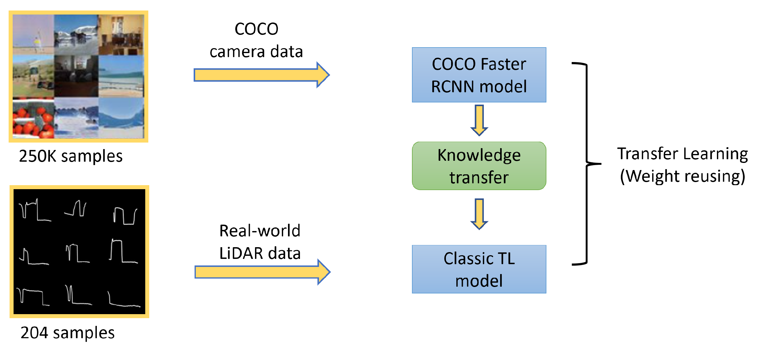
- Comparison of transfer learning with and without synthetic data:
- -
- From camera-based real-world data to our LiDAR capture data.
- -
- From camera-based real-world data via a large synthetic data set, which synthesises our real-world data set accurately to our LiDAR capture data.
- This comparison demonstrates in our application that Synthetically Augmented Transfer Learning contributes to an increase in the performance of the classification model.
3. Methodology
4. Synthetic Data
4.1. Data Generation
4.2. Implementation and Fundamentals
4.3. Data Simulations
4.3.1. Vehicle Rotations
4.3.2. Creating Varied Scenes
4.3.3. Parameters and Assumptions
4.4. Synthetic Training and Results
5. Real-World Data
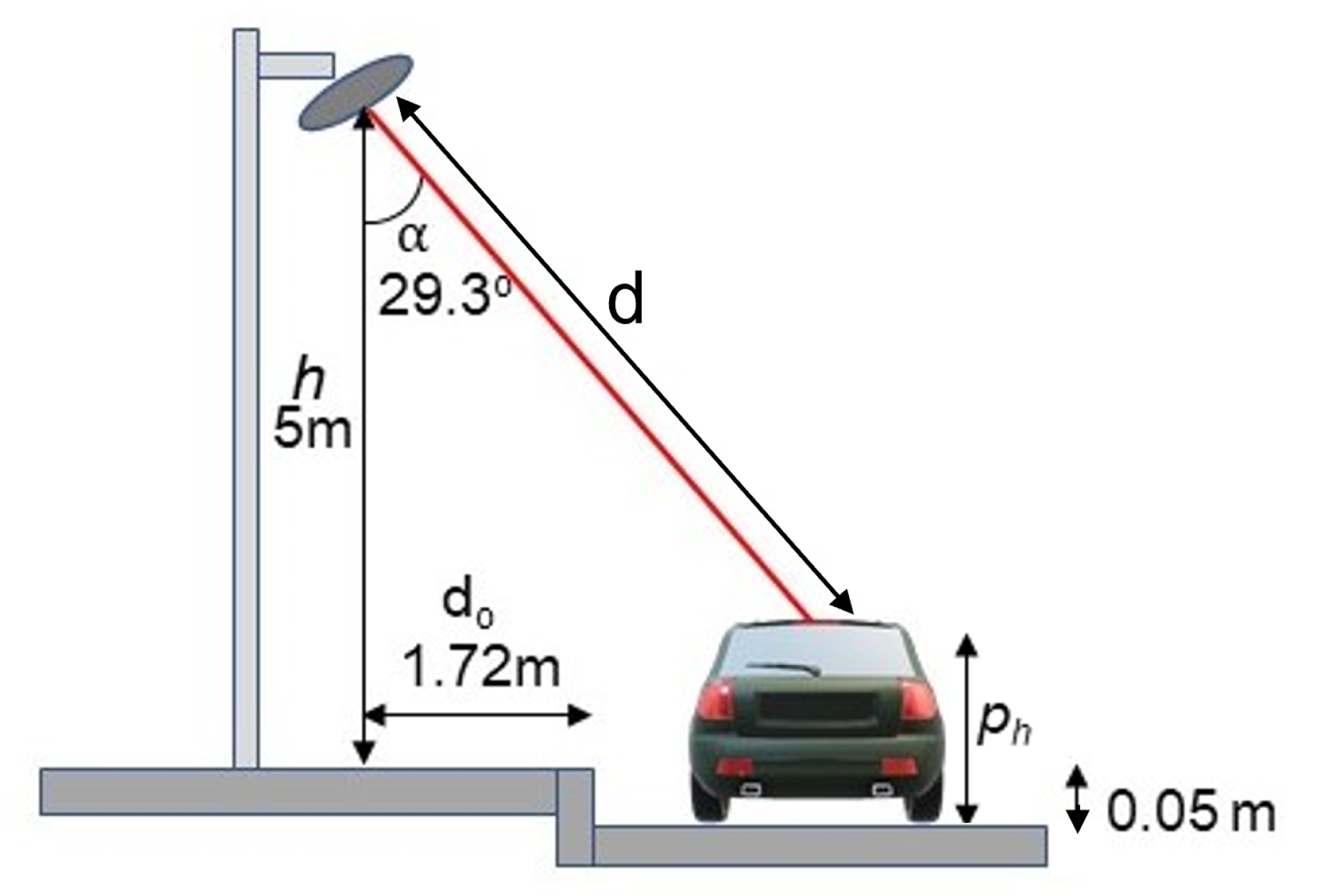
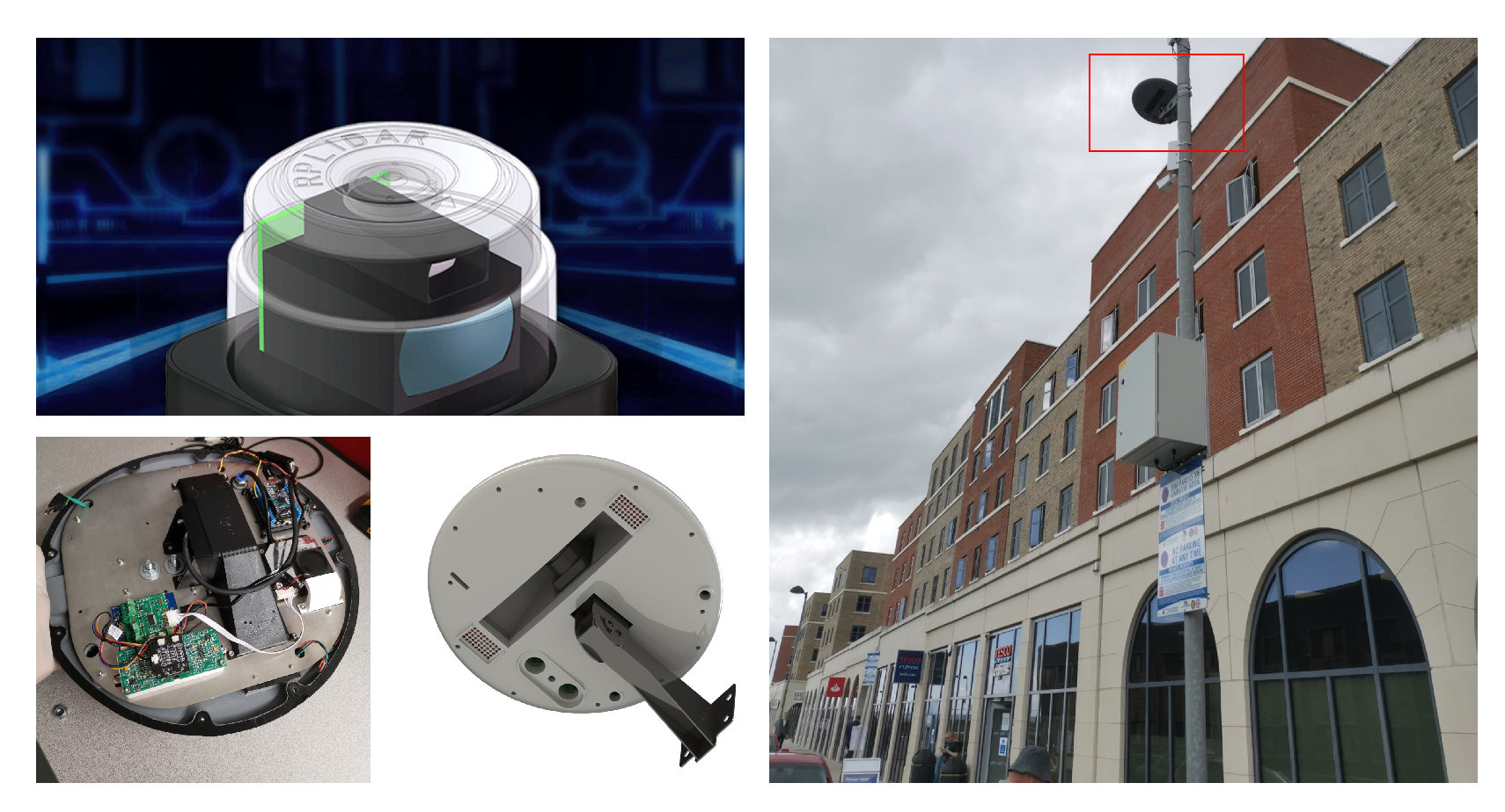
5.1. Hardware Installation of LiDAR Sensor
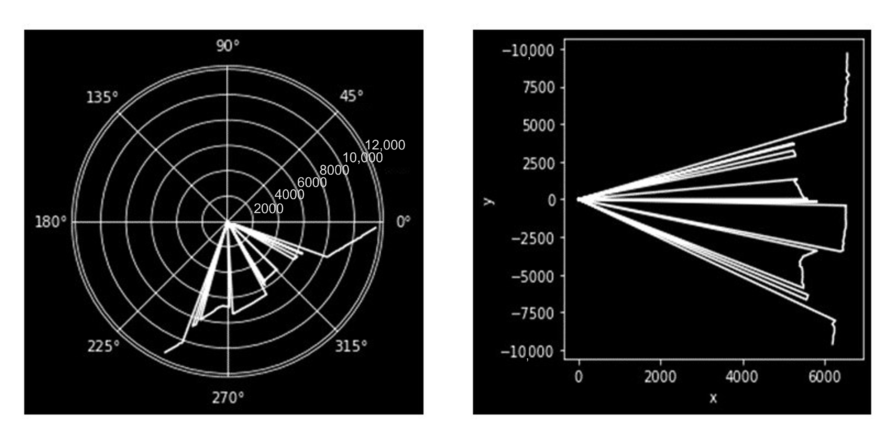
5.2. LiDAR Data Retrieval and Processing
- Eliminate LiDAR points appearing too close to the detector. The LiDAR can return very small or zero distance values in place of true values in some conditions.
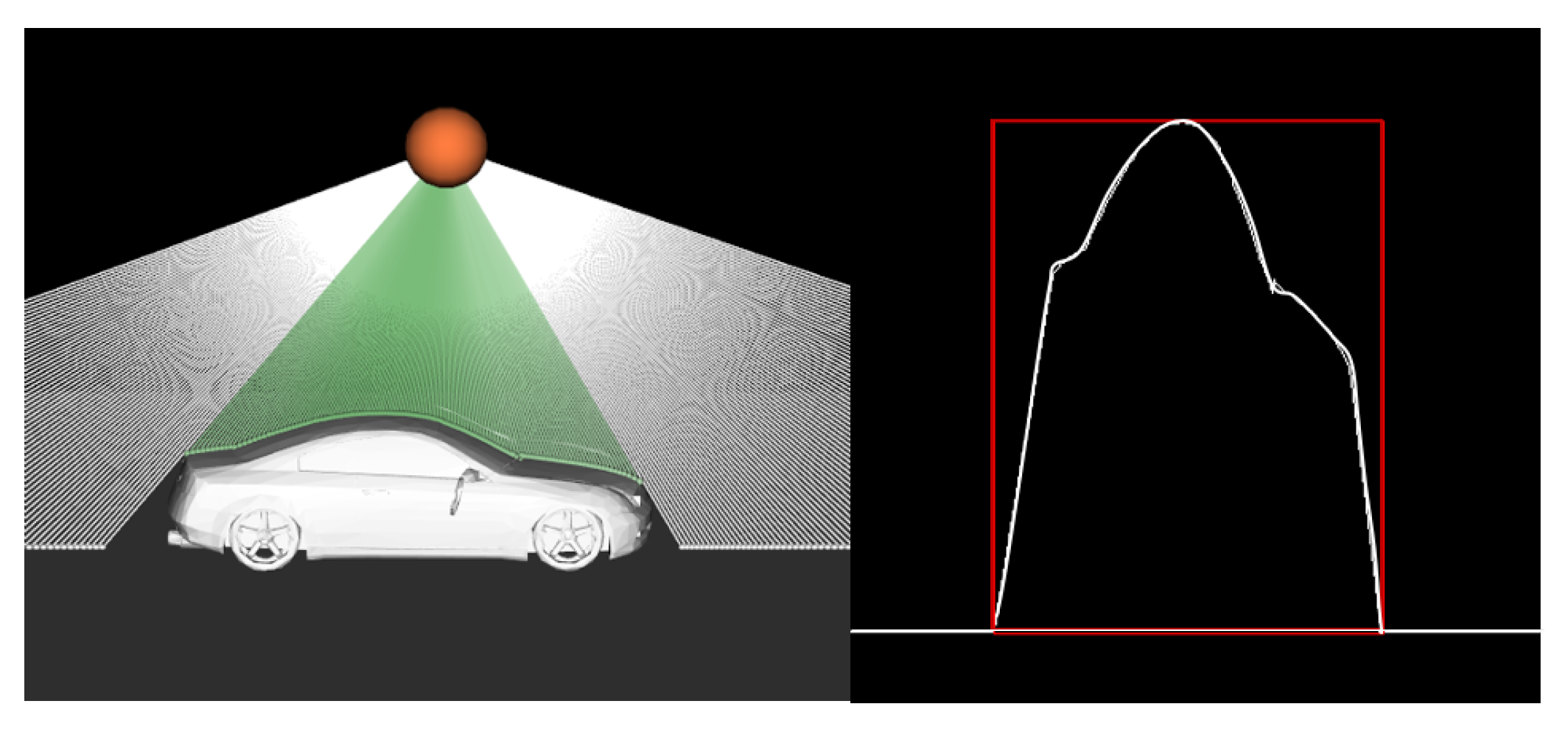
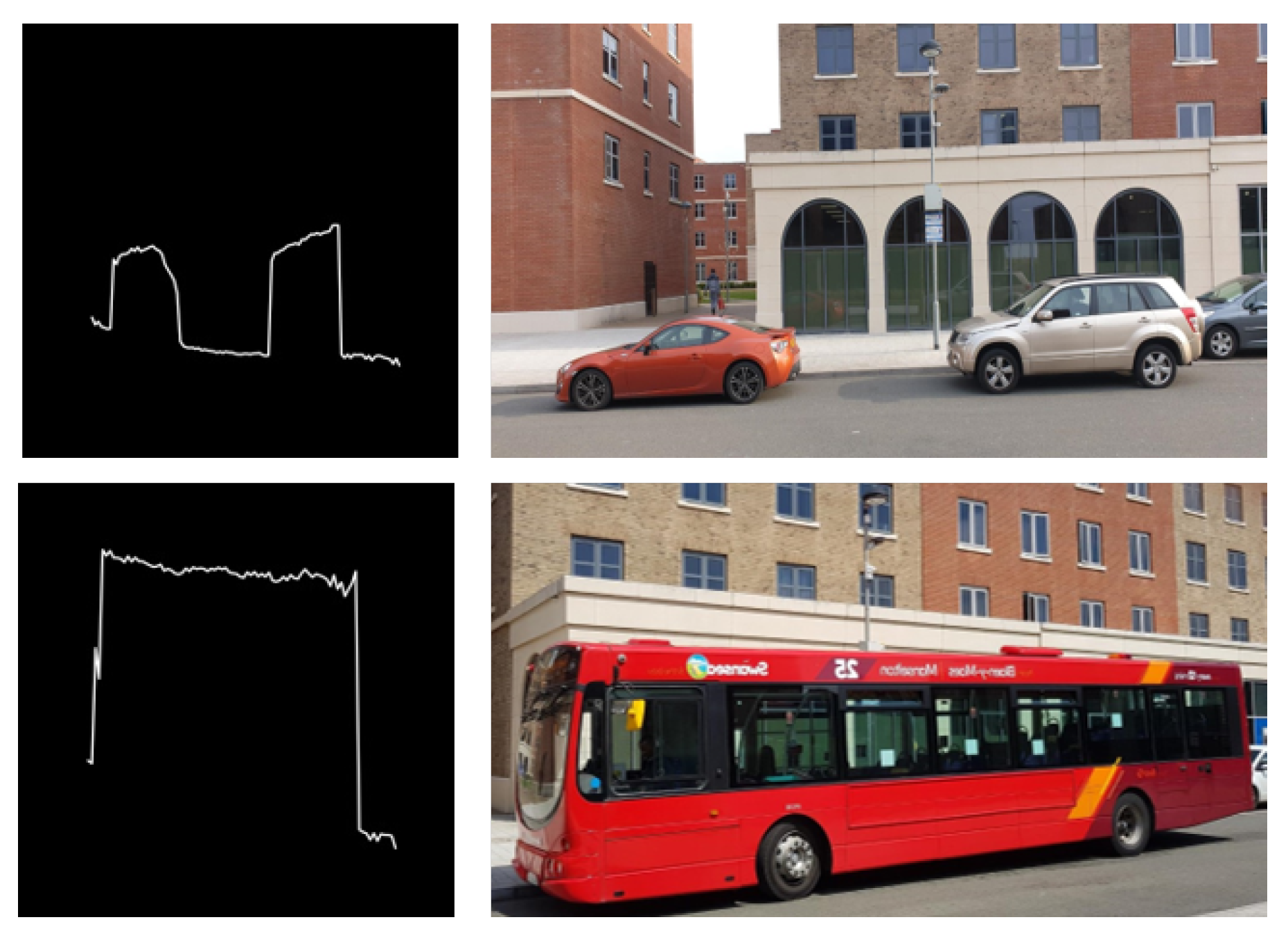
- Restrict the data between 3000 and 7000 mm to obtain only vehicle profiles in the Cartesian plot in Figure 12.
- Remove the image when there are no vehicles parked on the road by limiting x between 6000 and 7000 in the Cartesian plot in Figure 12.
- Remove any LiDAR images that occasionally produce an insufficient profile, that is, when the vehicle profile is not adequately caught; for instance when LiDAR takes a profile of a fast-moving vehicle, it simply captures a vertical line that represents nothing.
- Re-scale the image by restricting the x and y-axis to match the profile of synthetic data.
5.3. Creating Ground Truth Labelled Data
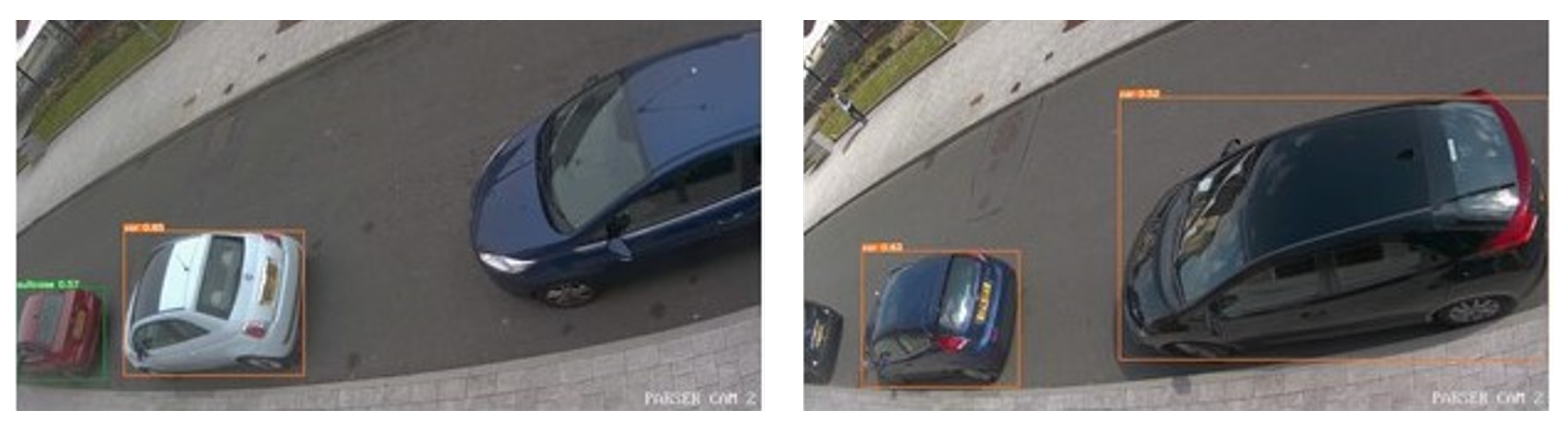
6. Comparative TL Model Results Tested on Real-World LiDAR Data
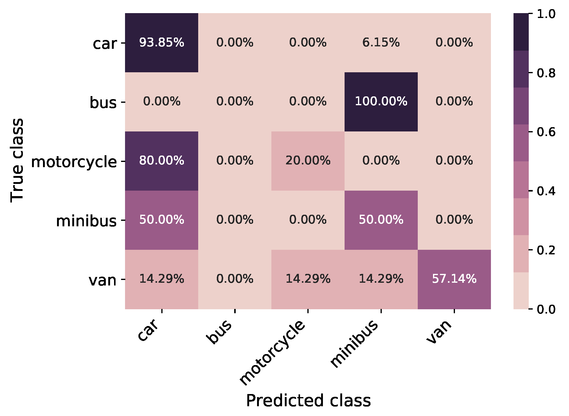
6.1. Classic TL Model
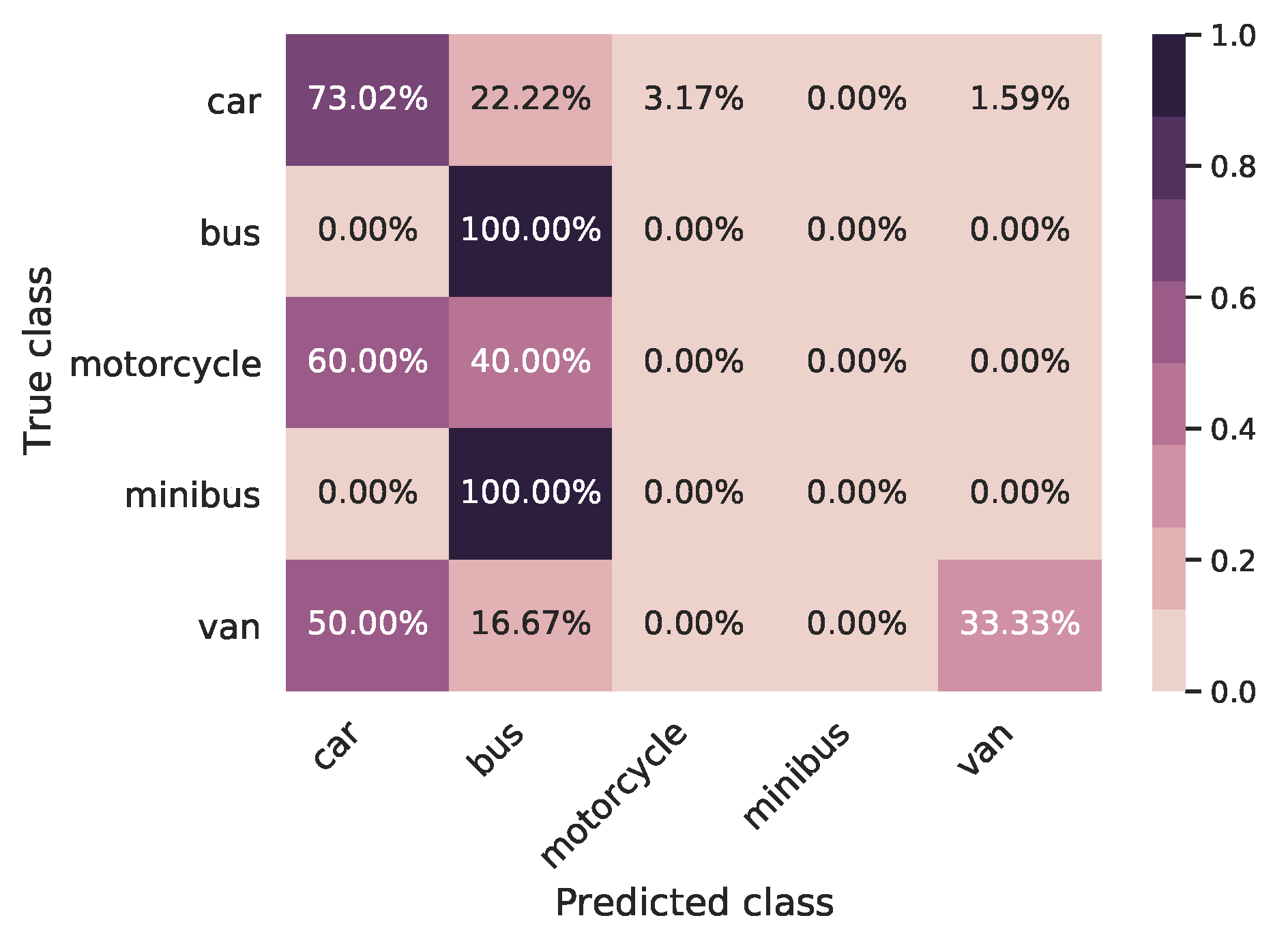
6.2. Synthetic TL Model
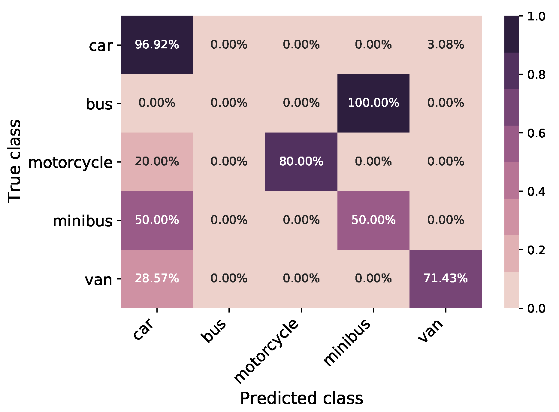
6.3. Synthetically Augmented TL Model
- Null hypothesis : There is no difference between the synthetically augmented TL model and the classic TL model.
- Alternative hypothesis : The synthetically augmented TL model exhibits higher performance than the classic TL model.
7. Conclusions
Author Contributions
Funding
Institutional Review Board Statement
Informed Consent Statement
Data Availability Statement
Acknowledgments
Conflicts of Interest
References
- British Parking Association. Available online: https://www.britishparking.co.uk/Library-old/Blueprint-for-Parking-2017-2021/136174 (accessed on 21 January 2023).
- Thornton, D.A.; Redmill, K.; Coifman, B. Automated parking surveys from a LIDAR equipped vehicle. Transp. Res. Part C Emerg. Technol. 2014, 39, 23–35. [Google Scholar] [CrossRef]
- De Cerreño, A.L. Dynamics of on-street parking in large central cities. Transp. Res. Rec. 2004, 1898, 130–137. [Google Scholar] [CrossRef]
- Zhao, P.; Guan, H.; Wang, P. Data-driven robust optimal allocation of shared parking spaces strategy considering uncertainty of public users’ and owners’ arrival and departure: An agent-based approach. IEEE Access 2020, 8, 24182–24195. [Google Scholar] [CrossRef]
- Chai, H.; Ma, R.; Zhang, H.M. Search for parking: A dynamic parking and route guidance system for efficient parking and traffic management. J. Intell. Transp. Syst. 2019, 23, 541–556. [Google Scholar] [CrossRef]
- Chen, S.; Chen, Y.; Zhang, S.; Zheng, N. A novel integrated simulation and testing platform for self-driving cars with hardware in the loop. IEEE Trans. Intell. Veh. 2019, 4, 425–436. [Google Scholar] [CrossRef]
- Yuan, Y.; Van Lint, H.; Van Wageningen-Kessels, F.; Hoogendoorn, S. Network-wide traffic state estimation using loop detector and floating car data. J. Intell. Transp. Syst. 2014, 18, 41–50. [Google Scholar] [CrossRef]
- Barceló, J.; Kuwahara, M.; Miska, M. Traffic Data Collection and Its Standardization; Springer: Berlin/Heidelberg, Germany, 2010. [Google Scholar]
- Yang, Z.; Pun-Cheng, L.S. Vehicle detection in intelligent transportation systems and its applications under varying environments: A review. Image Vis. Comput. 2018, 69, 143–154. [Google Scholar] [CrossRef]
- Díaz, J.J.V.; González, A.B.R.; Wilby, M.R. Bluetooth traffic monitoring systems for travel time estimation on freeways. IEEE Trans. Intell. Transp. Syst. 2015, 17, 123–132. [Google Scholar] [CrossRef]
- Lv, B.; Xu, H.; Wu, J.; Tian, Y.; Zhang, Y.; Zheng, Y.; Yuan, C.; Tian, S. LiDAR-enhanced connected infrastructures sensing and broadcasting high-resolution traffic information serving smart cities. IEEE Access 2019, 7, 79895–79907. [Google Scholar] [CrossRef]
- Du, X.; Ang, M.H.; Rus, D. Car detection for autonomous vehicle: LIDAR and vision fusion approach through deep learning framework. In Proceedings of the 2017 IEEE/RSJ International Conference on Intelligent Robots and Systems (IROS), Vancouver, BC, Canada, 24–28 September 2017; IEEE: Piscataway, NJ, USA, 2017; pp. 749–754. [Google Scholar]
- Chavez-Garcia, R.O.; Aycard, O. Multiple sensor fusion and classification for moving object detection and tracking. IEEE Trans. Intell. Transp. Syst. 2015, 17, 525–534. [Google Scholar] [CrossRef]
- Liu, W.; Xia, X.; Xiong, L.; Lu, Y.; Gao, L.; Yu, Z. Automated vehicle sideslip angle estimation considering signal measurement characteristic. IEEE Sens. J. 2021, 21, 21675–21687. [Google Scholar] [CrossRef]
- Pan, S.J.; Kwok, J.T.; Yang, Q. Transfer learning via dimensionality reduction. In Proceedings of the AAAI, Chicago, IL, USA, 13–17 July 2008; Volume 8, pp. 677–682. [Google Scholar]
- Douarre, C.; Schielein, R.; Frindel, C.; Gerth, S.; Rousseau, D. Transfer learning from synthetic data applied to soil–root segmentation in X-ray tomography images. J. Imaging 2018, 4, 65. [Google Scholar] [CrossRef]
- Jung, S.; Park, J.; Lee, S. Polyphonic sound event detection using convolutional bidirectional lstm and synthetic data-based transfer learning. In Proceedings of the 2019 IEEE International Conference on Acoustics, Speech and Signal Processing (ICASSP 2019), Brighton, UK, 12–17 May 2019; IEEE: Piscataway, NJ, USA, 2019; pp. 885–889. [Google Scholar]
- Liu, W.; Quijano, K.; Crawford, M.M. YOLOv5-Tassel: Detecting tassels in RGB UAV imagery with improved YOLOv5 based on transfer learning. IEEE J. Sel. Top. Appl. Earth Obs. Remote Sens. 2022, 15, 8085–8094. [Google Scholar] [CrossRef]
- Xiao, A.; Huang, J.; Guan, D.; Zhan, F.; Lu, S. Transfer learning from synthetic to real LiDAR point cloud for semantic segmentation. arXiv 2021, arXiv:2107.05399. [Google Scholar] [CrossRef]
- Weiss, K.; Khoshgoftaar, T.M.; Wang, D. A survey of transfer learning. J. Big Data 2016, 3, 1–40. [Google Scholar] [CrossRef]
- Pan, S.J.; Yang, Q. A survey on transfer learning. IEEE Trans. Knowl. Data Eng. 2010, 22, 1345–1359. [Google Scholar] [CrossRef]
- Hu, H.N.; Cai, Q.Z.; Wang, D.; Lin, J.; Sun, M.; Krahenbuhl, P.; Darrell, T.; Yu, F. Joint monocular 3D vehicle detection and tracking. In Proceedings of the IEEE/CVF International Conference on Computer Vision, Seoul, Republic of Korea, 27 October–2 November 2019; pp. 5390–5399. [Google Scholar]
- Broome, M.; Gadd, M.; De Martini, D.; Newman, P. On the road: Route proposal from radar self-supervised by fuzzy LiDAR traversability. AI 2020, 1, 558–585. [Google Scholar] [CrossRef]
- Lee, H.; Coifman, B. Side-Fire Lidar-Based Vehicle Classification. Transp. Res. Rec. 2012, 2308, 173–183. [Google Scholar] [CrossRef]
- Sandhawalia, H.; Rodriguez-Serrano, J.A.; Poirier, H.; Csurka, G. Vehicle type classification from laser scanner profiles: A benchmark of feature descriptors. In Proceedings of the 16th International IEEE Conference on Intelligent Transportation Systems (ITSC 2013), The Hague, The Netherlands, 6–9 October 2013; pp. 517–522. [Google Scholar]
- Sun, Y.; Xu, H.; Wu, J.; Zheng, J.; Dietrich, K.M. 3-D Data Processing to Extract Vehicle Trajectories from Roadside LiDAR Data. Transp. Res. Rec. 2018, 2672, 14–22. [Google Scholar] [CrossRef]
- Nashashibi, F.; Bargeton, A. Laser-based vehicles tracking and classification using occlusion reasoning and confidence estimation. In Proceedings of the 2008 IEEE Intelligent Vehicles Symposium, Eindhoven, The Netherlands, 4–6 June 2008; IEEE: Piscataway, NJ, USA, 2008; pp. 847–852. [Google Scholar]
- Wu, J.; Xu, H.; Zheng, Y.; Zhang, Y.; Lv, B.; Tian, Z. Automatic Vehicle Classification using Roadside LiDAR Data. Transp. Res. Rec. 2019, 2673, 153–164. [Google Scholar] [CrossRef]
- Habermann, D.; Hata, A.; Wolf, D.; Osório, F.S. Artificial neural nets object recognition for 3D point clouds. In Proceedings of the 2013 Brazilian Conference on Intelligent Systems, Fortaleza, Brazil, 19–24 October 2013; IEEE: Piscataway, NJ, USA, 2013; pp. 101–106. [Google Scholar]
- Pang, G.; Neumann, U. 3D point cloud object detection with multi-view convolutional neural network. In Proceedings of the 2016 23rd International Conference on Pattern Recognition (ICPR), Cancun, Mexico, 4–8 December 2016; IEEE: Piscataway, NJ, USA, 2016; pp. 585–590. [Google Scholar]
- Huang, L.; Yang, Y.; Deng, Y.; Yu, Y. DenseBox: Unifying Landmark Localization with End to End Object Detection. arXiv 2015, arXiv:1509.04874. [Google Scholar]
- Sermanet, P.; Eigen, D.; Zhang, X.; Mathieu, M.; Fergus, R.; LeCun, Y. OverFeat: Integrated Recognition, Localization and Detection using Convolutional Networks. arXiv 2013, arXiv:1312.6229. [Google Scholar]
- Li, B.; Zhang, T.; Xia, T. Vehicle Detection from 3D Lidar Using Fully Convolutional Network. arXiv 2016, arXiv:1608.07916. [Google Scholar]
- Chen, X.; Ma, H.; Wan, J.; Li, B.; Xia, T. Multi-view 3D object detection network for autonomous driving. In Proceedings of the IEEE Conference on Computer Vision and Pattern Recognition, Honolulu, HI, USA, 21–26 July 2017; pp. 1907–1915. [Google Scholar]
- The KITTI Vision Benchmark Suite. 2015. Available online: http://www.cvlibs.net/datasets/kitti (accessed on 21 November 2022).
- Redmon, J.; Divvala, S.; Girshick, R.; Farhadi, A. You Only Look Once: Unified, Real-Time Object Detection. arXiv 2015, arXiv:1506.02640. [Google Scholar]
- Girshick, R. Fast R-CNN. arXiv 2015, arXiv:1504.08083. [Google Scholar]
- Wang, H.; Yu, Y.; Cai, Y.; Chen, X.; Chen, L.; Liu, Q. A comparative study of state-of-the-art deep learning algorithms for vehicle detection. IEEE Intell. Transp. Syst. Mag. 2019, 11, 82–95. [Google Scholar] [CrossRef]
- Tourani, A.; Soroori, S.; Shahbahrami, A.; Khazaee, S.; Akoushideh, A. A robust vehicle detection approach based on faster R-CNN algorithm. In Proceedings of the 2019 4th International Conference on Pattern Recognition and Image Analysis (IPRIA), Tehran, Iran, 6–7 March 2019; IEEE: Piscataway, NJ, USA, 2019; pp. 119–123. [Google Scholar]
- Xu, Q.; Zhang, X.; Cheng, R.; Song, Y.; Wang, N. Occlusion problem-oriented adversarial faster-RCNN scheme. IEEE Access 2019, 7, 170362–170373. [Google Scholar] [CrossRef]
- Wang, Y.; Deng, W.; Liu, Z.; Wang, J. Deep learning-based vehicle detection with synthetic image data. IET Intell. Transp. Syst. 2019, 13, 1097–1105. [Google Scholar] [CrossRef]
- Tremblay, J.; Prakash, A.; Acuna, D.; Brophy, M.; Jampani, V.; Anil, C.; To, T.; Cameracci, E.; Boochoon, S.; Birchfield, S. Training deep networks with synthetic data: Bridging the reality gap by domain randomization. In Proceedings of the IEEE Conference on Computer Vision and Pattern Recognition Workshops, Salt Lake City, UT, USA, 18–22 June 2018; pp. 969–977. [Google Scholar]
- de Melo, C.M.; Torralba, A.; Guibas, L.; DiCarlo, J.; Chellappa, R.; Hodgins, J. Next-generation deep learning based on simulators and synthetic data. Trends Cogn. Sci. 2021, 26, 174–187. [Google Scholar] [CrossRef]
- Lakshmanan, K.; Gil, A.J.; Auricchio, F.; Tessicini, F. A fault diagnosis methodology for an external gear pump with the use of Machine Learning classification algorithms: Support Vector Machine and Multilayer Perceptron. Loughborough University Research Repository. 2020. Available online: https://repository.lboro.ac.uk/articles/conference_contribution/A_fault_diagnosis_methodology_for_an_external_gear_pump_with_the_use_of_Machine_Learning_classification_algorithms_Support_Vector_Machine_and_Multilayer_Perceptron/12097668/1 (accessed on 21 January 2023).
- Torrey, L.; Shavlik, J. Transfer learning. In Handbook of Research on Machine Learning Applications and Trends: Algorithms, Methods, and Techniques; IGI Global: Hershey, PA, USA, 2010; pp. 242–264. [Google Scholar]
- Pan, W.; Xiang, E.; Liu, N.; Yang, Q. Transfer learning in collaborative filtering for sparsity reduction. In Proceedings of the AAAI Conference on Artificial Intelligence, Atlanta, GA, USA, 11–15 July 2010; Volume 24. [Google Scholar]
- Tan, C.; Sun, F.; Kong, T.; Zhang, W.; Yang, C.; Liu, C. A survey on deep transfer learning. In Proceedings of the International Conference on Artificial Neural Networks, Rhodes, Greece, 4–7 October 2018; Springer International Publishing: Cham, Switzerland, 2018; pp. 270–279. [Google Scholar]
- Cunha, A.; Pochet, A.; Lopes, H.; Gattass, M. Seismic fault detection in real data using transfer learning from a convolutional neural network pre-trained with synthetic seismic data. Comput. Geosci. 2020, 135, 104344. [Google Scholar] [CrossRef]
- Gao, Y.; Mosalam, K.M. Deep transfer learning for image-based structural damage recognition. Comput.-Aided Civ. Infrastruct. Eng. 2018, 33, 748–768. [Google Scholar] [CrossRef]
- Goodfellow, I.; Bengio, Y.; Courville, A. Deep Learning; MIT Press: Cambridge, MA, USA, 2016. [Google Scholar]
- Huang, J.; Rathod, V.; Sun, C.; Zhu, M.; Korattikara, A.; Fathi, A.; Fischer, I.; Wojna, Z.; Song, Y.; Guadarrama, S.; et al. Speed/accuracy trade-offs for modern convolutional object detectors. In Proceedings of the IEEE Conference on Computer Vision and Pattern Recognition, Honolulu, HI, USA, 21–26 July 2017; pp. 7310–7311. [Google Scholar]
- Chang, A.X.; Funkhouser, T.; Guibas, L.; Hanrahan, P.; Huang, Q.; Li, Z.; Savarese, S.; Savva, M.; Song, S.; Su, H.; et al. ShapeNet: An Information-Rich 3D Model Repository. arXiv 2015, arXiv:1512.03012. [Google Scholar]
- Visualisation Toolkit. Available online: https://vtk.org/?msclkid=c10ed6e5d13111ecbd9df41841d1b5f3 (accessed on 21 January 2023).
- Yu, H.; Chen, C.; Du, X.; Li, Y.; Rashwan, A.; Hou, L.; Jin, P.; Yang, F.; Liu, F.; Kim, J.; et al. TensorFlow Model Garden. 2020. Available online: https://github.com/tensorflow/models (accessed on 21 January 2023).
- RPLIDAR S1 Portable TOF Laser Range Scanner. Available online: https://www.slamtec.com/en/Lidar/S1 (accessed on 21 January 2023).
- Redmon, J.; Farhadi, A. YOLO9000: Better, Faster, Stronger. In Proceedings of the 2017 IEEE Conference on Computer Vision and Pattern Recognition (CVPR), Honolulu, HI, USA, 21–26 July 2017; pp. 6517–6525. [Google Scholar]
- Object Detection Yolo5 Implementation. 2022. Available online: https://github.com/maheshlaksh05/Object-Detection-Yolo5-Implementation (accessed on 21 January 2023).
- Bochkovskiy, A.; Wang, C.Y.; Liao, H.Y.M. Yolov4: Optimal speed and accuracy of object detection. arXiv 2020, arXiv:2004.10934. [Google Scholar]
- Deng, J.; Dong, W.; Socher, R.; Li, L.J.; Li, K.; Li, F.-F. Imagenet: A large-scale hierarchical image database. In Proceedings of the 2009 IEEE Conference on Computer Vision and Pattern Recognition, Miami, FL, USA, 20–25 June 2009; IEEE: Piscataway, NJ, USA, 2009; pp. 248–255. [Google Scholar]


| Parameter | Description | Type | Value | |
|---|---|---|---|---|
| LiDAR Height | h | The vertical distance between the LiDAR and the pavement | Fixed | 5 m |
| LiDAR Road Offset | The horizontal distance between the LiDAR and the curb of the road | Fixed | 1.72 m | |
| LiDAR Angle | The angle at which the LiDAR is positioned to monitor the road | Fixed | ||
| LiDAR Increment Angle | The angle which the LiDAR sensor moves between scans | Fixed | ||
| Arc of Interest | Angle limits dictating an arc of readings | Fixed | ||
| Sweep Frequency | The frequency with which the LiDAR repeats | Fixed | Hz | |
| Sweep Time | The time it takes the LiDAR to perform a full sweep of all angles | Fixed | 0 s | |
| Scan Range | The length from the device the LiDAR will return a reading | Fixed | 12 M | |
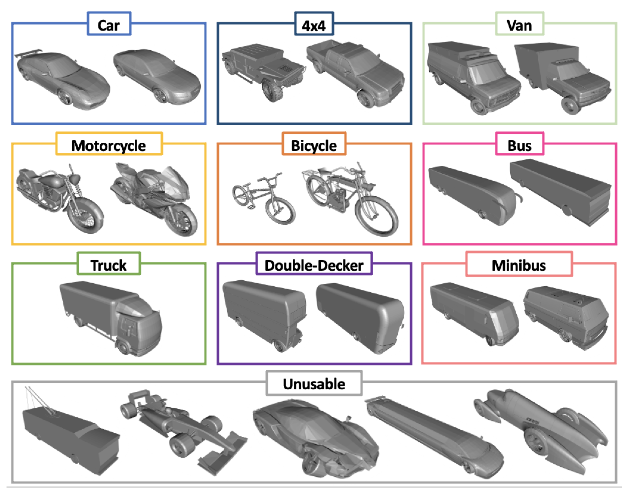
| Vehicle Type | Vehicle from ShapeNet data set, | Variable | ||
| Vehicle Scale | The 3D scale of the vehicle with respect to the scene and other vehicles in the data set | Fixed | ||
| Vehicle Driving Direction | If the vehicle is driving forward, F, or backwards, B | Variable | ||
| Vehicle Angle | The angle of the vehicle with respect to the road curb | Variable | ||
| Samples per Revolution | Individual LiDAR readings per full revolution | Derived | 720 | |
| Samples per Second | Total LiDAR readings per second | Derived | 3960 | |
| Samples in Sweep per Second | Total LiDAR readings per second in Arc of Interest | Derived | 1320 | |
| Multiple parked vehicles | Total number of vehicle parked on the scene | Fixed | 5 | |
| Assumption | Description | |||
| LiDAR Increment Angle | is constant, meaning each time the sensor rotates, it is by a constant value | |||
| Samples per Revolution | is a whole number, this means that for each revolution of the LiDAR there is no drift | |||
| resulting in a single full revolution each sweep based on the above assumptions | ||||
| LiDAR is directly above the moving vehicle, and the sweep is perpendicular to the road | ||||
| The LiDAR sweep is instantaneous for computational efficiency |
| Class | Bounding Box | Timestamp | Prediction Score | Daytime Flag |
|---|---|---|---|---|
| Car | [0.9189, 0.2878, 0.1621, 0.3576] | 2021-08-13 05:44:24 | 0.48485 | Night |
| Truck | [0.0471, 0.7732, 0.0884, 0.3076] | 2021-08-13 10:55:05 | 0.46900 | Day |
| Car | [0.0470, 0.7746, 0.0902, 0.3006] | 2021-08-13 10:55:05 | 0.49065 | Day |
| Car | [0.8817, 0.8777, 0.2341, 0.2444] | 2021-08-13 18:06:41 | 0.74662 | Day |
| Car | [0.1920, 0.2434, 0.1447, 0.4270] | 2021-08-13 18:06:41 | 0.84887 | Day |
| Car | [0.8153, 0.2673, 0.1962, 0.3569] | 2021-08-13 18:06:41 | 0.90770 | Day |
| Car | [0.8817, 0.8718, 0.2341, 0.2548] | 2021-08-13 18:07:13 | 0.59120 | Day |
| Model | Accuracy | Error Reduction | F1 Score | Error Reduction | IOU Mean | IOU Variance | Computation Time |
|---|---|---|---|---|---|---|---|
| Classic transfer learning (CTL) | 83.75% | N/A | 0.837 | N/A | 0.418 | 0.272 | 688.006 s |
| Synthetic TL model | 61.25% | −58.73% | 0.605 | −58.06% | 0.252 | 0.211 | 17250 s |
| Synthetic augmented TL (weight reusing) | 91.25% | 46.15% | 0.906 | 40.81% | 0.520 | 0.273 | 693.86 s |
| Synthetic augmented TL (feature extraction) | 86.25% | 36.3% | 0.872 | 26.5% | 0.494 | 0.263 | 688.01 s |
Disclaimer/Publisher’s Note: The statements, opinions and data contained in all publications are solely those of the individual author(s) and contributor(s) and not of MDPI and/or the editor(s). MDPI and/or the editor(s) disclaim responsibility for any injury to people or property resulting from any ideas, methods, instructions or products referred to in the content. |
© 2023 by the authors. Licensee MDPI, Basel, Switzerland. This article is an open access article distributed under the terms and conditions of the Creative Commons Attribution (CC BY) license (https://creativecommons.org/licenses/by/4.0/).
Share and Cite
Lakshmanan, K.; Roach, M.; Giannetti, C.; Bhoite, S.; George, D.; Mortensen, T.; Manduhu, M.; Heravi, B.; Kariyawasam, S.; Xie, X. A Robust Vehicle Detection Model for LiDAR Sensor Using Simulation Data and Transfer Learning Methods. AI 2023, 4, 461-481. https://doi.org/10.3390/ai4020025
Lakshmanan K, Roach M, Giannetti C, Bhoite S, George D, Mortensen T, Manduhu M, Heravi B, Kariyawasam S, Xie X. A Robust Vehicle Detection Model for LiDAR Sensor Using Simulation Data and Transfer Learning Methods. AI. 2023; 4(2):461-481. https://doi.org/10.3390/ai4020025
Chicago/Turabian StyleLakshmanan, Kayal, Matt Roach, Cinzia Giannetti, Shubham Bhoite, David George, Tim Mortensen, Manduhu Manduhu, Behzad Heravi, Sharadha Kariyawasam, and Xianghua Xie. 2023. "A Robust Vehicle Detection Model for LiDAR Sensor Using Simulation Data and Transfer Learning Methods" AI 4, no. 2: 461-481. https://doi.org/10.3390/ai4020025