
Can Interpretable Reinforcement Learning Manage Prosperity Your Way?


1
Chief Technology Office, Sparebank 1 SR-Bank, 4007 Stavanger, Norway
2
Center for AI Research, University of Agder, 4879 Grimstad, Norway
*
Author to whom correspondence should be addressed.
†
Current address: Jon Lilletunsvei 9, 4879 Grimstad, Norway.
AI 2022, 3(2), 526-537; https://doi.org/10.3390/ai3020030
Submission received: 6 May 2022
/
Revised: 30 May 2022
/
Accepted: 10 June 2022
/
Published: 13 June 2022
(This article belongs to the Special Issue Feature Papers for AI)
Abstract
:Personalisation of products and services is fast becoming the driver of success in banking and commerce. Machine learning holds the promise of gaining a deeper understanding of and tailoring to customers’ needs and preferences. Whereas traditional solutions to financial decision problems frequently rely on model assumptions, reinforcement learning is able to exploit large amounts of data to improve customer modelling and decision-making in complex financial environments with fewer assumptions. Model explainability and interpretability present challenges from a regulatory perspective which demands transparency for acceptance; they also offer the opportunity for improved insight into and understanding of customers. Post-hoc approaches are typically used for explaining pretrained reinforcement learning models. Based on our previous modeling of customer spending behaviour, we adapt our recent reinforcement learning algorithm that intrinsically characterizes desirable behaviours and we transition to the problem of prosperity management. We train inherently interpretable reinforcement learning agents to give investment advice that is aligned with prototype financial personality traits which are combined to make a final recommendation. We observe that the trained agents’ advice adheres to their intended characteristics, they learn the value of compound growth, and, without any explicit reference, the notion of risk as well as improved policy convergence.
1. Introduction
Personalization is critical in modern retail services, and banking is no exception. Financial service providers are employing ever-advancing methods to improve the level of personalisation of their services [1,2]. Artificial intelligence (AI) is a promising tool in this pursuit in areas such as anti-money laundering, trading and investment, and customer relationship management [3]. Examples of personalised services are recommender systems for product sales [4], risk evaluation for credit scoring [5], and segmentation for customer-centric marketing [6]. More commonly, AI has been applied to stock trading via ensemble learning [7], currency recognition using deep learning [8], stock index performance through time-series modelling with feature engineering [9], and investment portfolio management using reinforcement learning (RL) [10,11]. These applications generally lack the personalisation needed to enhance customer relations and support service delivery for growing customer bases. We address the issue of personalization by using an interpretable RL algorithm to manage a portfolio of various asset classes according to individual spending behaviour. Whereas the current literature is only concerned with portfolio optimization, our objective is a more holistic prosperity management service, which includes a more diverse portfolio of asset classes. Such a service might improve customer interaction through personalization, enhance trust through interpretability, and contribute to customer acquisition and retention.
The lack of explainability and interpretability has thus far hindered the wider adoption of machine learning, mainly due to model opacity; model understanding is essential in financial services [12,13,14]. We distinguish between explainability and interpretability: explainability refers to a symbolic representation of the knowledge a model has learned, while interpretability is necessary for reasoning about a model’s predictions. We have previously investigated the interpretability of systems of multiple RL agents [15]: a regularisation term in the objective function instilled a desired agent behaviour during training. For our current purpose of prosperity management, we create prototypical RL agents which have intrinsic affinities for certain asset classes. They have characteristic asset allocation strategies which are easy to interpret. The asset allocation preference of a real customer is an amalgam of the strategies which can be realized by a composition of the prototypical RL agents. Unlike work reported in [16] that investigate Boolean composition of RL agents, our challenge is to determine a RL agent composition which is a reflection of real customer preferences. In this paper, we investigate the efficacy of linear compositions of prototypical RL agents which represent real customers; the coefficients in these linear compositions are the fuzzy memberships of customers’ prototypical personality traits. We rate asset classes, such as stocks and savings accounts, in terms of their inherent properties, such as expected long term risk and reward, and liquidity. For each asset class property, we define an association with the prototypical personality traits [17]. We derive the agents’ affinities for certain asset classes as the inner product of these associations and the asset class ratings. Their intrinsic interpretability may fulfill the promise of a digital private assistant for personal wealth management.
We introduce the relevant theoretical background in the next section, after which we discuss our methodology and list a set of key assumptions, present and discuss and our results, and conclude with a discussion and suggestions for future work.
2. Related Work
Recent evidence has revealed a causal relationship between spending patterns and individual happiness [18]: we are happiest when our spending matches our personality. For instance, extraverted individuals typically prefer spending at a bar rather than at a bookshop, while the opposite may apply to introverts. Our premise is that spending personality traits can be carried over to prosperity management: we are happiest when our investment matches our personality. For instance, conscientious investors may prefer the predictability of property over the volatility of stocks. This is consistent with the high affinity of conscientious spenders towards residential mortgages [18]. It is compelling to expand the notion of personality traits from spending to wealth creation, i.e., to base personal investment advice on historical spending behaviour [19,20].
In RL, agents learn by trial and error to maximize the expected cumulative reward given by the environment in which they act [21]. Their actions result in changing the internal state of the environment, which is known to the agents through observations. RL agents are adept at maximising future rewards despite potential sparse or immediate negative rewards [21]. The environment is modelled as a Markov decision process (MDP), which is a discrete-time stochastic process in which the core underlying assumption is that the state of the environment depends solely on its previous state and the action taken by the agent [22]. It is described by the set where S is a set of states, A a set of actions, the probability that action a in state s will lead to state , and is the reward given for action a in state s. Deep deterministic policy gradient (DDPG [23]) is a RL algorithm that represents an agent through two neural networks: an actor and a critic. The actor takes the state observation as input and predicts the best action, while the critic takes the state observation and predicted action as input and predicts the reward from the environment. While the critic learns the dynamics of the environment, the agent learns to maximize the predicted reward. For numerical stability and to improve convergence, DDPG initializes two identical target networks for the actor and critic, respectively. The parameters of these target networks are slowly updated, as specified by the target update hyperparameter.
RL has been extensively applied to stock portfolio management [24,25,26,27,28,29], but not yet to holistic prosperity management; the lack of model transparency may be a contributing factor. Interpretation of RL agents typically follows model training [30,31,32]; our ambition is to impose a desired characteristic behaviour during training, thus making it an intrinsic property of the agent. Based on a prior that defines a desired behaviour, we extend the DDPG objective function with a regularisation term [15]. Formally, for each agent i, this objective function is given by:
where is a set of parameters governing the policy, is the replay buffer, is the reward for action with the partial sate observation , is a scaling parameter, is the number of actions, and is the prior that defines the desired behaviour of the agent. Note that the prior is independent of the state, which simplifies it and thus makes it interpretable; this is a departure from traditional policy regularisation methods such as KL-regularisation and entropy regularisation which aim to improve learning convergence instead [33,34]. Traditional regularisation encourages state space exploration by increasing the entropy of the policy, whereas our method guides agents’ learning towards the prior and thus imposes a desired characteristic behaviour.
3. Methodology
The aim of this work was to create an interpretable AI for personal investment management. We used a policy regularisation method to instill inherent agent behaviours based on a prior action distribution, as in Equation (1), for which we detail the algorithm in Algorithm 1. Our underlying assumption is that our method finds a local optimum in close proximity to the regularisation prior, which we base on the fact that policy regularisation in general does not a-priori prevent the exploration-exploitation process from finding an optimum [33,34].
We selected five asset classes in which a customer could invest a monthly amount over a duration of 30 years: a savings account, property, a portfolio of stocks, luxury expenditures, and additional mortgage payments. We include luxury expenditure to the portfolio under the premise that it may increase customer satisfaction in their portfolios [18]. We define luxury items as any expenditure that may appeal to a person’s personality profile; people scoring high on openness might derive joy from spending money on travelling, people scoring high on extraversion may prefer to spend money on festivities with other people [18], while other luxury items such as cars or artwork are also possible. While this investment class includes items typically listed on indices such the Knight Frank luxury investment index [35]—art, fine wines, classic cars, etc., it also includes luxury expenditures such as travel, fine dining, and consumer electronics. However, it excludes basic household spending such as groceries, insurance, fuel, etc. Finally, we modelled the growth rates of assets according to historical index data, which we describe below.
| Algorithm 1: Policy regularisation algorithm from [15]. |
|
3.1. Modelling Assumptions
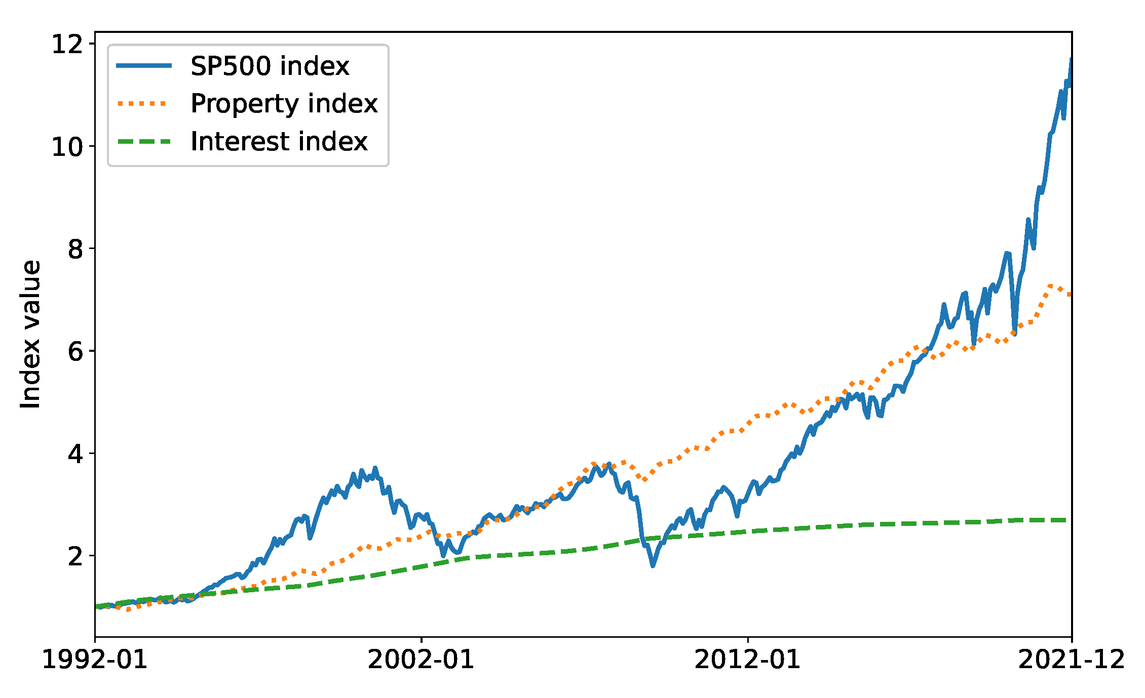
We continuously distribute funds into assets based on the indices of the S&P 500 [36], Norwegian property [37], and the Norwegian interest rate [38]. In addition, we invest in mortgages and luxury items. We show this data for a 30-year period in Figure 1.
We make a number of assumptions which limit the scope of the portfolio and simplify investment choices to make the characterization of agent behaviour and interpretation of investment strategies tractable.
Assumption 1.
Asset growth rates can be modelled by their respective asset indices, i.e., a stock portfolio may be modeled by a major stock index—e.g., the S&P 500, and an investment in property by its corresponding index.
The outright investment in indices such as S&P 500 is very common; it will return the growth rates according to these indices. This is a conservative assumption as stock portfolio optimization frequently outperforms indices, which may serve as a performance measure of the investment strategy [29].
To give personalised advice, we depart from the premise that there is a mere correlation between spending behaviour and happiness. We are expanding the notion of the causal relationship of spending patterns and customer satisfaction to chart an investment strategy and provide advice that is aligned with customer personality [18]. We enlisted a panel of experts from a major Norwegian bank to rate our asset classes according to a set of inherent properties: expected long term risk and returns, liquidity, minimum investment limits, and perceived novelty. We used the Sharpe ratio—the difference between the expected daily return and risk-free return divided by the standard deviation of daily returns—to quantify risk and historical data to gauge expected returns. These coefficients, the elements of a matrix P, are shown in Table 1.
The same panel of experts also assigned a matrix Q describing the likely associations between the prototypical personality traits and the asset classes, shown in Table 2. For instance, the conscientiousness trait might prefer assets classes with low expected risk, while the openness trait might prefer those which they perceive as novel.
From P and Q, we calculated a set of coefficients that describe the association that each personality trait might have with each of the asset classes. The resulting matrix of coefficients , normalized by column and scaled such that the values are in the range , are shown in Table 3.
We define a MDP for a multi-agent RL setting as follows:
- States A set of 13 continuous values representing the customer age (between 30 and 60 years and normalized to a range of ), six values for the asset class holdings and total portfolio value (scaled by ), and two market indicators for each of the three indices, i.e., their mean asset convergence divergence (MACD) (the difference between the 26-month and the 12-month exponential moving average of a trend) which predicts trend reversals and relative strength index ( where and are the average positive and negative changes to the index values respectively, for x periods) which corrects for potential false predictions by MACD. The time horizon is 30 years.
- Reward The changes in portfolio values between time steps.
- Actions The continuous distribution of funds across the five asset classes.
Assumption 2.
The initial values for a portfolio consist of a mortgage of NOK 2 million and a property valued at NOK 2 million. All other assets have zero initial value.
It is easy to adjust these initial portfolio assignments for different individuals.
Assumption 3.
We make consistent monthly investments of 10,000 Norwegian kroner (NOK).
This can be easily modified for individual customers’ contributions.
There is a priori no lower limit on the investment amounts:
Assumption 4.
Property investment does not require bulk payments, i.e., smaller investments can be made through property funds, trusts, or crowdfunding.
While investment in physical real estate normally requires larger deposits, we allow our agents to invest smaller amounts into the property market, i.e., a fraction of the monthly investment contribution specified in Assumption 3. This is not a strong assumption as it is possible to invest smaller amounts in property indices, trusts, funds, etc.
We assign interest rates for savings accounts at 5–10% below, and those of mortgage accounts at 5–10% over the interest index. Individuals younger than 35 years receive the more beneficial interest rate, as is common in Norwegian banks. Luxury items experience a depreciation of 20% per year; the depreciation of luxury items is highly variable and depends on the item, e.g., while artwork may appreciate, cars typically depreciate rapidly:
Assumption 5.
Luxury items depreciate at 20% per year.
Dividends are normally included in the calculation of indices and monthly transactions are relatively infrequent compared to high frequency trading:
Assumption 6.
Any additional income from investments—such as dividend payouts or rental income—as well as costs such as transaction costs and fund management costs are ignored.
3.2. Agents
We train five DDPG agents, one for each of the five personality traits. Using Equation (1) we regularise their objective functions with a prior derived from their respective personality traits in Table 3, e.g., the openness prior places the most weight on stocks and avoids mortgage repayments, property investment, and savings, while the conscientiousness prior places the most weight on mortgage repayments and avoids stocks and luxury expenditure. These priors, shown in Table 4, are probability distributions across the investment channels and therefore add up to one.
Our five agents have identical actor and critic networks, respectively. This is appropriate because they solve the same problem, but aim to find locally optimum policies in specific regions of the state-action space, as given by their respective regularisation priors. The 10 neural networks for the agents’ actors and critics each consist of two fully connected feed-forward layers with 2000 nodes in each layer. The actor networks each have a final soft-max activation layer while the critic networks have no final activations. The reason for the actors’ softmax activation is to ensure the values for the actions add up to one, while the critics need no activation as the rewards need not be scaled. We tuned the hyperparameters using a one-at-a-time parameter sweep resulting in learning rates of and for the actors and critics respectively, target network update parameters of , and regularisation coefficients of . Training batch sizes were 256 time steps and we sized the replay buffer to hold 2048 transitions. Each iteration collected 256 time steps and completed two training batches.
4. Results
Each of our investment agents learns an optimal investment strategy for their respective prototypical personality traits, for instance, openness. The final portfolio values after 334 months of investing according to these policies are shown in Table 5. Given the common total investment of 3.34 million NOK, the compound annual growth rate varies between 5.8% and 7.8% which is the maximum return possible if investing in stocks only.
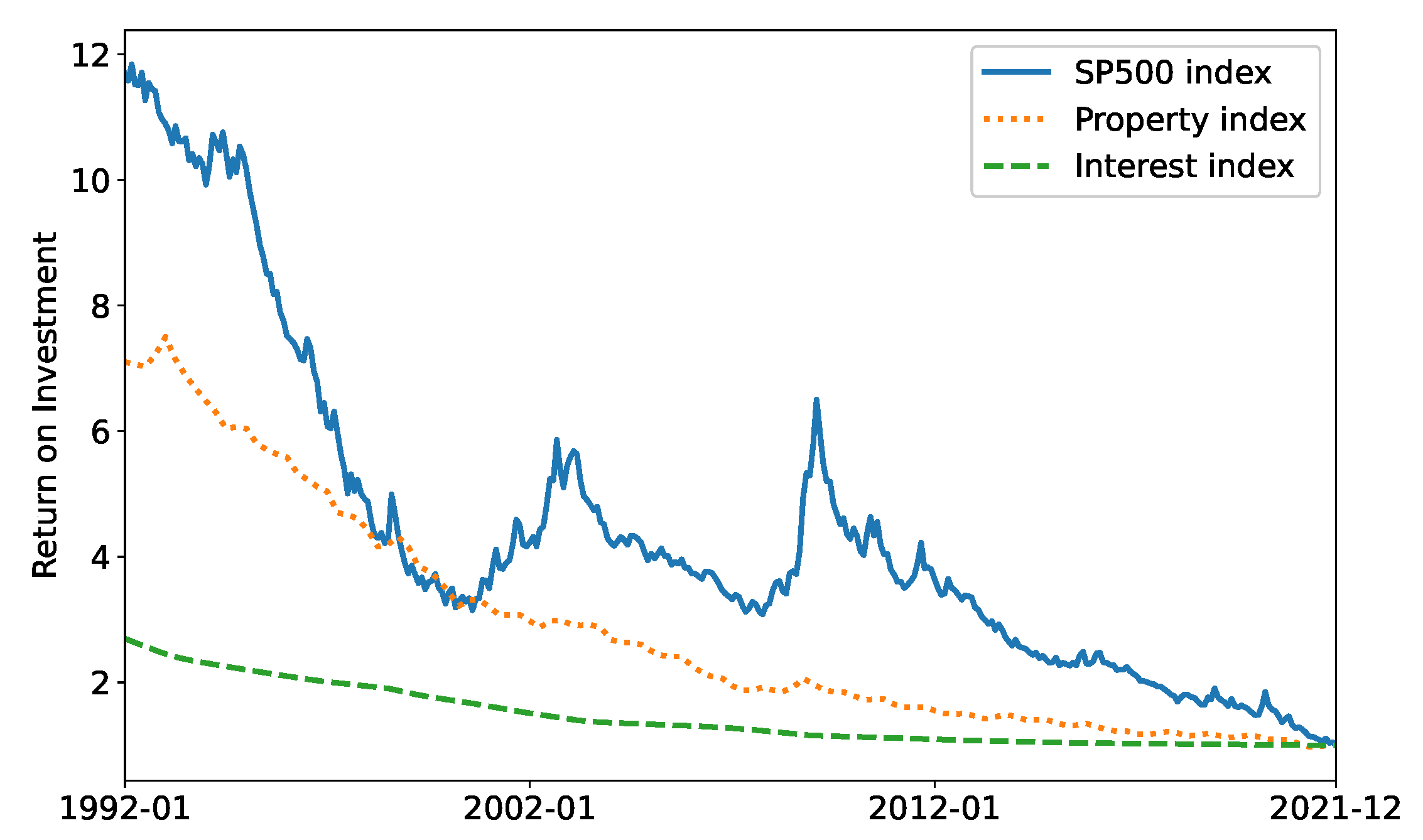
Note that these personalised policies did not achieve the same final portfolio value. In fact, the optimum policy in monetary terms in this case would have been to always buy stocks as shown in Figure 2; this is the default policy an agent will converge towards when personality traits are ignored.
However, we postulate that this is not the ideal personal financial advice to give to all individuals; some customers may be more averse to risk and will thus prefer to avoid volatility in their portfolio. Our personalized agent takes into account such preferences and, e.g., it recommends property investments rather than stock investments.
Thus far, our agents have each separately learned an optimal investment strategy for each prototypical personality trait. The aggregate policy is the weighted sum of these individually learned policies: a customer has a blend of personality traits which can be represented as a vector with five entries with values within the range . We calculate the inner product of the normalized personality vector and the prototypical policies to arrive at the aggregate investment policy. We show a representative aggregate investment policy for a customer with a random personality profile in Figure 3.
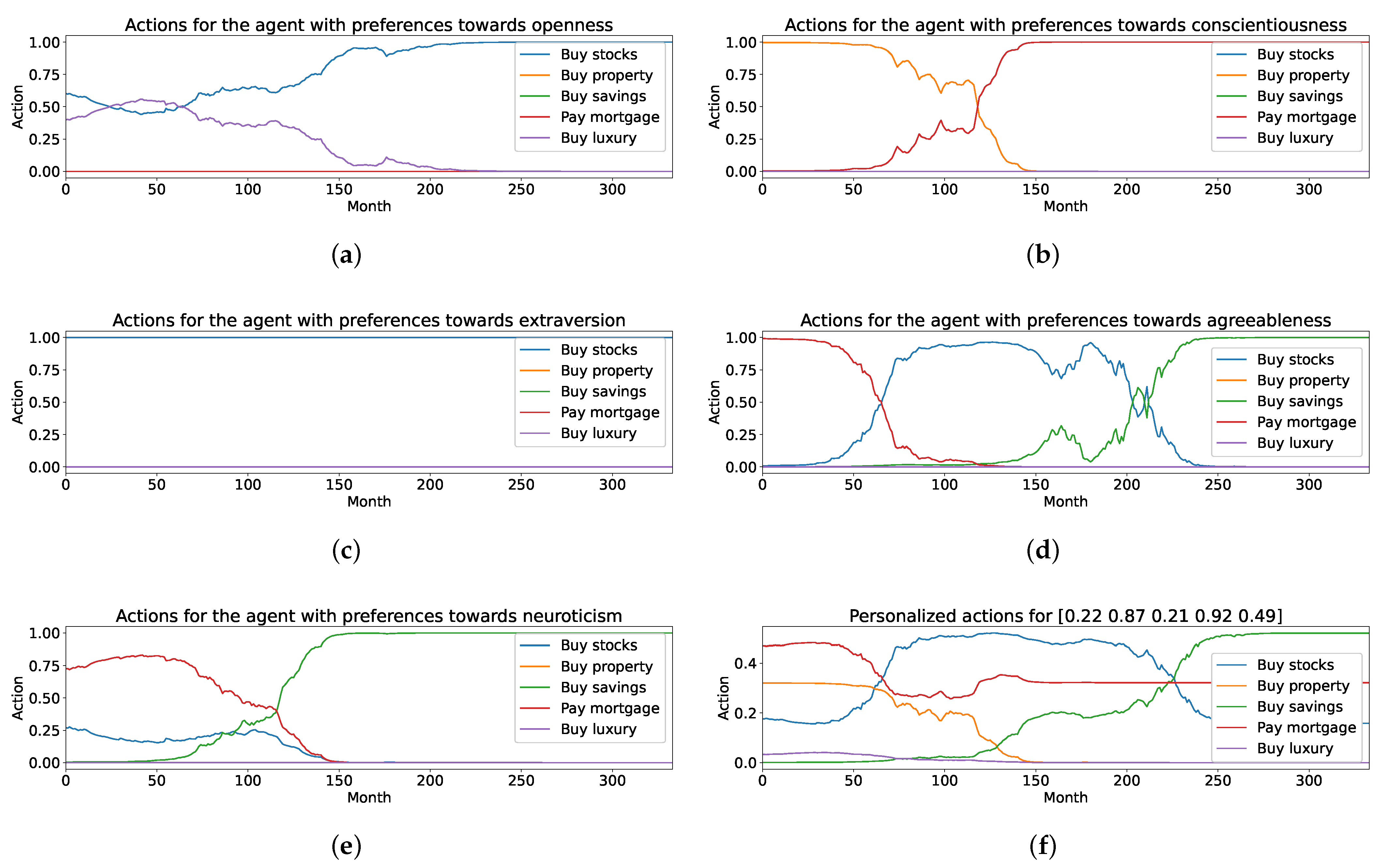
We observe that the openness agent is the only agent to recommend spending on luxury items; this is to be expected because its regularisation prior is the only one with a non-zero coefficient for luxury purchases. We also observe that the conscientiousness agent recommends investing in property in early stages, followed by rigorous loan repayments in the second half of the investment period. This suggests that our agent has learned the concept of compound growth and its utility for portfolio optimization. By contrast, the extraversion agent was steadfast in purchasing stocks only, which is consistent with its regularisation prior . Unlike the conscientiousness agent, the agreeableness and neuroticism agents consistently recommend investing in savings towards the end of the investment period. In the early stages of the investment period, the agreeableness and neuroticism agents utilize compound growth to increase the portfolio value; in the latter phases, their regimen changes and they prefer the safety of savings accounts. This is noteworthy because although risk is not explicitly part of either the reward or regularisation functions, it is consistent with traditional financial advice, which decreases the risk level with age. Repeated training produces consistent results. We intend to elucidate this observation in future work.
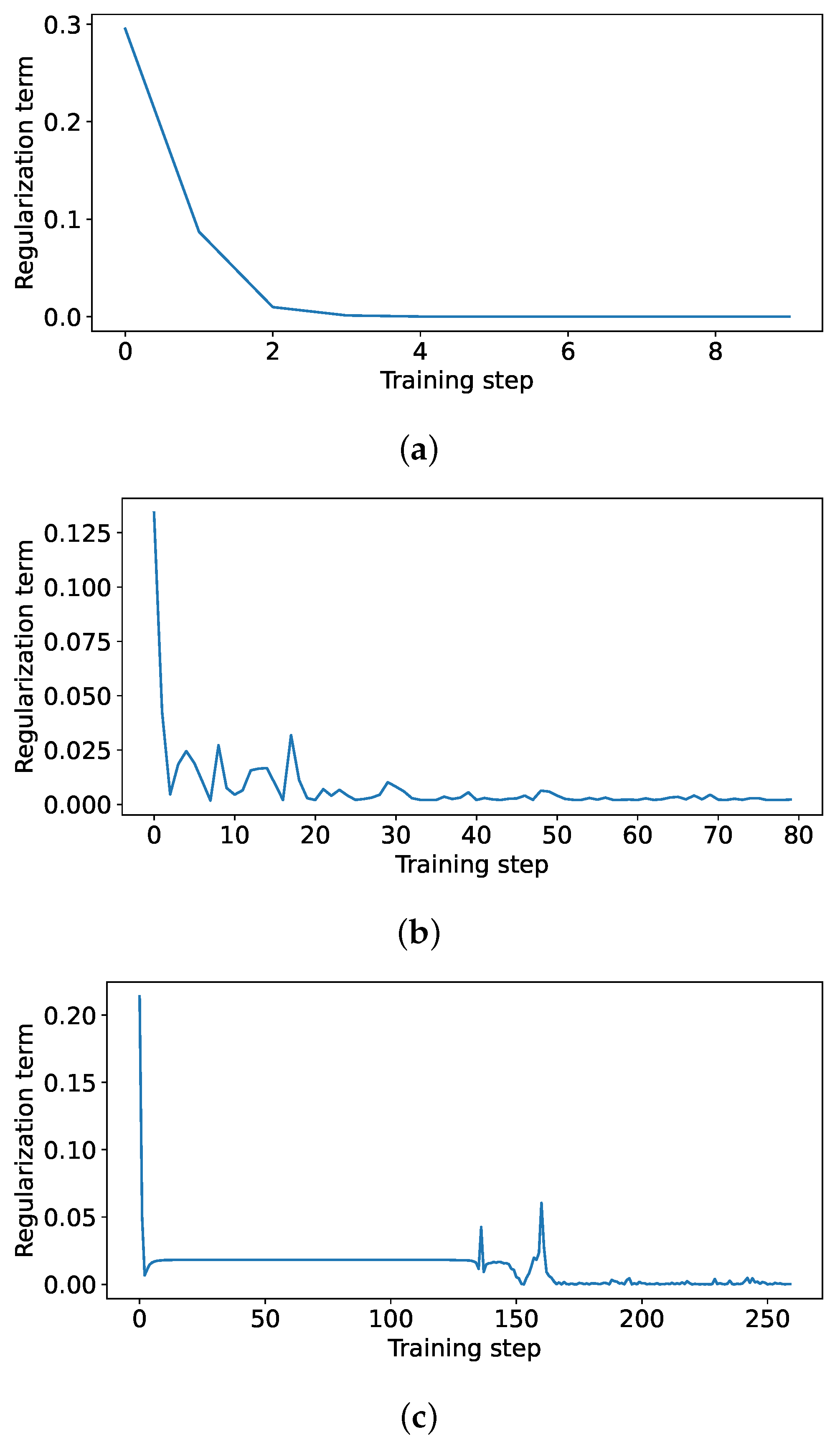
We observe that training converges quickly to the desired behaviour (see Figure 4); the contribution of the regularisation term decreases rapidly, which implies that the agent is learning the intended behaviour. We show the regularisation term for the extraversion agent where the regularisation prior matches the optimum monetary policy in Figure 4a. Further training causes no instability as is often observed in the DDPG algorithm [34]. We hypothesize that this may be due to the agent characteristics imposed by our regularisation whose effect may be similar to entropy regularisation [34].
The actions of any linear combination of these agents, i.e., any personal agent, are interpretable through the intrinsic characterizations, i.e., priors, of each of the regularized agents.
5. Conclusions and Directions for Future Work
We have presented a novel application of training RL agents to exhibit desired characteristics and behaviours in prosperity management. The method is based on the regularisation of the policy during training. Here, we use prototypical personality traits—openness, conscientiousness, agreeableness, extraversion, and neuroticism—to define a set of priors which express their affinity towards different assets and thus impose different investment strategies. This makes the agents’ behaviour explicit and thus offers an explanation for their recommendations. Our agents learn distinct optimal strategies for the continuous distribution of monthly investments across a portfolio of investment assets. We have shown that the agents learned to optimize total rewards while adhering to their distinct priors. This makes it possible to interpret the agents’ investment strategies.
Unlike traditional DDPG algorithms which may diverge with continuous training, our regularisation results in quick and robust convergence. This could become relevant if RL agents undergo continuous training to give personalized investment advice to customers. The justification of this observation will be subject to future research. Further, our regularisation method encourages exploration of a specific region in the action space, defined by the prior , which leads to a local optimum in near proximity of the prior. This is a specific case of the generalised entropy regularisation, which expedites convergence to the global optimum policy by encouraging exploration of the entire state-action space.
Our agents have learned the concept and utility of compound growth rates and risk avoidance, which form part of the interpretation of their investment strategies. These are solely based on the regularisation priors which express their personality traits; the reward function makes no reference to the personality traits. While the notion of compound growth may emerge from the reward function, we do not yet know whether the notion of risk avoidance is connected to the reward function or regularisation.
Here, we have chosen a linear combination of different, separately trained agents aligned with the prototypical personality traits to arrive at an aggregate investment advice. In the future, we will investigate whether the orchestration of these agents can be learned to approach the optimum monetary policy. This aggregation will need an explanation as well as interpretation to understand its impact on the investment strategy. The hierarchical orchestration of prototypical agents will be learned from real customers’ personality profiles. This will result in an explainable and interpretable personalized financial investment advisor.
Author Contributions
Conceptualization, C.M. and C.W.O.; methodology, C.M.; software, C.M.; validation, C.M.; formal analysis, C.M. and C.W.O.; investigation, C.M.; resources, C.M.; data curation, C.M.; writing—original draft preparation, C.M.; writing—review and editing, C.W.O. and C.M; visualization, C.M.; supervision, C.W.O.; project administration, C.M. and C.W.O.; funding acquisition, C.M. and C.W.O.; All authors have read and agreed to the published version of the manuscript.
Funding
This research was partially funded by The Norwegian Research Foundation, project number 311465.
Institutional Review Board Statement
Not applicable.
Informed Consent Statement
Not applicable.
Data Availability Statement
Not applicable.
Conflicts of Interest
The authors declare no conflict of interest. The funders had no role in the design of the study, in the collection, analyses, or interpretation of data, in the writing of the manuscript, or in the decision to publish the results.
References
- Stefanel, M.; Goyal, U. Artificial Intelligence & Financial Services: Cutting through the Noise; Technical Report; APIS Partners: London, UK, 2019. [Google Scholar]
- Jaiwant, S.V. Artificial Intelligence and Personalized Banking. In Handbook of Research on Innovative Management Using AI in Industry 5.0; Vikas, G., Goel, R., Eds.; IGI Global: Bengaluru, India, 2022; pp. 74–87. [Google Scholar]
- van der Burgt, J. General Principles for the Use of Artificial Intelligence in the Financial Sector; Technical Report; De Nederlandsche Bank: Amsterdam, The Netherlands, 2019. [Google Scholar]
- Oyebode, O.; Orji, R. A hybrid recommender system for product sales in a banking environment. J. Bank. Financ. Technol. 2020, 4, 15–25. [Google Scholar] [CrossRef]
- Bhatore, S.; Mohan, L.; Reddy, R. Machine learning techniques for credit risk evaluation: A systematic literature review. J. Bank. Financ. Technol. 2020, 4, 111–138. [Google Scholar] [CrossRef]
- Desai, D. Hyper-Personalization: An AI-Enabled Personalization for Customer-Centric Marketing. In Adoption and Implementation of AI in Customer Relationship Management; Singh, S., Ed.; IGI Global: Maharashtra, India, 2022; pp. 40–53. [Google Scholar]
- Jothimani, D.; Yadav, S. Stock trading decisions using ensemble-based forecasting models: A study of the Indian stock market. J. Bank. Financ. Technol. 2019, 3, 113–129. [Google Scholar] [CrossRef]
- Zhang, Q.; Yan, W.; Kankanhalli, M. Overview of currency recognition using deep learning. J. Bank. Financ. Technol. 2019, 3, 59–69. [Google Scholar] [CrossRef]
- Hsu, T.Y. Machine learning applied to stock index performance enhancement. J. Bank. Financ. Technol. 2021, 5, 21–33. [Google Scholar] [CrossRef]
- Kolm, P.; Ritter, G. Modern Perspectives on Reinforcement Learning in Finance. SSRN Electron. J. 2019, 1, 1–28. [Google Scholar] [CrossRef]
- Fischer, T.G. Reinforcement Learning in Financial Markets—A Survey; Technical Report; Friedrich-Alexander University Erlangen-Nuremberg, Institute for Economics: Erlangen, Germany, 2018. [Google Scholar]
- Barredo Arrieta, A.; Díaz-Rodríguez, N.; Del Ser, J.; Bennetot, A.; Tabik, S.; Barbado, A.; Garcia, S.; Gil-Lopez, S.; Molina, D.; Benjamins, R.; et al. Explainable Artificial Intelligence (XAI): Concepts, taxonomies, opportunities and challenges toward responsible AI. Inf. Fusion 2020, 58, 82–115. [Google Scholar] [CrossRef] [Green Version]
- Cao, L. AI in Finance: Challenges, Techniques and Opportunities. Bank. Insur. eJournal 2021, 14, 1–40. [Google Scholar] [CrossRef]
- Maree, C.; Modal, J.E.; Omlin, C.W. Towards Responsible AI for Financial Transactions. In Proceedings of the 2020 IEEE Symposium Series on Computational Intelligence (SSCI), Canberra, Australia, 1–4 December 2020; pp. 16–21. [Google Scholar]
- Maree, C.; Omlin, C. Reinforcement Learning Your Way: Agent Characterization through Policy Regularization. AI 2022, 3, 15. [Google Scholar] [CrossRef]
- Tasse, G.N.; James, S.; Rosman, B. A Boolean Task Algebra for Reinforcement Learning. In Proceedings of the Neural Information Processing Systems, Online, 6–12 December 2020; Volume 34, pp. 1–11. [Google Scholar]
- Gladstone, J.; Matz, S.; Lemaire, A. Can Psychological Traits Be Inferred From Spending? Evidence From Transaction Data. Psychol. Sci. 2019, 30, 1087–1096. [Google Scholar] [CrossRef] [PubMed] [Green Version]
- Matz, S.C.; Gladstone, J.J.; Stillwell, D. Money Buys Happiness When Spending Fits Our Personality. Psychol. Sci. 2016, 27, 715–725. [Google Scholar] [CrossRef] [PubMed]
- Maree, C.; Omlin, C.W. Clustering in Recurrent Neural Networks for Micro-Segmentation using Spending Personality. In Proceedings of the 2021 IEEE Symposium Series on Computational Intelligence (SSCI), Orlando, FL, USA, 5–7 December 2021; pp. 1–5. [Google Scholar]
- Maree, C.; Omlin, C.W. Understanding Spending Behavior: Recurrent Neural Network Explanation and Interpretation. In Proceedings of the IEEE Computational Intelligence for Financial Engineering and Economics, Helsinki, Finland, 4–5 May 2022; pp. 1–7, in print. [Google Scholar]
- Sutton, R.S.; Barto, A.G. Reinforcement Learning: An Introduction, 2nd ed.; The MIT Press: Cambridge, MA, USA, 2018. [Google Scholar]
- Bellman, R. A Markovian decision process. J. Math. Mech. 1957, 6, 679–684. [Google Scholar] [CrossRef]
- Lillicrap, T.P.; Hunt, J.J.; Pritzel, A.; Heess, N.; Erez, T.; Tassa, Y.; Silver, D.; Wierstra, D. Continuous control with deep reinforcement learning. arXiv 2019, arXiv:1509.02971. [Google Scholar]
- Bartram, S.M.; Branke, J.; Rossi, G.D.; Motahari, M. Machine Learning for Active Portfolio Management. J. Financ. Data Sci. 2021, 3, 9–30. [Google Scholar] [CrossRef]
- Jurczenko, E. Machine Learning for Asset Management: New Developments and Financial Applications; Wiley-ISTE: London, UK, 2020; pp. 1–460. [Google Scholar]
- Lim, Q.; Cao, Q.; Quek, C. Dynamic portfolio rebalancing through reinforcement learning. Neural Comput. Appl. 2021, 33, 1–15. [Google Scholar] [CrossRef]
- Pinelis, M.; Ruppert, D. Machine learning portfolio allocation. J. Financ. Data Sci. 2022, 8, 35–54. [Google Scholar] [CrossRef]
- Millea, A. Deep reinforcement learning for trading—A critical survey. Data 2021, 6, 119. [Google Scholar] [CrossRef]
- Maree, C.; Omlin, C.W. Balancing Profit, Risk, and Sustainability for Portfolio Management. In Proceedings of the IEEE Computational Intelligence for Financial Engineering and Economics, Helsinki, Finland, 4–5 May 2022; pp. 1–8, in print. [Google Scholar]
- Heuillet, A.; Couthouis, F.; Díaz-Rodríguez, N. Explainability in deep reinforcement learning. Knowl.-Based Syst. 2021, 214, 106685. [Google Scholar] [CrossRef]
- Wells, L.; Bednarz, T. Explainable AI and Reinforcement Learning: A Systematic Review of Current Approaches and Trends. Front. Artif. Intell. 2021, 4, 550030. [Google Scholar] [CrossRef] [PubMed]
- Gupta, S.; Singal, G.; Garg, D. Deep Reinforcement Learning Techniques in Diversified Domains: A Survey. Arch. Comput. Methods Eng. 2021, 28, 4715–4754. [Google Scholar] [CrossRef]
- Ziebart, B.D. Modeling Purposeful Adaptive Behavior with the Principle of Maximum Causal Entropy. Ph.D. Thesis, Machine Learning Department, Carnegie Mellon University, Pittsburgh, PA, USA, 2010. [Google Scholar]
- Haarnoja, T.; Tang, H.; Abbeel, P.; Levine, S. Reinforcement Learning with Deep Energy-Based Policies. In Proceedings of the International Conference on Machine Learning (ICML), Sydney, Australia, 6–11 August 2017. [Google Scholar]
- Knight Frank Company. Knight Frank Luxury Investment Index. 2022. Available online: https://www.knightfrank.com/wealthreport/luxury-investment-trends-predictions/ (accessed on 27 May 2022).
- Yahoo Finance. Historical Data for S&P500 Stock Index. 2022. Available online: https://finance.yahoo.com/quote/%5EGSPC/history?p=%5EGSPC, (accessed on 30 January 2022).
- Statistics Norway. Table 07221—Price Index for Existing Dwellings. 2022. Available online: https://www.ssb.no/en/statbank/table/07221/ (accessed on 30 January 2022).
- Norges Bank. Interest Rates. 2022. Available online: https://app.norges-bank.no/query/#/en/interest (accessed on 30 January 2022).
Figure 1.
Three asset value indices for a period of 30 years: The S&P 500 stock index, the Norwegian property index, and the Norwegian interest rate index. All indices are relative to their respective values on 1 January 1992. While the stock index performs the best overall, it has the highest volatility and therefore the highest risk. Conversely, the interest rate index has the lowest risk but also the lowest growth.

Figure 2.
The return on investment at every time step, calculated as the index value at the final time step divided by the index value at the current time step. It is clear that S&P 500 has the greatest return on investment at every time step, except for a brief period in ca. 2000 where it was marginally below the property index. Therefore, the optimum monetary policy is to always invest the maximum amount into stocks.

Figure 3.
Investment strategies for different prototypical personality traits: (a–e) show the fractions of monthly investments for different assets. They reveal the distinct investment strategies with changing asset preferences for the five prototypical personality traits. In (f) we illustrate the investment strategy for a fictitious customer with a random personality profile [openness, conscientiousness, agreeableness, extraversion, and neuroticism] = [0.22, 0.87, 0.21, 0.92, 0.49]. The customer invests in a mixture of assets throughout the investment period.

Figure 4.
The regularisation term L for three different runs. In (a) the regularisation prior of the extraverted agent coincides with the optimum monetary policy and the policy converges within 5 time steps. (b) shows a typical training run for the other agents which converges within 100–200 training steps. (c) shows a training run where the regularisation term appears to fall in local minimum for a time, but eventually finds the optimum after about 200 training steps.


Table 1.
A matrix P rating the performance of each asset class with respect to a set of desirable properties. Values are in range and represent a relative low to high score in each of the properties.
Table 1.
A matrix P rating the performance of each asset class with respect to a set of desirable properties. Values are in range and represent a relative low to high score in each of the properties.
| Asset Class Property | Savings | Property | Stocks | Luxury | Mortgage |
|---|---|---|---|---|---|
| High expected long term returns | 0.25 | 0.67 | 1.00 | 0.05 | 0.50 |
| Low expected long term risk | 1.00 | 0.32 | 0.10 | 0.05 | 1.00 |
| High asset liquidity | 1.00 | 0.25 | 0.80 | 0.10 | 0.05 |
| Low minimum investment | 0.80 | 0.25 | 1.00 | 0.50 | 1.00 |
| High perceived novelty | 0.10 | 0.25 | 0.75 | 1.00 | 0.10 |
Table 2.
A matrix Q describing the association between prototypical personality traits—openness (O), conscientiousness (C), extraversion (E), agreeableness (A), and neuroticism (N)—and a set of inherent properties of each asset class. Values are in and represent a highly negative, negative, neutral, positive and highly positive association, respectively.
| Asset Class Property | O | C | E | A | N |
|---|---|---|---|---|---|
| High expected long term returns | 1 | 1 | 2 | 1 | 1 |
| Low expected long term risk | −1 | 2 | −1 | 1 | 2 |
| High asset liquidity | 2 | −1 | 2 | 1 | 2 |
| Low minimum investment | 0 | −1 | 1 | 1 | 1 |
| High perceived novelty | 2 | 0 | 2 | 0 | −1 |
Table 3.
Coefficients relating asset risk, expected return, liquidity, capital requirement, and novelty to prototypical personality traits: openness (O), conscientiousness (C), extraversion (E), agreeableness (A), and neuroticism (N). The values are in the range .
Table 3.
Coefficients relating asset risk, expected return, liquidity, capital requirement, and novelty to prototypical personality traits: openness (O), conscientiousness (C), extraversion (E), agreeableness (A), and neuroticism (N). The values are in the range .
| Investment | O | C | E | A | N |
|---|---|---|---|---|---|
| Savings | −0.11 | 0.08 | −0.15 | 0.51 | 0.68 |
| Property | −0.15 | 0.32 | −0.22 | −0.36 | −0.24 |
| Stocks | 0.82 | −0.61 | 0.95 | 0.42 | 0.12 |
| Luxury | 0.16 | −0.51 | −0.07 | −0.80 | −0.81 |
| Mortgage | −0.72 | 0.72 | −0.52 | 0.23 | 0.25 |
Table 4.
Regularisation priors for each agent {openness (O), conscientiousness (C), extraversion (E), agreeableness (A), and neuroticism (N)}.
Table 4.
Regularisation priors for each agent {openness (O), conscientiousness (C), extraversion (E), agreeableness (A), and neuroticism (N)}.
| Investment | |||||
|---|---|---|---|---|---|
| Savings | 0.00 | 0.07 | 0.00 | 0.44 | 0.64 |
| Property | 0.00 | 0.28 | 0.00 | 0.00 | 0.00 |
| Stocks | 0.84 | 0.00 | 1.00 | 0.36 | 0.12 |
| Luxury | 0.16 | 0.00 | 0.00 | 0.00 | 0.00 |
| Mortgage | 0.00 | 0.65 | 0.00 | 0.02 | 0.24 |
Table 5.
Portfolio values of the five optimal policies for each of the prototypical personality traits.
Table 5.
Portfolio values of the five optimal policies for each of the prototypical personality traits.
| Policy | Final Portfolio Value (NOK 1M) |
|---|---|
| Openness | 22.4 |
| Conscientiousness | 18.8 |
| Extraversion * | 27.7 |
| Agreeableness | 20.5 |
| Neuroticism | 16.4 |
| Personal agent | 20.3 |
* This agent’s regularisation prior was coincidentally the same as the optimal monetary policy and it achieved the maximum possible final portfolio value.
Publisher’s Note: MDPI stays neutral with regard to jurisdictional claims in published maps and institutional affiliations. |
© 2022 by the authors. Licensee MDPI, Basel, Switzerland. This article is an open access article distributed under the terms and conditions of the Creative Commons Attribution (CC BY) license (https://creativecommons.org/licenses/by/4.0/).
Share and Cite
MDPI and ACS Style
Maree, C.; Omlin, C.W. Can Interpretable Reinforcement Learning Manage Prosperity Your Way? AI 2022, 3, 526-537. https://doi.org/10.3390/ai3020030
AMA Style
Maree C, Omlin CW. Can Interpretable Reinforcement Learning Manage Prosperity Your Way? AI. 2022; 3(2):526-537. https://doi.org/10.3390/ai3020030
Chicago/Turabian StyleMaree, Charl, and Christian W. Omlin. 2022. "Can Interpretable Reinforcement Learning Manage Prosperity Your Way?" AI 3, no. 2: 526-537. https://doi.org/10.3390/ai3020030