
Hydrogen-like Plasmas under Endohedral Cavity


Abstract
:1. Introduction
2. Theoretical Formalism
2.1. Oscillator Strength and Polarizability
2.2. Shannon Entropy
3. Result and Discussion
3.1. Critical Screening Constant in DHPWS and ECSCPWS
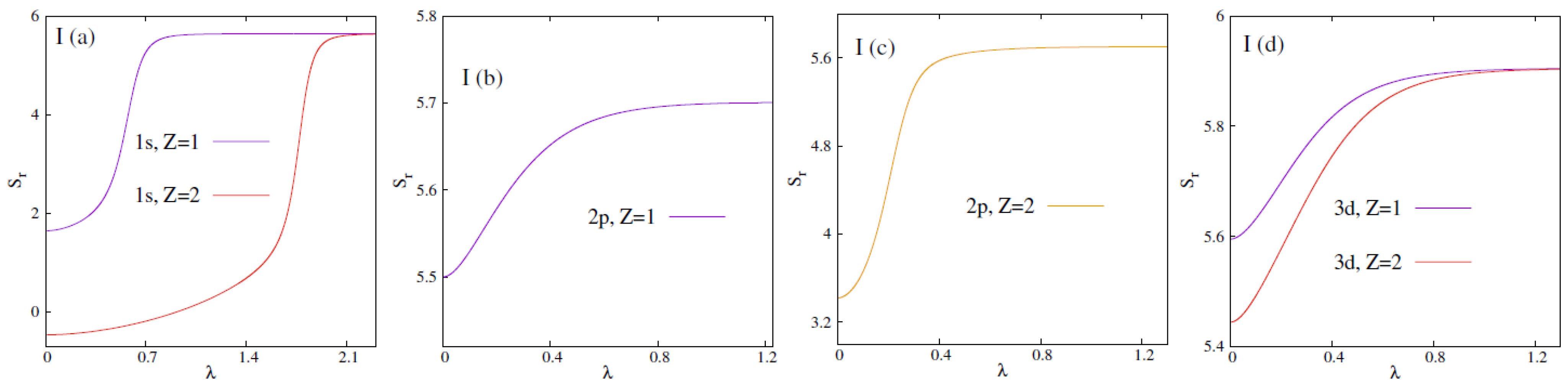
- At the onset, it should be mentioned that the qualitative behaviour of with in DHPWS and ECSCPWS are quite similar.
- Panels (I), (II) in Figure 1 show that there exists at least three bound states in either of the fullerene trapped plasmas. Because, in both cases, circular or node-less states with 0–2 are never going to be deleted. As a consequence, no abrupt jump in is observed. In these states increases with and finally converges to the respective limiting values.
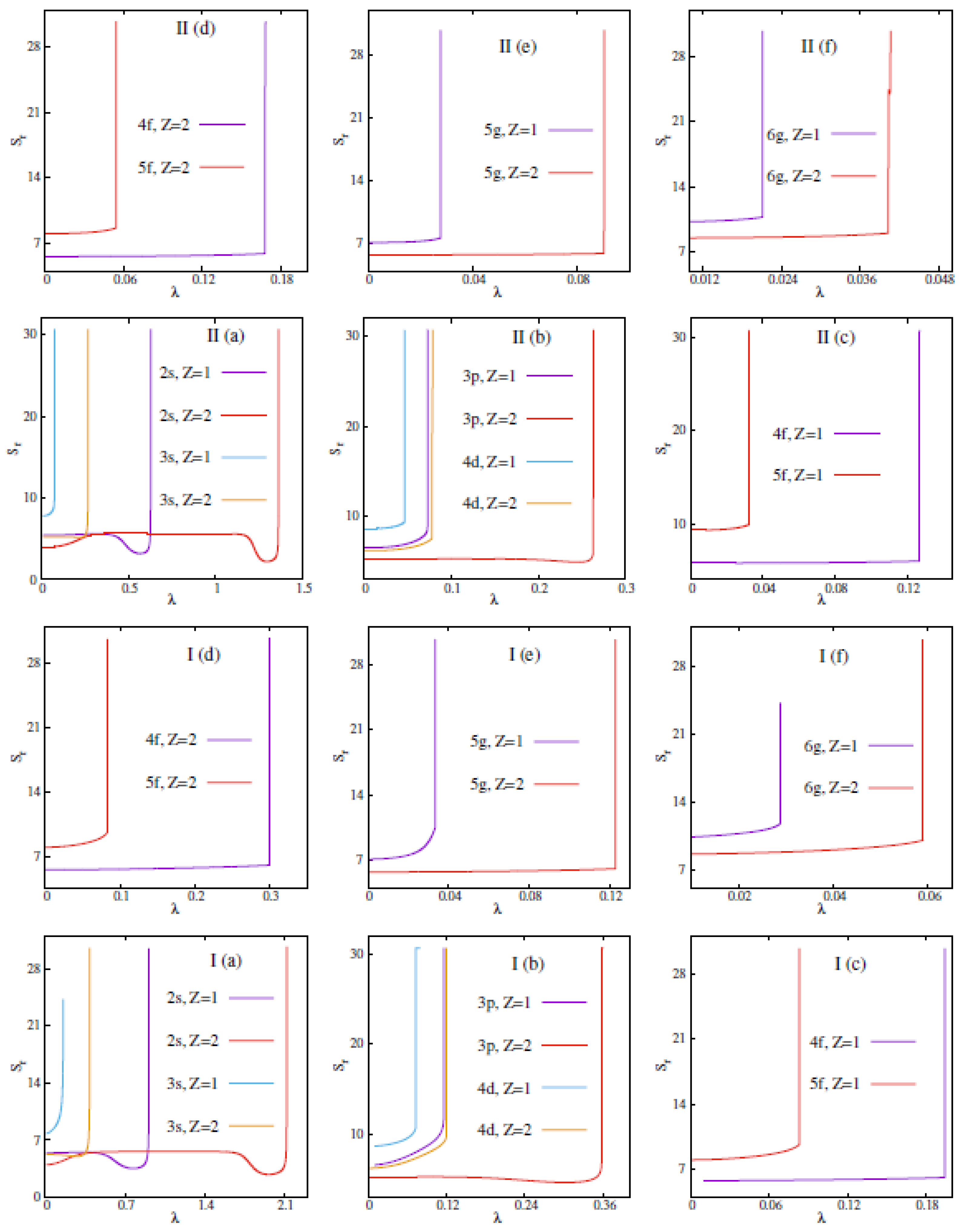
- Panels (I), (II) of Figure 2 suggest that, for a given state, there exists a characteristic at which the value jumps suddenly, signifying the phase transition. The position of these gets right shifted with a rise in Z. Here, a first order phase transition happens in both the plasmas involving states.
- These observations lead us to the conjecture that, in these two fullerene trapped plasmas, phase transition occurs for all states. However, for 0–2 states, a similar phenomenon occurs only when .
3.2. Dipole Oscillator Strength
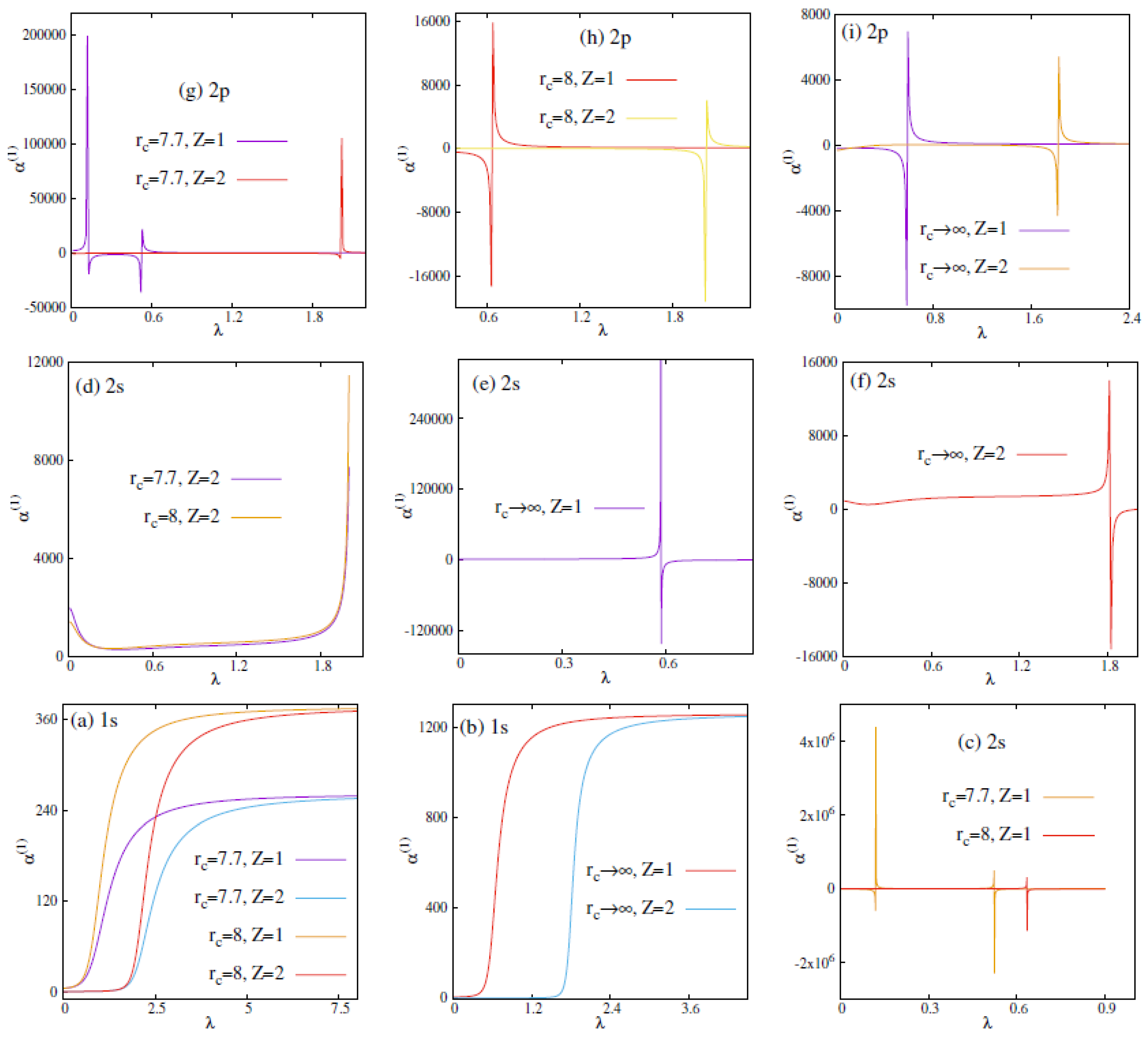
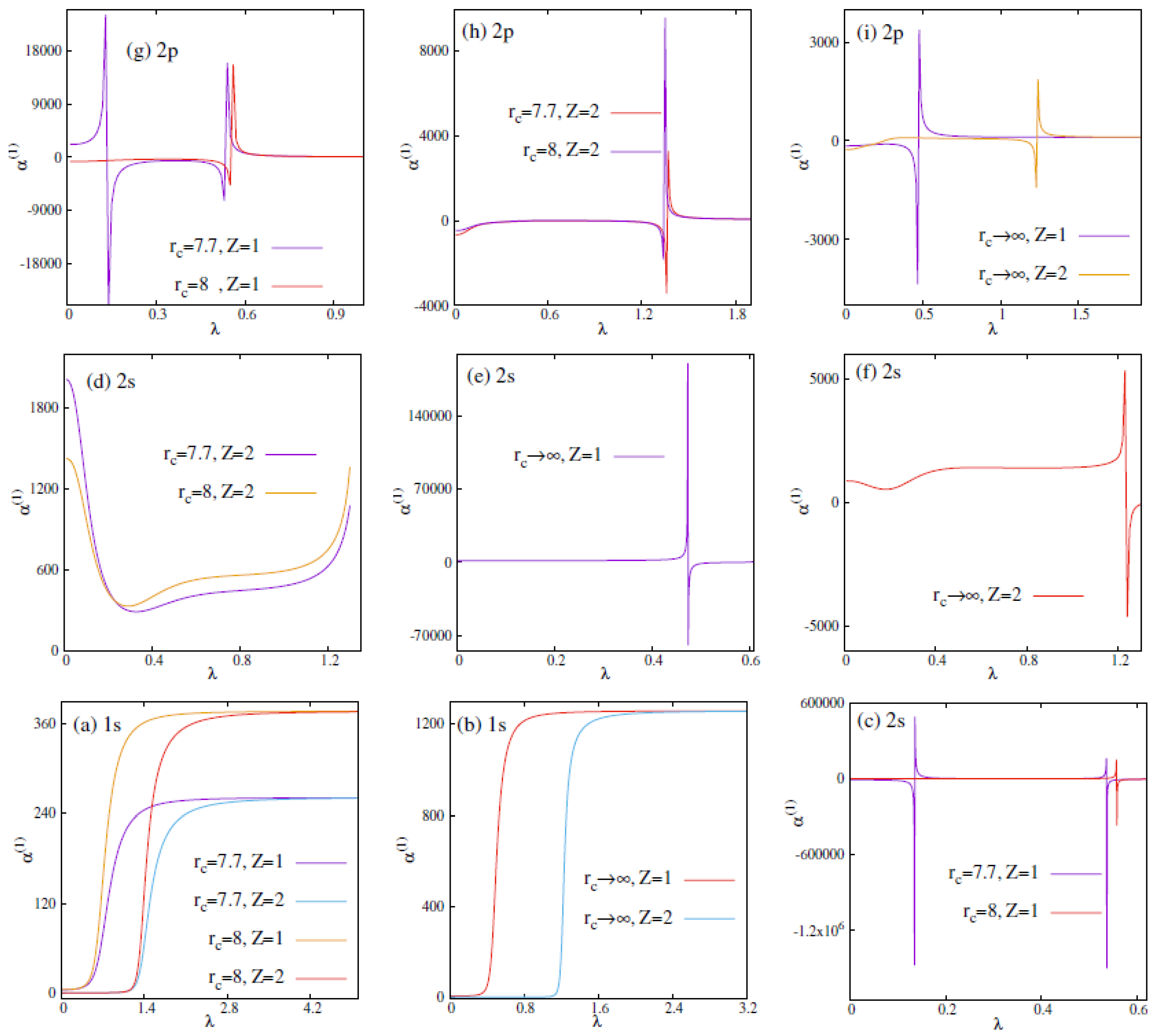
3.3. Polarizability
4. Conclusions
Author Contributions
Funding
Data Availability Statement
Acknowledgments
Conflicts of Interest
References
- Suryanarayana, D.; Weil, J.A. On the hyperfine splitting of the hydrogen atom in a spherical box. J. Chem. Phys. 1976, 64, 510. [Google Scholar] [CrossRef]
- Ley-Koo, E.; Rubinstein, S. The hydrogen atom inside boxes with paraboloidal surfaces. J. Chem. Phys. 1980, 73, 887. [Google Scholar] [CrossRef]
- Kilcoyne, A.L.D.; Aguilar, A.; Müller, A.; Schippers, S.; Cisneros, C.; Alna’Washi, G.; Aryal, N.B.; Baral, K.K.; Esteves, D.A.; Thomas, C.M.; et al. Confinement resonances in photoionization of Xe@C60+. Phys. Rev. Lett. 2010, 105, 213001. [Google Scholar] [CrossRef]
- Ndengué, S.A.; Motapon, O. Electric response of endohedrally confined hydrogen atoms. J. Phys. B At. Mol. Opt. Phys. 2008, 41, 045001. [Google Scholar] [CrossRef]
- Motapon, O.; Ndengué, S.A.; Sen, K.D. Static and dynamic dipole polarizabilities and electron density at origin: Ground and excited states of hydrogen atom confined in multiwalled fullerenes. Int. J. Quantum Chem. 2011, 111, 4425. [Google Scholar] [CrossRef]
- Benjamin, S.C.; Ardavan, A.; Briggs, G.A.D.; Britz, D.A.; Gunlycke, D.; Jefferson, J.; Jones, M.A.G.; Leigh, D.F.; Lovett, B.W.; Khlobystov, A.N.; et al. Towards a fullerene-based quantum computer. J. Phys. Condens. Matt. 2006, 18, S867. [Google Scholar] [CrossRef]
- Liu, Z.; Dong, B.W.; Meng, H.B.; Xu, M.X.; Wang, T.S.; Wang, B.W.; Wang, C.R.; Jiang, S.D.; Gao, S. Qubit crossover in the Endohedral fullerene Sc3C2@C80. Chem. Sci. 2018, 9, 457. [Google Scholar] [CrossRef]
- Yang, W.L.; Xu, Z.Y.; Wei, H.; Feng, M.; Suter, D. Quantum-information-processing architecture with endohedral fullerenes in a carbon nanotube. Phys. Rev. A 2010, 81, 032303. [Google Scholar] [CrossRef]
- Harneit, W. Fullerene-based electron-spin quantum computer. Phys. Rev. A 2002, 65, 032322. [Google Scholar] [CrossRef]
- Ross, R.B.; Cardona, C.M.; Guldi, D.M.; Sankaranarayanan, S.G.; Reese, M.O.; Kopidakis, N.; Peet, J.; Walker, B.; Bazan, G.C.; Van Keuren, E.; et al. Endohedral fullerenes for organic photovoltaic devices. Nat. Mater. 2009, 8, 208. [Google Scholar] [CrossRef]
- Ornes, S. Core Concept: Quantum dots. Proc. Natl. Acad. Sci. USA 2016, 113, 2796. [Google Scholar] [CrossRef] [PubMed]
- Nishikawa, K.; Wakatani, M. Plasma Physics: Basic Theory with Fusion Applications. In Plasma Physics: Basic Theory with Fusion Applications; Springer: Berlin/Heidelberg, Germany, 2010. [Google Scholar]
- Pupysheva, O.V.; Farajian, A.A.; Yakobson, B.I. Fullerene nanocage capacity for hydrogen storage. Nano Lett. 2008, 8, 767. [Google Scholar] [CrossRef] [PubMed]
- Shinohara, H. Endohedral metallofullerenes. Rep. Prog. Phys. 2000, 63, 843. [Google Scholar] [CrossRef]
- Kroto, H.W.; Heath, J.R.; O’Brien, S.C.; Curl, R.F.; Smalley, R.E. C60: Buckminsterfullerene. Nature 1985, 318, 162. [Google Scholar] [CrossRef]
- Amusia, M.Y.; Baltenkov, A.S.; Becker, U. Strong oscillations in the photoionization of 5s electrons in Xe@C60 endohedral atoms. Phys. Rev. A 2000, 62, 012701. [Google Scholar] [CrossRef]
- Patil, S.H.; Sen, K.D.; Varshni, Y.P. Alkali atoms confined to a sphere and to a fullerene cage. Can. J. Phys. 2005, 83, 919. [Google Scholar] [CrossRef]
- Kurotobi, K.; Murata, Y. A single molecule of water encapsulated in fullerene C60. Science 2011, 333, 613. [Google Scholar] [CrossRef]
- Amusia, M.Y.; Chernysheva, L.V.; Dolmatov, V.K. Confinement and correlation effects in the Xe@C60 generalized oscillator strengths. Phys. Rev. A 2011, 84, 063201. [Google Scholar] [CrossRef]
- Connerade, J.P.; Dolmatov, V.K.; Manson, S.T. A unique situation for an endohedral metallofullerene. J. Phys. B At. Mol. Opt. Phys. 1999, 32, L395. [Google Scholar] [CrossRef]
- Dolmatov, V.K.; Amusia, M.Y.; Chernysheva, L.V. Electron elastic scattering off A@C60: The role of atomic polarization under confinement. Phys. Rev. A 2015, 92, 042709. [Google Scholar] [CrossRef]
- Dolmatov, V.K.; Manson, S.T. Photoionization of atoms encapsulated in endohedral ions A@C60±z. Phys. Rev. A 2006, 73, 013201. [Google Scholar] [CrossRef]
- Moretto-Capelle, P.; Bordenave-Montesquieu, D.; Rentenier, A.; Bordenave-Montesquieu, A. Interaction of protons with the C60 molecule: Calculation of deposited energies and electronic stopping cross sections (v ≤ 5 au). J. Phys. B At. Mol. Opt. Phys. 2001, 34, L611. [Google Scholar] [CrossRef]
- Martínez-Flores, C. Shannon entropy and Fisher information for endohedral confined one-and two-electron atoms. Phys. Lett. A 2021, 386, 126988. [Google Scholar] [CrossRef]
- Martínez-Flores, C.; Cabrera-Trujillo, R. Derived properties from the dipole and generalized oscillator strength distributions of an endohedral confined hydrogen atom. J. Phys B At. Mol. Opt. Phys. 2018, 51, 055203. [Google Scholar] [CrossRef]
- Dolmatov, V.K.; Baltenkov, A.S.; Connerade, J.P.; Manson, S.T. Structure and photoionization of confined atoms. Radiat. Phys. Chem. 2004, 70, 417. [Google Scholar] [CrossRef]
- Nascimento, E.M.; Prudente, F.V.; Guimarães, M.N.; Maniero, A.M. A study of the electron structure of endohedrally confined atoms using a model potential. J. Phys. B At. Mol. Opt. Phys. 2010, 44, 015003. [Google Scholar] [CrossRef]
- Lin, C.Y.; Ho, Y.K. Photoionization of atoms encapsulated by cages using the power-exponential potential. J. Phys. B At. Mol. Opt. Phys. 2012, 45, 145001. [Google Scholar] [CrossRef]
- Bates, D.; Bederson, B. Advances in Atomic and Molecular Physics; Academic Press: Cambridge, MA, USA, 1989; Volume 25. [Google Scholar]
- Soylu, A. Plasma screening effects on the energies of hydrogen atom. Phys. Plasmas 2012, 19, 072701. [Google Scholar] [CrossRef]
- Bahar, M.K.; Soylu, A. The hydrogen atom in plasmas with an external electric field. Phys. Plasmas 2014, 21, 092703. [Google Scholar] [CrossRef]
- Paul, S.; Ho, Y.K. Hydrogen atoms in Debye plasma environments. Phys. Plasmas 2009, 16, 063302. [Google Scholar] [CrossRef]
- Bahar, M.K.; Soylu, A.; Poszwa, A. The hulthén potential model for hydrogen atoms in debye plasma. IEEE Trans. Plasma Sci. 2016, 44, 2297. [Google Scholar] [CrossRef]
- Jung, Y.D. Semiclassical transition probabilities for the electron-impact excitation of hydrogenic ions in dense plasmas. Phys. Plasmas 1995, 2, 332. [Google Scholar] [CrossRef]
- Jung, Y.D.; Yoon, J.S. Plasma-screening effects on semiclassical ionization probabilities for the electron-impact ionization of hydrogenic ions in dense plasmas. J. Phys. B At. Mol. Opt. Phys. 1996, 29, 3549. [Google Scholar] [CrossRef]
- Saha, B.; Mukherjee, P.K. Effect of Debye plasma on the structural properties of compressed positronium atom. Phys. Lett. A 2002, 302, 105. [Google Scholar] [CrossRef]
- Qi, Y.Y.; Wang, J.G.; Janev, R.K. Bound-bound transitions in hydrogenlike ions in Debye plasmas. Phys. Rev. A 2008, 78, 062511. [Google Scholar] [CrossRef]
- Qi, Y.Y.; Wang, J.G.; Janev, R.K. Static dipole polarizability of hydrogenlike ions in Debye plasmas. Phys. Rev. A 2009, 80, 032502. [Google Scholar] [CrossRef]
- Qi, Y.Y.; Wu, Y.; Wang, J.G.; Qu, Y.Z. The generalized oscillator strengths of hydrogenlike ions in Debye plasmas. Phys. Plasmas 2009, 16, 023502. [Google Scholar] [CrossRef]
- Das, M. Transition energies and polarizabilities of hydrogen like ions in plasma. Phys. Plasmas 2012, 19, 092707. [Google Scholar] [CrossRef]
- Kang, S.; Yang, Y.C.; He, J.; Xiong, F.Q.; Xu, N. The hydrogen atom confined in both Debye screening potential and impenetrable spherical box. Cent. Eur. J. Phys. 2013, 11, 584. [Google Scholar] [CrossRef]
- Gutierrez, F.A.; Diaz-Valdes, J. Effects of non-spherical screening for inelastic electron-ion scattering. J. Phys. B At. Mol. Opt. Phys. 1994, 27, 593. [Google Scholar] [CrossRef]
- Yoon, J.S.; Jung, Y.D. Spherical versus nonspherical plasma-screening effects on semiclassical electron–ion collisional excitations in weakly coupled plasmas. Phys. Plasmas 1996, 3, 3291. [Google Scholar] [CrossRef]
- Paul, S.; Ho, Y.K. Three-photon transitions in the hydrogen atom immersed in Debye plasmas. Phys. Rev. A 2009, 79, 032714. [Google Scholar] [CrossRef]
- Paul, S.; Ho, Y.K. Two-photon transitions in hydrogen atoms embedded in weakly coupled plasmas. Phys. Plasmas 2008, 15, 073301. [Google Scholar] [CrossRef]
- Zan, L.R.; Jiao, L.G.; Ma, J.; Ho, Y.K. Information-theoretic measures of hydrogen-like ions in weakly coupled Debye plasmas. Phys. Plasmas 2017, 24, 122101. [Google Scholar] [CrossRef]
- Bassi, M.; Baluja, K.L. Polarizability of screened Coulomb potential. Indian J. Phys. 2012, 86, 961. [Google Scholar] [CrossRef]
- Lin, C.Y.; Ho, Y.K. Effects of screened Coulomb (Yukawa) and exponential-cosine-screened Coulomb potentials on photoionization of H and He+. Eur. Phys. J. D 2010, 57, 21. [Google Scholar] [CrossRef]
- Lam, C.S.; Varshni, Y.P. Bound eigenstates of the exponential cosine screened coulomb potential. Phys. Rev. A 1972, 6, 1391. [Google Scholar] [CrossRef]
- Lai, C.S. Energies of the exponential cosine screened Coulomb potential. Phys. Rev. A 1982, 26, 2245. [Google Scholar] [CrossRef]
- Dutt, R.; Mukherji, U.; Varshni, Y.P. Energy levels and oscillator strengths for the exponential-cosine screened Coulomb potential in the shifted large-dimension expansion theory. J. Phy. B At. Mol. Phys. 1986, 19, 3411. [Google Scholar] [CrossRef]
- Bayrak, O.; Boztosun, I. Application of the asymptotic iteration method to the exponential cosine screened Coulomb potential. Int. J. Quantum Chem. 2007, 107, 1040. [Google Scholar] [CrossRef]
- Singh, D.; Varshni, Y.P. Accurate eigenvalues and oscillator strengths for the exponential-cosine screened Coulomb potential. Phys. Rev. A 1983, 28, 2606. [Google Scholar] [CrossRef]
- Paul, S.; Ho, Y.K. Solution of the generalized exponential cosine screened Coulomb potential. Comput. Phys. Commun. 2011, 182, 130. [Google Scholar] [CrossRef]
- Nasser, I.; Abdelmonem, M.S.; Abdel-Hady, A. J-Matrix approach for the exponential-cosine-screened Coulomb potential. Phys. Script. 2011, 84, 045001. [Google Scholar] [CrossRef]
- Qi, Y.Y.; Wang, J.G.; Janev, R.K. Bound-bound transitions in hydrogen-like ions in dense quantum plasmas. Phys. Plasmas 2016, 23, 073302. [Google Scholar] [CrossRef]
- Roy, A.K. Studies on some exponential-screened coulomb potentials. Int. J. Quantum Chem. 2013, 113, 1503. [Google Scholar] [CrossRef]
- Lai, H.F.; Lin, Y.C.; Lin, C.Y.; Ho, Y.K. Bound-state energies, oscillator strengths, and multipole polarizabilities for the hydrogen atom with exponential-cosine screened coulomb potentials. Chin. J. Phys. 2013, 51, 73. [Google Scholar]
- Kuganathan, N.; Arya, A.K.; Rushton, M.J.D.; Grimes, R.W. Trapping of volatile fission products by C60. Carbon 2018, 132, 477. [Google Scholar] [CrossRef]
- Brocławik, E.; Eilmes, A. Density functional study of endohedral complexes M@C60 (M = Li, Na, K, Be, Mg, Ca, La, B, Al): Electronic properties, ionization potentials, and electron affinities. J. Chem. Phys. 1998, 108, 3498. [Google Scholar] [CrossRef]
- Kikuchi, K.; Kobayashi, K.; Sueki, K.; Suzuki, S.; Nakahara, H.; Achiba, Y.; Tomura, K.; Katada, M. Encapsulation of radioactive 159Gd and 161Tb atoms in fullerene cages. J. Am. Chem. Soc. 1994, 116, 9775. [Google Scholar] [CrossRef]
- Martínez-Flores, C.; Cabrera-Trujillo, R. Dipole and generalized oscillator strength derived electronic properties of an endohedral hydrogen atom embedded in a Debye-Hückel plasma. Matter Radiat. Extreme 2018, 3, 227. [Google Scholar] [CrossRef]
- Mukherjee, N.; Patra, C.N.; Roy, A.K. Confined hydrogenlike ions in plasma environments. Phys. Rev. A 2021, 104, 012803. [Google Scholar] [CrossRef]
- Roy, A.K. Studies on bound-state spectra of Manning–Rosen potential. Mod. Phys. Lett. A 2014, 29, 1450042. [Google Scholar] [CrossRef]
- Roy, A.K. Confinement in 3D polynomial oscillators through a generalized pseudospectral method. Mod. Phys. Lett. A 2014, 29, 1450104. [Google Scholar] [CrossRef]
- Roy, A.K. Ro-vibrational spectroscopy of molecules represented by a Tietz–Hua oscillator potential. J. Math. Chem. 2014, 52, 1405. [Google Scholar] [CrossRef]
- Mukherjee, N.; Roy, A.K. Quantum mechanical virial-like theorem for confined quantum systems. Phys. Rev. A 2019, 99, 022123. [Google Scholar] [CrossRef]
- Mukherjee, N.; Roy, A.K. Analysis of Compton profile through information theory in H-like atoms inside impenetrable sphere. J. Phys. B At. Mol. Opt. Phys. 2020, 53, 235002. [Google Scholar] [CrossRef]
- Zhu, L.; He, Y.Y.; Jiao, L.G.; Wang, Y.C.; Ho, Y.K. Revisiting the generalized pseudospectral method: Radial expectation values, fine structure, and hyperfine splitting of confined atom. Int. J. Quantum Chem. 2020, 120, e26245. [Google Scholar] [CrossRef]
- Ghoshal, A.; Ho, Y.K. Photodetachment of H− in dense quantum plasmas. Phys. Rev. E 2010, 81, 016403. [Google Scholar] [CrossRef]
- Xu, Y.B.; Tan, M.Q.; Becker, U. Oscillations in the photoionization cross section of C60. Phys. Rev. Lett. 1996, 76, 3538. [Google Scholar] [CrossRef]
- Dolmatov, V.K.; King, J.L.; Oglesby, J.C. Diffuse versus square-well confining potentials in modelling A@C60 atoms. J. Phys. B At. Mol. Opt. Phys. 2012, 45, 105102. [Google Scholar] [CrossRef]
- Connerade, J.P.; Dolmatov, V.K.; Lakshmi, P.A.; Manson, S.T. Electron structure of endohedrally confined atoms: Atomic hydrogen in an attractive shell. J. Phys. B At. Mol. Opt. Phys. 1999, 32, L239. [Google Scholar] [CrossRef]
- Hasoğlu, M.F.; Zhou, H.L.; Manson, S.T. Correlation study of endohedrally confined alkaline-earth-metal atoms A@C60. Phys. Rev. A 2016, 93, 022512. [Google Scholar] [CrossRef]
- Puska, M.J.; Nieminen, R.M. Photoabsorption of atoms inside C60. Phys. Rev. A 1993, 47, 1181. [Google Scholar] [CrossRef] [PubMed]
- Madjet, M.E.; Chakraborty, H.S.; Rost, J.M.; Manson, S.T. Photoionization of C60: A model study. J. Phys B At. Mol. Opt. Phys. 2008, 41, 105101. [Google Scholar] [CrossRef]
- Yan, Z.C.; Babb, J.F.; Dalgarno, A.; Drake, G.W.F. Variational calculations of dispersion coefficients for interactions among H, He, and Li atoms. Phys. Rev. A 1996, 54, 2824. [Google Scholar] [CrossRef]
- Luyckx, R.; Coulon, P.H.; Lekkerkerker, H.N.W. Dispersion interaction between helium atoms. Chem. Phys. Lett. 1977, 48, 187. [Google Scholar] [CrossRef]
- Bartolotti, L.J. Oscillator strength sum rule and the hydrodynamic analogy to quantum mechanics. Chem. Phys. Lett. 1979, 60, 507. [Google Scholar] [CrossRef]
- Mukherjee, N.; Roy, A.K. Information-entropic measures in free and confined hydrogen atom. Int. J. Quantum Chem. 2018, 118, e25596. [Google Scholar] [CrossRef]
- Estanón, C.R.; Aquino, N.; Puertas-Centeno, D.; Dehesa, J.S. Two-dimensional confined hydrogen: An entropy and complexity approach. Int. J. Quantum Chem. 2020, 120, e26192. [Google Scholar] [CrossRef]
- Jiao, L.G.; Zan, L.R.; Zhang, Y.Z.; Ho, Y.K. Benchmark values of Shannon entropy for spherically confined hydrogen atom. Int. J. Quantum Chem. 2017, 117, e25375. [Google Scholar] [CrossRef]
- Salazar, S.J.C.; Laguna, H.G.; Dahiya, B.; Prasad, V.; Sagar, R.P. Shannon information entropy sum of the confined hydrogenic atom under the influence of an electric field. Eur. Phys. J. D 2021, 75, 127. [Google Scholar] [CrossRef]


| DHPWS | ECSCPWS | ||||||
|---|---|---|---|---|---|---|---|
| State | State | ||||||
| 1 | − | − | 1 | − | − | ||
| 2 | − | − | 2 | − | − | ||
| 1 | −0.000000254 | 1 | 0.6287 | −0.000000038 | |||
| 2 | 2.1247 | −0.000000197 | 2 | 1.3618 | −0.000000165 | ||
| 1 | −0.000000439 | 1 | 0.0762 | −0.000000130 | |||
| 2 | 0.3900 | −0.000000055 | 2 | 0.2688 | −0.000000238 | ||
| 1 | − | − | 1 | − | − | ||
| 2 | − | − | 2 | − | − | ||
| 1 | −0.000000096 | 1 | 0.0730 | −0.000001331 | |||
| 2 | 0.3575 | −0.000011586 | 2 | 0.2633 | −0.000053585 | ||
| 1 | − | − | 1 | − | − | ||
| 2 | − | − | 2 | − | − | ||
| 1 | 0.0732 | −0.000000291 | 1 | 0.0466 | −0.000003059 | ||
| 2 | 0.1197 | −0.000005269 | 2 | 0.0782 | −0.000064445 | ||
| 1 | 0.1947 | −0.000000856 | 1 | 0.1267 | −0.000007139 | ||
| 2 | 0.2994 | −0.000023163 | 2 | 0.1681 | −0.000018290 | ||
| 1 | 0.0472 | −0.000016099 | 1 | 0.0323 | −0.000001631 | ||
| 2 | 0.0831 | −0.000007057 | 2 | 0.0540 | −0.000038551 | ||
| 1 | 0.0333 | −0.000000778 | 1 | 0.0278 | −0.000006697 | ||
| 2 | 0.1231 | −0.000005413 | 2 | 0.0903 | −0.000078050 | ||
| 1 | 0.0288 | −0.000005039 | 1 | 0.0210 | −0.000001928 | ||
| 2 | 0.0588 | −0.000040341 | 2 | 0.0403 | −0.000068680 | ||
| Transition | DHPWS | ECSCPWS | |||||||
|---|---|---|---|---|---|---|---|---|---|
| 1s→2p | 0.01 | 0.472909 | 0.405489 | 0.393008 | 0.399455 | 0.473031 | 0.405670 | 0.393153 | 0.399658 |
| 0.1 | 0.463893 | 0.389264 | 0.382538 | 0.380980 | 0.466412 | 0.399214 | 0.385322 | 0.392167 | |
| 0.5 | 0.506522 | 0.146559 | 0.445168 | 0.104184 | 0.506896 | 0.062774 | 0.475507 | 0.036498 | |
| 1.0 | 0.859970 | 0.072607 | 0.881023 | 0.047763 | 0.941505 | 0.069773 | 0.911234 | 0.051167 | |
| 2.5 | 0.937700 | 0.910538 | 0.902761 | 0.915478 | 0.918853 | 0.924631 | 0.884901 | 0.889980 | |
| 2p→1s | 0.01 | −0.157636 | −0.135163 | −0.131002 | −0.133151 | −0.157677 | −0.135223 | −0.131051 | −0.133219 |
| 0.1 | −0.154631 | −0.129754 | −0.127512 | −0.126993 | −0.155470 | −0.133071 | −0.128440 | −0.130722 | |
| 0.5 | −0.168840 | −0.048853 | −0.148389 | −0.034728 | −0.168965 | −0.020924 | −0.158502 | −0.012166 | |
| 1.0 | −0.286656 | −0.024202 | −0.293674 | −0.015921 | −0.313835 | −0.023257 | −0.303744 | −0.017055 | |
| 2.5 | −0.312566 | −0.303512 | −0.300920 | −0.305159 | −0.306284 | −0.308210 | −0.294967 | −0.296660 | |
| 2p→3d | 0.01 | 1.088693 | 0.800227 | 1.082666 | 0.732754 | 1.088689 | 0.800197 | 1.082677 | 0.732695 |
| 0.1 | 1.088778 | 0.806429 | 1.081425 | 0.743057 | 1.088627 | 0.798441 | 1.081926 | 0.731705 | |
| 0.5 | 1.071869 | 1.055338 | 1.054450 | 1.060247 | 1.055825 | 1.067797 | 1.036342 | 1.050053 | |
| 1.0 | 1.052710 | 1.063993 | 1.034850 | 1.045177 | 1.039857 | 1.036862 | 1.023702 | 1.020954 | |
| 2.5 | 1.043849 | 1.044600 | 1.027258 | 1.027832 | 1.042933 | 1.042720 | 1.026567 | 1.026410 | |
| 3d→2p | 0.01 | −0.653216 | −0.480136 | −0.649599 | −0.439652 | −0.653213 | −0.480118 | −0.649606 | −0.439617 |
| 0.1 | −0.653267 | −0.483857 | −0.648855 | −0.445834 | −0.653176 | −0.479064 | −0.649156 | −0.439023 | |
| 0.5 | −0.643121 | −0.633202 | −0.632670 | −0.636148 | −0.633495 | −0.640678 | −0.621805 | −0.630032 | |
| 1.0 | −0.631626 | −0.638396 | −0.620910 | −0.627106 | −0.623914 | −0.622117 | −0.614221 | −0.612572 | |
| 2.5 | −0.626309 | −0.626760 | −0.616355 | −0.616699 | −0.625760 | −0.625632 | −0.615940 | −0.615846 | |
| 3d→4f | 0.01 | 1.361677 | 1.378364 | 1.350361 | 1.374690 | 1.361703 | 1.378352 | 1.350391 | 1.374693 |
| 0.1 | 1.359552 | 1.378857 | 1.347923 | 1.373824 | 1.360468 | 1.378527 | 1.348914 | 1.374145 | |
| 0.5 | 1.342821 | 1.355667 | 1.330534 | 1.342513 | 1.333760 | 1.336163 | 1.321648 | 1.322866 | |
| 1.0 | 1.334518 | 1.337464 | 1.322958 | 1.325371 | 1.329986 | 1.328230 | 1.319261 | 1.317836 | |
| 2.5 | 1.331894 | 1.331979 | 1.320806 | 1.320868 | 1.331802 | 1.331794 | 1.320741 | 1.320736 | |
| Transition | DHPWS | ECSCPWS | ||||||
|---|---|---|---|---|---|---|---|---|
| 1s→2p | 0.01 | 0.149983 | 0.01 | 0.377669 | 0.01 | 0.150086 | 0.01 | 0.378002 |
| 0.1 | 0.143844 | 0.1 | 0.345192 | 0.1 | 0.143408 | 0.1 | 0.363852 | |
| 0.5 | 0.405345 | 0.5 | 0.014097 | 0.5 | 0.795304 | 0.5 | 0.003368 | |
| 1.0 | 0.853185 | 1.0 | 0.008094 | 1.0 | 0.815081 | 1.0 | 0.015977 | |
| 2.5 | 0.813876 | 2.5 | 0.829531 | 2.5 | 0.809188 | 2.5 | 0.810333 | |
| 2p→1s | 0.01 | −0.049994 | 0.01 | −0.125889 | 0.01 | −0.050028 | 0.01 | −0.126000 |
| 0.1 | −0.047948 | 0.1 | −0.115064 | 0.1 | −0.047802 | 0.1 | −0.121284 | |
| 0.5 | −0.135115 | 0.5 | −0.004699 | 0.5 | −0.265101 | 0.5 | −0.001122 | |
| 1.0 | −0.284395 | 1.0 | −0.002698 | 1.0 | −0.271693 | 1.0 | −0.005325 | |
| 2.5 | −0.271292 | 2.5 | −0.276510 | 2.5 | −0.269729 | 2.5 | −0.270111 | |
| 2p→3d | 0.01 | 1.062893 | 0.01 | 0.511654 | 0.01 | 1.062940 | 0.01 | 0.511243 |
| 0.1 | 1.059233 | 0.1 | 0.563033 | 0.1 | 1.061126 | 0.1 | 0.525528 | |
| 0.5 | 1.039334 | 0.5 | 1.058267 | 0.5 | 1.033436 | 0.5 | 1.037782 | |
| 1.0 | 1.032612 | 1.0 | 1.035607 | 1.0 | 1.029282 | 1.0 | 1.028293 | |
| 2.5 | 1.030470 | 2.5 | 1.030594 | 2.5 | 1.030324 | 2.5 | 1.030294 | |
| 3d→2p | 0.01 | −0.637736 | 0.01 | −0.306992 | 0.01 | −0.637764 | 0.01 | −0.306745 |
| 0.1 | −0.635539 | 0.1 | −0.337820 | 0.1 | −0.636675 | 0.1 | −0.315316 | |
| 0.5 | −0.623600 | 0.5 | −0.634960 | 0.5 | −0.620061 | 0.5 | −0.622669 | |
| 1.0 | −0.619567 | 1.0 | −0.621364 | 1.0 | −0.617569 | 1.0 | −0.616975 | |
| 2.5 | −0.618282 | 2.5 | −0.618356 | 2.5 | −0.618194 | 2.5 | −0.618176 | |
| 3d→4f | 0.01 | 1.358996 | 0.01 | 1.377113 | 0.01 | 1.358989 | 0.01 | 1.377140 |
| 0.1 | 1.358827 | 0.1 | 1.374730 | 0.1 | 1.358891 | 0.1 | 1.376182 | |
| 0.176 | 1.352618 | 0.15 | 1.372349 | 0.12602 | 1.354588 | 0.157 | 1.372370 | |
| 0.1931 | 1.347244 | 0.255 | 1.364948 | 0.12638 | 1.354413 | 0.16724 | 1.369061 | |
| 0.19462 | 1.346487 | 0.29949 | 1.354689 | 0.12671 | 1.354225 | 0.16812 | 1.368517 | |
| State | DHPWS | ECSCPWS | |||||||
|---|---|---|---|---|---|---|---|---|---|
| Z = 1 | Z = 2 | Z = 1 | Z = 2 | Z = 1 | Z = 2 | Z = 1 | Z = 2 | ||
| 1s | 0.01 | 4.657831 | 0.28128622 | 4.746857 | 0.2812862 | 4.6554220 | 0.2812521 | 4.7442022 | 0.2812521 |
| 0.1 | 4.881931 | 0.28451405 | 4.994924 | 0.2845141 | 4.7251882 | 0.2817758 | 4.8232375 | 0.2817759 | |
| 0.5 | 12.2287 | 0.35794112 | 14.6516 | 0.3579433 | 17.04331 | 0.3321934 | 24.00875 | 0.3321963 | |
| 1.0 | 78.7749 | 0.69849914 | 140.048 | 0.6990358 | 202.0018 | 1.1380112 | 320.2554 | 1.1591198 | |
| 2.5 | 230.696 | 128.19895 | 345.626 | 226.2246 | 259.3304 | 251.0688 | 375.0790 | 367.0643 | |
| 3.0 | 240.868 | 187.73712 | 356.253 | 299.8536 | 260.2497 | 256.3160 | 375.9265 | 372.1057 | |
| 2s | 0.01 | −6323.6041 | 1974.66567 | 2449.20791 | 1407.62883 | −6259.74897 | 2014.6251 | 2455.03251 | 1427.48523 |
| 0.1 | −25,299.096 | 762.542243 | 2096.11187 | 671.915445 | −12,087.9810 | 1214.6507 | 2197.55093 | 975.180845 | |
| 0.5 | 18,546.933 | 297.184946 | 2569.87340 | 369.786944 | 4830.94856 | 368.81438 | 2570.99350 | 481.397967 | |
| 1.0 | −252.97113 | 421.447127 | −232.042760 | 527.012512 | −26.4762447 | 481.38339 | −9.29681306 | 592.581494 | |
| 2.5 | 9.5211800 | −128.377389 | 18.4890829 | −86.8752095 | 29.6816393 | 21.677927 | 36.7365367 | 29.6077279 | |
| 3.0 | 16.629850 | −29.6973425 | 24.7934626 | −13.1804006 | 30.8831256 | 27.068895 | 37.7878081 | 34.3689306 | |
| 2p | 0.01 | 2191.410 | −643.03504 | −702.8776 | −452.1602 | 2170.076 | −656.3755 | −704.8910 | −458.8075 |
| 0.1 | 8520.618 | −237.05905 | −579.3616 | −204.1988 | 4114.992 | −388.9010 | −615.7853 | −306.8603 | |
| 0.5 | −6061.053 | −24.508518 | −694.8934 | −13.59247 | −1473.332 | −1.579597 | −678.1659 | 9.116706 | |
| 1.0 | 204.2574 | −8.8332529 | 219.5863 | −0.670906 | 100.0618 | −6.121894 | 97.77017 | −1.240847 | |
| 2.5 | 79.78501 | 152.51948 | 81.67296 | 148.6793 | 67.74707 | 71.51052 | 70.12450 | 73.50398 | |
| 3.0 | 75.37053 | 102.96430 | 77.42353 | 103.0182 | 67.26899 | 69.03491 | 69.71802 | 71.31396 | |
| State | DHPWS | ECSCPWS | ||||||
|---|---|---|---|---|---|---|---|---|
| 1s | 0.01 | 5.041120 | 0.01 | 0.2812863 | 0.01 | 5.0373245 | 0.01 | 0.2812522 |
| 0.1 | 5.405572 | 0.1 | 0.2845141 | 0.1 | 5.1638458 | 0.1 | 0.2817760 | |
| 0.5 | 71.4353 | 0.5 | 0.3579454 | 0.5 | 553.3792 | 0.5 | 0.3321994 | |
| 1.0 | 1076.49 | 1.0 | 0.7000504 | 1.0 | 1241.072 | 1.0 | 1.2523499 | |
| 2.5 | 1242.28 | 2.5 | 1183.049 | 2.5 | 1257.825 | 2.5 | 1254.207 | |
| 3.0 | 1247.93 | 3.0 | 1220.684 | 3.0 | 1258.140 | 3.0 | 1256.377 | |
| 2s | 0.01 | 1480.865 | 0.01 | 871.382822 | 0.01 | 1480.571 | 0.01 | 877.9676 |
| 0.1 | 1507.894 | 0.1 | 578.058339 | 0.1 | 1497.317 | 0.05 | 845.6145 | |
| 0.3 | 1720.036 | 0.5 | 1060.98797 | 0.2 | 1587.219 | 0.09 | 738.4854 | |
| 0.5 | 2721.953 | 1.0 | 1338.07651 | 0.3 | 1771.873 | 0.3 | 940.9011 | |
| 0.7 | −326.1830 | 1.5 | 1503.41076 | 0.5 | −1276.650 | 0.7 | 1404.159 | |
| 0.9 | 23008.31 | 2.0 | −23.222516 | 0.6 | 259.9035 | 1.3 | −65.30549 | |
| 2p | 0.01 | −150.7481 | 0.01 | −262.0658419 | 0.01 | −150.9188 | 0.01 | −264.3678 |
| 0.1 | −139.2984 | 0.1 | −152.6892619 | 0.1 | −140.9449 | 0.1 | −201.3010 | |
| 0.5 | −443.5363 | 0.5 | 69.93496507 | 0.5 | 786.5248 | 0.5 | 87.43362 | |
| 1.0 | 168.1365 | 1.0 | 64.90555224 | 1.0 | 114.3632 | 1.0 | 55.87104 | |
| 2.5 | 111.5520 | 2.5 | 133.2633406 | 2.5 | 106.2537 | 2.5 | 107.5945 | |
| 3.0 | 109.6328 | 3.0 | 119.4094711 | 3.0 | 106.1153 | 3.0 | 106.7672 | |
Disclaimer/Publisher’s Note: The statements, opinions and data contained in all publications are solely those of the individual author(s) and contributor(s) and not of MDPI and/or the editor(s). MDPI and/or the editor(s) disclaim responsibility for any injury to people or property resulting from any ideas, methods, instructions or products referred to in the content. |
© 2023 by the authors. Licensee MDPI, Basel, Switzerland. This article is an open access article distributed under the terms and conditions of the Creative Commons Attribution (CC BY) license (https://creativecommons.org/licenses/by/4.0/).
Share and Cite
Chowdhury, S.; Mukherjee, N.; Roy, A.K. Hydrogen-like Plasmas under Endohedral Cavity. Quantum Rep. 2023, 5, 459-474. https://doi.org/10.3390/quantum5020030
Chowdhury S, Mukherjee N, Roy AK. Hydrogen-like Plasmas under Endohedral Cavity. Quantum Reports. 2023; 5(2):459-474. https://doi.org/10.3390/quantum5020030
Chicago/Turabian StyleChowdhury, Saptarshi, Neetik Mukherjee, and Amlan K. Roy. 2023. "Hydrogen-like Plasmas under Endohedral Cavity" Quantum Reports 5, no. 2: 459-474. https://doi.org/10.3390/quantum5020030